摘要:稍不均匀电场间隙的起始击穿路径问题对于气体放电触发以及电极表面削蚀有重要意义. 为研究低气压击穿工况中起始路径的位置规律, 本文建立了一种基于蒙特卡罗碰撞模型与电子运动轨迹假设相结合的路径判断模型(determination of the critical path 模型, DCP模型), 并以2种电极装置的击穿试验来验证DCP模型的正确性. 通过负电极表面的痕迹捕捉和击穿电压的测量可以分别验证DCP模型对起始击穿路径和击穿电压的计算能力. 根据试验结果, 起始击穿路径在不同压强或流率下会发生转移, 且转移趋势与计算结果相符; 同时, DCP模型对击穿电压的计算误差不超过7.9%, 可初步验证DCP模型的计算精度. 在此基础上, 利用DCP模型对其他4种典型的电极装置进行数值计算, 发现全部击穿案例都存在一些共性: 随着间隙压强或流率的升高, 最小电压区域((pd) min过渡区)的起始路径转移频繁, 并伴随击穿电压上下波动, 近似持平, 且起始路径几乎都服从较长路径向较短路径的转移规律. 最后, 通过DCP模型的数值分析, 揭示了上述起始路径相关规律的内在机理.
关键词: 稍不均匀电场间隙/
起始击穿路径/
路径转移/
数值模拟

English Abstract

全文HTML

--> --> -->

本文研究所提到的稍不均匀电场的间隙是指电场不均匀系数f在2.0—4.0 (f为电场中最大场强与平均场强的比值)的电极间隙. 在低压气体击穿的研究中, f在2.0—4.0的电极是较为常见的工程研究对象, 主要涉及真空环境下的气体放电触发以及电极表面的削蚀等问题. 近年来, 尤其在空间电推进领域, 推进系统的点火性能设计常涉及到非匀强电场的低压击穿问题, 多次气体放电工况中的电极表面打火点是目前比较受关注的研究方向.
根据经典帕邢定律^[1], 在无限大的两平行电极间, 临界击穿电压(能够引发击穿的电压下限, 下文均简称击穿电压)与电极间距d和间隙压强p的乘积有关, 其击穿电压曲线呈现为“U”型. 在此类工况中, 电极间的电场分布、压强分布都均匀, 间隙距离处处相等, 那么在击穿间隙的所有区域都会发生电子雪崩, 这种击穿过程可认为是一种全通道的放电过程. 然而, 在非匀强电场电极的工况中, 击穿放电并非全通道放电. Golden等^[2,3]首先发现非匀强电场电极下的击穿电压与汤森放电模型的预估值不一致, 认为汤森电离系数在描述非匀强电场的电离次数时, 在不同间隙位置的描述方式会存在差异, 所以对汤森第一电离系数做出了修正, 得到了与试验较吻合的结果, 这是首次发现非匀强电场工况与全通道放电工况的机制不同. 接着, Osmokrovic等^[4,5] 针对几种典型复杂电极进行了击穿电压的测量试验, 通过分析试验结果, 发现复杂电极间的击穿总会存在一个“临界区域”, 该区域会首先触发击穿, 接着击穿过程将快速蔓延至整个放电通道, 但在他的研究中仅说明这种“临界区域”会随着压强、电极结构的不同而改变, 没有揭示如何确定这种“临界区域”的具体位置, 并且相关的物理机制尚不清晰. 然而, 对于非匀强电场的电极来说, 获得“临界区域”的位置对于预估击穿电压以及研究电极点火的主要削蚀点均有着重要意义. 鉴于试验方法具有一定局限性, 因此, 本文将采用数值与试验结合的方法来对“临界区域”(本文称之为起始击穿路径)进行研究.
到目前为止, 关于低气压放电路径的数值研究鲜有报道, 所以本文将从高气压放电路径的研究来获得一些借鉴与启发. 由于高气压下的放电路径在大量统计数据中既具备一定的自相似性, 又会在流注传导时表现出一定的随机性. 于是, 根据这种客观物理规律, Niemeyer 等^[6]建立了经典的流注分形模型, 主要实现流注顶端的电场强度能否维持放电持续的判断以及放电发展方向的随机判断. 接着, 如果考虑放电初始电场与放电中的电势降, 则需要修改电场强度的求解模型^[7]. 在此基础上, Niemeyer^[8]又提出先导的随机漫步模型, 通过在拉普拉斯背景电场中建立线性曲线坐标系来实现多条潜在先导路径的划分, 并计算了当地先导的扩散度, 进而求解了当地先导的扩散概率方程以实现放电路径的模拟, 所得计算结果的图像就像先导在无数阶梯中进行随机漫步一样. 但在实际情况中, 放电通道的电介质不都是均匀分布的, 因而还需要考虑将电导率、介电常数进行空间函数化处理, 以修正空间各位置的放电扩散概率^[9]. 随后的研究, 主要表现为对扩散概率、分形维度等经验参数的修正^[10-12].
实际上, 高气压的流注模型与低气压的电子雪崩模型有本质区别, 分形理论并不能适用于低气压的放电路径模拟. 但是, 通过对流注分形模型的认知, 可以确定低气压放电路径模拟需要2个关键条件: 第一, 模型应具备对放电维持的判断; 第二, 模型应具备对潜在放电路径的划分, 并且这种划分要符合客观规律(高气压的放电路径具有随机性, 故流注模型利用概率判断的扩散分形方法就非常符合客观规律). 因此, 本文在建立低气压放电的起始路径模型时将充分考虑这2个条件.
首先, 根据汤森放电理论, 电子雪崩放电过程的维持必须要有电离碰撞作为先决条件^[13], 由此, 应引入模拟电离碰撞等相关的碰撞概率模型, 在以往的等离子体放电研究中, 蒙特卡罗模型是比较成熟的碰撞概率判断模型, 该模型曾应用于强电场间隙的逃逸电子流模拟^[14,15]、小间隙的击穿放电模拟^[16], 获得了计算结果与试验结果较高的吻合度. 其次, 低气压下的背景气体数密度较低, 这使得电子与背景气体发生弹性碰撞散射的概率较低. 同时, 电子运动受电场力约束较显著, 在击穿过程中即使发生散射也会再漂移到附近区域的电场线中, 从统计学角度来看, 这类似于一群电子沿着相邻几条电场线迁移. 因此, 本文采用“电子沿电场线”的运动假设, 认为潜在的击穿起始路径由若干条电场线组成, 且该假设在Macheret和Shneider^[17]的“非散射传导”(forward-back)模型中也有体现. 结合上述2个条件, 我们建立一种基于电场线路径假设、蒙特卡罗碰撞模型的起始路径判断模型(determination of the critical path, DCP模型). 接着, 为验证DCP模型的计算精度, 开展2种电极结构的击穿放电试验, 以说明DCP模型的有效性. 在此基础上, 将DCP模型应用于其他4种有代表性结构的电极计算中, 获得稍不均匀电场下低气压击穿起始路径的位置规律和相关物理内涵.

为实现稍不均匀电场间的起始路径预估, 我们建立起DCP模型. 此模型的建立思想为: 在电极间隙中寻找一条最可能发生击穿的起始路径, 若该路径刚好可以触发局部击穿过程, 则整个间隙将完成临界击穿.
DCP模型的整体计算流程如下:
Step.1 基于“电场线为电子运动轨迹”假设, 在电极间划分若干条候选击穿路径(可能成为起始击穿路径的路径);
Step.2 设定电极间的电压差(电极电压U₀), 并将划分好的候选击穿路径以等电势线正交分割开来, 以路径线和等势线的交点为计算节点;
Step.3 在负电极表面的每一个计算节点设定相等数量(n₀)的初始电子, 这些初始电子在电极电压的作用下会沿着各自的候选路径向正电极运动, 沿程计算电子动能变化、各类碰撞概率;
Step.4 统计每一条候选路径所发生的总电离次数以及所产生的正离子数量, 并计算这些正离子撞击负电极表面所产生的二次电子数量(n_γ);
Step.5 筛选所有候选路径中n_γ最多的一条记为起始击穿路径, 并判断这条起始路径的n_{γ, max}与n₀之间的关系. 若n_{γ, max}明显低于n₀, 则无法实现击穿, 适当升高电极电压(更新Step.2中的U₀, 继续迭代计算); 若n_{γ, max}明显高于n₀, 则触发“过量击穿”, 适当降低电极电压(更新Step.2中的U₀, 继续迭代计算); 若满足n_{γ, max}接近n₀, 则刚好实现临界击穿(计算收敛).
具体物理模型细节将于下文详细介绍.
2

-->

2.1.计算节点划分

首先, 进行间隙中候选击穿路径的划分. 假定在负电极表面存在一些均匀分布的初始电子, 以这些电子来代表间隙中由宇宙射线等外界因素所触发的原始电子. 这些负电极表面的电子将会沿着各自的候选路径, 在电极电压(U₀)的作用下运动到正电极表面. 这里, 由于低气压汤森放电中的空间电荷效应不显著, 忽略空间净电荷分布对电场的影响. 那么, 如果假设电子的运动路径为电场线, 则这些负电极表面均布的电子会通过均匀划分的候选路径向正电极运动(图1).
图 1 典型非平行电极间的计算节点划分示意图
Figure1. Schematic diagram of the mesh grid generation in nonparallel two-electrode gap

接着, 以若干电位等势线来分割候选路径, 使得所分割的微元路径上的电势降都相等. 于是, 整个间隙中由等势线和候选路径形成的交点, 就是计算节点.
2 -->

2.2.电子动能及碰撞概率

假设每一条候选路径从负电极表面都会触发n₀个初始电子向正电极运动. 这些电子会在电极电压(U₀)的作用下增加动能, 并触发与背景中性气体的碰撞过程.
根据2.1小节的阐述, 电子在任意候选路径上运动时, 每经过一个微元路径, 将会降低相同的电势能($\Delta U \cdot {e}$), 而动能将增加$\Delta U \cdot {e}$(e为元电荷, $1.6 \times {10^{ - 19}}{\rm{ C}}$). 那么, 当电子具有一定动能时, 必将触发与中性气体的碰撞.
根据蒙特卡罗碰撞(Monte-Carlo collisions, MCC)模型, 一个电子在中性气体中, 在极短时间$\Delta t$内的碰撞概率为

$P = 1 - {{\rm{e}}^{ - {f_{\rm{en}}}\Delta t}},$

其中, ${f_{\rm{en}}}$为电子与原子间的碰撞频率, $\Delta t$为电子经过一个微元路径所用的时间(s).

${f_{{\rm{en}}}} = {N_{\rm{n}}} \cdot {v_{{\rm{en}}}} \cdot {\sigma _T}({E_{k, e}}),$

其中, ${N_{\rm{n}}}$为中性气体的数密度(m^–3), 在计算中通常会出现2种情形:
第一种, 间隙压强均匀分布, ${N_{\rm{n}}}$为常数, 这种情况可以由式(3)计算:

${N_{\rm{n}}}{\rm{ = }}\frac{{{P_{{\rm{gap}}}}}}{{{k_{\rm{B}}}T}},$

其中, ${P_{{\rm{gap}}}}$为间隙压强(Pa), ${k_{\rm{B}}}$为玻尔兹曼常数(${k_{\rm{B}}} = 1.38 \times {10^{ - 23}}{\rm{ J/K}}$), $T$为背景气体温度(K).
第二种, 如果间隙压强分布不均匀(通常由气体流动产生), 则需要通过求解数密度分布场来获得某一网格节点下的数密度分布数据, 但是, 求解数密度的网格节点与DCP模型的计算节点划分一般不同, 所以还需要利用插值(通常采用权重法)来获得DCP计算节点的${N_{\rm{n}}}$. 图2给出了典型空心阴极的气体流动间隙中的${N_{\rm{n}}}$计算方法.
图 2 间隙压强不均布时的${N_{\rm{n}}}$计算方法
Figure2. Computational method of the ${N_{\rm{n}}}$ in the gap of non-uniform pressure distribution

其次, (2)式中的${v_{\rm{en}}}$为电子与原子的相对速度, 由于背景气体运动速度远低于电子, ${v_{\rm{en}}}$可认为是电子本身的运动速度${v_e}$.

${v_e} = \sqrt {2{\rm{e}}{E_{k,e}}/{m_e}},$

其中, ${E_{k,e}}$为电子动能(eV), ${m_e}$为电子质量(kg).
接着, (2)式中的${\sigma _T}({E_{k,e}})$为电子与中性原子的总碰撞截面(m²), 由于后文的试验与计算工质主要采用氙(Xe), 因此, 这里以Xe为例来进行介绍.
根据表1, 总碰撞截面${\sigma _T}\left({E_{k,e}}\right)$可以由3种碰撞截面之和来计算:

碰撞类型	碰撞截面公式/m2
弹性碰撞	$1.699 \times {10^{ - 19}}$	${E_{k,e}} \leqslant 0.159\; {\rm{ eV}}$
	$(0.076E_{k,e}^2 - 0.345E_{k,e}^{1.5} + 0.585{E_{k,e}} - 0.427E_{k,e}^{0.5} + 0.114)\times {10^{ - 17}}$	$0.16\; {\rm{ eV}} < {E_{k,e}} \leqslant 2.8\; {\rm{ eV}}$
	$( - 0.002E_{k,e}^2 + 0.03E_{k,e}^{1.5} - 0.166{E_{k,e}} + 0.402E_{k,e}^{0.5} - 0.317)\times {10^{ - 17}}$	$2.8\; {\rm{ eV}} < {E_{k,e}} \leqslant 24.7\; {\rm{ eV}}$
	$( - 0.0022E_{k,e}^{1.5} + 0.043{E_{k,e}} - 0.28567E_{k,e}^{0.5} + 0.6518)\times {10^{ - 17}}$	$24.7\; {\rm{ eV}} < {E_{k,e}} \leqslant 50\; {\rm{ eV}}$
	$0.00064 \times {10^{ - 17}}$	${E_{k,e}} > 50\; {\rm{ eV}}$
激发碰撞	$0.0$	${E_{k,e}} \leqslant 8.4\; {\rm{ eV}}$
	$(0.002E_{k,e}^2 - 0.023E_{k,e}^{1.5} + 0.098{E_{k,e}} - 0.188E_{k,e}^{0.5} + 0.135)\times {10^{ - 16}}$	$8.4\; {\rm{ eV}} < {E_{k,e}} \leqslant 11\; {\rm{ eV}}$
	$(0.0007E_{k,e}^2 - 0.012E_{k,e}^{1.5} + 0.08{E_{k,e}} - 0.23E_{k,e}^{0.5} + 0.23)\times {10^{ - 17}}$	$11\; {\rm{ eV}} < {E_{k,e}} \leqslant 25\; {\rm{ eV}}$
	$\begin{gathered}(0.1 \times {10^{ - 6}}E_{k,e}^2 + 0.8 \times {10^{ - 5}}E_{k,e}^{1.5} - 0.0002{E_{k,e}} + 0.002E_{k,e}^{0.5} + 0.001)\hfill \\ \times {10^{ - 17}} \hfill \\ \end{gathered} $	$25\; {\rm{ eV}} < {E_{k,e}} \leqslant 500\; {\rm{ eV}}$
电离碰撞	$0.0$	${E_{k,e}} \leqslant 12.1\; {\rm{ eV}}$
	$(0.00136E_{k,e}^2 - 0.0226E_{k,e}^{1.5} + 0.14{E_{k,e}} - 0.38E_{k,e}^{0.5} + 0.387)\times {10^{ - 17}}$	$12.1\; {\rm{ eV}} < {E_{k,e}} \leqslant 20\; {\rm{ eV}}$
	$( - 0.0006E_{k,e}^2 + 0.014E_{k,e}^{1.5} - 0.133{E_{k,e}} + 0.574E_{k,e}^{0.5} - 0.93)\times {10^{ - 17}}$	$20\; {\rm{ eV}} < {E_{k,e}} \leqslant 44\; {\rm{ eV}}$
	$( - 1.6 \times {10^{ - 6}}E_{k,e}^2 + 0.1E_{k,e}^{1.5} - 0.024{E_{k,e}} + 0.022E_{k,e}^{0.5} - 0.02)\times {10^{ - 17}}$	$44\; {\rm{ eV}} < {E_{k,e}} \leqslant 360\; {\rm{ eV}}$

表1e-Xe的碰撞截面公式^[18]
Table1.The e-Xe collision cross-section^[18].

${\sigma _T}\left({E_{k,e}}\right) = {\sigma _{{\rm{ion}}}}\left({E_{k,e}}\right) + {\sigma _{{\rm{exc}}}}\left({E_{k,e}}\right) + {\sigma _{{\rm{ela}}}}\left({E_{k,e}}\right),$

其中, 下角标“ion”代表电离, “exc”为激发, “ela”为弹性. 最后, (1)式中的$\Delta t$可以由(6)式计算:

$\Delta t = \Delta l/{v_e}.$

综上, 将(2)—(6)式代入(1)式中, 有

$\begin{split}P &= 1 - {{\rm{e}}^{ - {N_n} \cdot \sqrt {2{\rm{e}}{E_{{k},e}}/{m_e}} \cdot {\sigma _T}({E_{{k},e}})\cdot 2\Delta l/\sqrt {2{\rm{e}}{E_{{k},e}}/{m_e}} }} \\ &= 1 - {{\rm{e}}^{ - 2{N_n} \cdot {\sigma _T}({E_{{k},e}}{\rm{e}})\cdot \Delta l}}.\end{split}$

(7)式描述的是电子与中性气体的总碰撞概率, 但对于电子动能损耗而言, 只有电离碰撞和激发碰撞是影响电子动能的关键碰撞类型. 因而, 本文主要考虑上述二者的碰撞概率, 有

${P_{{\rm{exc}}}} =(1 - {{\rm{e}}^{ - 2{N_{\rm{n}}} \cdot {\sigma _T}({E_{{k},e}}{\rm{e}})\cdot \Delta l}})\cdot \frac{{{\sigma _{{\rm{exc}}}}({E_{{k},e}})}}{{{\sigma _T}({E_{{k},e}})}},\tag{8a}$

${P_{{\rm{ion}}}} =(1 - {{\rm{e}}^{ - 2{N_{\rm{n}}} \cdot {\sigma _T}({E_{k,e}})\cdot \Delta l}})\cdot \frac{{{\sigma _{{\rm{ion}}}}({E_{k,e}})}}{{{\sigma _T}({E_{k,e}})}},\tag{8b}$

其中, ${P_{\rm{exc}}}$为激发碰撞概率, ${P_{\rm{ion}}}$为电离碰撞概率. 那么, 电子在每个微元路径中所能够触发的激发碰撞和电离碰撞概率可以分别由(8a)式和(8b)式判断.
在电子与Xe原子发生电离或激发碰撞后, 动能会降低相对应的电离能级(12.1 eV)或激发能级(8.4 eV).
2 -->

2.3.起始击穿路径判断

在每一条候选击穿路径中, 会由于高能电子触发的电离碰撞而产生大量的正离子, 这些正离子会在电极电压的作用下向负电极移动; 同样地, 由于离子-中性粒子的碰撞频率远小于电子-中性粒子(这里忽略离子的散射运动机制). 当离子到达负电极表面时, 会产生二次电子发射, 根据文献[19], 低能离子轰击不锈钢表面(后文所有工况均采用不锈钢为负电极)所产生的二次电子发射系数在0.021—0.023, 本文取0.022. 那么, 当某条候选路径在n₀个初始电子的触发下产生n_ion个正离子时, 这些正离子轰击在负电极面所产生的二次电子可描述为

${n_{\rm{\gamma }}} = {n_{{\rm{ion}}}} \cdot 0.022.$

接着, 统计每一条候选击穿路径的n_γ, 选取产生二次电子最多的一条为起始击穿路径, 因为这条路径最具备触发局部击穿的可能. 于是, 判断这条路径的二次电子数量n_{γ, max}与初始电子数量n₀的大小关系:
第一, 如果$\left| {\dfrac{{{n_{{\rm{\gamma }},\max }} - {n_0}}}{{{n_0}}}} \right| < {c_0}$, 则认为n_γ,max近似等于n₀, 那么这条候选路径刚好引发局部的临界击穿, 可认为整个间隙也会随之击穿, 这条候选路径为起始击穿路径, 计算收敛;
第二, 如果$\dfrac{{{n_{{\rm{\gamma }},\max }} - {n_0}}}{{{n_0}}} > {c_0}$, 则说明电极电压过高, 虽然可以引发击穿, 但不是临界击穿, 需要适当降低电极电压U₀;
第三, 如果$\dfrac{{{n_{{\rm{\gamma }},\max }} - {n_0}}}{{{n_0}}} < - {c_0}$, 则说明电极电压不足, 需要适当升高电极电压U₀.
这里, c₀为计算收敛的相对残差, 是一个趋近于0的正实数. 如果c₀取0.001, 则表示由残差所约束的计算误差不会超过0.1%, 该数值越小, 计算精度越高; 但同样地, 迭代次数也会越多, 收敛速度越慢. 在本文的工况中, 综合考虑计算精度与速度, 取c₀ = 1 × 10^–4.
在第二或第三情况中, 本文给出调整电极电压U₀的一个较为简单的迭代公式为

${U_{{\rm{0,new}}}} = {U_0} \cdot\left(2 - \frac{{{n_{\rm{\gamma }}}}}{{{n_0}}}\right),$

式中, ${U_{{\rm{0,new}}}}$为更新后的新电极电压(V), 在迭代计算一定循环次数后, 可以实现$\left| {\dfrac{{{n_{\rm{\gamma }}} - {n_0}}}{{{n_0}}}} \right| < {c_0}$, 计算收敛. 需要注意的是, 只有收敛后才能确定当前迭代循环中的起始路径为真正的起始击穿路径.
2 -->

2.4.影响模型误差的参数

在DCP模型中, 除收敛参数c₀外, 还有2个参数会影响模型的固有误差: 每条候选路径上的初始电子数量n₀和微元路径上的电势降$\Delta U$.
n₀主要影响碰撞概率判断所调用的样本空间大小, n₀越大, 由MCC模型所计算的结果与实际结果偏差越小. 图3给出了重复多次计算后, case1(见第3节)中No.21候选路径的平均每个初始电子所产生的总电离次数的结果波动情况. 在一个比较极端的情况(n₀ = 1)中, 结果波动非常明显, 这说明较少数量的初始电子会导致计算结果的随机性较高; 而当n₀ = 200时, 计算结果的波动已经非常微弱, 即使在n₀ = 500时, 这种波动的改善也不会太多. 这意味着, 这种波动误差无法根除, 但可以控制在某个范围内. 考虑n₀对计算结果波动和计算时间的影响, 取n₀ = 200比较合理, 可以将结果的波动控制在0.5%以内. 值得注意的是, 图3所展示的是MCC模型在计算中产生的不稳定性随n₀的依变关系, 具有一定的普适性, n₀ = 200对于其他工况而言也同样适用.
图 3 DCP计算结果稳定性随N₀的依变关系(a) n₀ = 1; (b) n₀ = 10; (c) n₀ = 50; (d) n₀ = 100; (e) n₀ = 200; (f) n₀ = 500 (case 1, 间隙压强60 Pa, 临界击穿电压345 V)
Figure3. The computational stability of DCP model as a function of N₀: (a) n₀ = 1; (b) n₀ = 10; (c) n₀ = 50; (d) n₀ = 100; (e) n₀ = 200; (f) n₀ = 500 (An example of case 1, gap pressure: 60 Pa, critical breakdown voltage: 345 V )

$\Delta U$主要影响电子动能增幅对MCC模型的计算结果, 思考一个极端的情况: 若$\Delta U = {U_0}$, 那么每个初始电子只会判断一次电离过程, 而初始电子所产生的电离电子则无法继续触发后续的电离而直接到达正电极表面, 这是一种典型的跳跃误差. 并且, 与前文的波动误差类似, 跳跃误差也是无法根除的固有误差. 图4展示出不同$\Delta U$下, 2个候选路径(No.1为case1的最长路径, No.21为case1的最短路径)的总电离次数与低$\Delta U$的结果渐近线之间的相对偏差, 当$\Delta U$小于0.02 V时, 计算结果与$\Delta U = 0.01\;{\rm{ V}}$计算结果的偏差不会超过0.01%. 因此, 本文在划分电位等势线时, 设定单个微元路径两端的$\Delta U = 0.02\;{\rm{ V}}$.
图 4 路径总电离次数的计算值随$\Delta U$变化的偏差　(a) No.1候选路径; (b) No.21候选路径
Figure4. The computational deviation of total ionization number in one path at different $\Delta U$: (a) Potential path of No.1; (b) potential path of No.21

本文限定的电场不均匀系数f也是有关模型误差的参数. 如果局部电场强度过高, 会导致电子运动到弱场强区域时, 脱离电场线轨迹. 因而, 关于f取值应该有上限值, 但本文所采用的验证试验工况只能覆盖f ≤ 3.97范围, 故将本文研究的电极范围限定在2.0—4.0. 此外, 背景压强对于“电子沿电场线运动”的假设有支撑作用, 当压强升高到一定程度时, 电子的流注特性会逐渐升高, DCP模型同样会失效, 根据验证试验结果, DCP模型在压强低于10³ Pa量级时能够保证较高精度.

前文有述, DCP模型可以计算2个物理参数: 起始路径和击穿电压. 那么, 本节将开展验证试验, 从这2个方面来对DCP模型进行验证.
2

-->

3.1.试验系统及测量方法

如图5所示, 整个试验在0.6 m(直径)× 2 m(长度)的真空舱内进行, 抽气系统由机械泵(负责粗抽)和分子泵(负责精抽)组成, 舱内压强范围可以控制在5 × 10^–3 Pa到5000 Pa之间, 满足试验需要. 电极装置固定在图5中黑色虚线区域, 由于试验所用电极装置不止一个, 所以这里没有展示具体电极结构. 当击穿工况属于均匀压强分布时(如case 1), 采用流量通道2, 将气体工质快速分散到舱内, 并以玻璃罩来覆盖住电极装置区域, 以减少由于舱内气体流动导致的试验误差. 当击穿工况属于非均匀压强分布时(有气体来流的电极, 如case 2), 则采用流量通道1, 将气体工质通入电极内部, 并且不使用玻璃罩.
图 5 击穿试验系统布置
Figure5. A diagram of the test layout

接着, 对起始击穿路径和击穿电压的测量方案进行讨论. 击穿电压的测量可以通过具有波形采集功能的电源系统来进行, 而起始击穿路径的测量就具有一定难度. 起初, 有2个方案进入考虑范围: (1)通过高速相机对电极间的放电闪光位置进行瞬间捕捉拍照; (2)通过多次循环试验考察负电极表面的离子轰击痕迹. 但是, 经过深入思考, 方案(1)存在一定的疑问: 放电闪光是由激发态原子退激所辐射的光子组成, 具有放电闪光的位置可以直接说明该位置最先产生激发碰撞, 但不能直接证明该路径就是电子雪崩过程最剧烈的路径, 即无法证明该路径就是起始击穿路径. 因此, 本文将采用方案(2)来测量起始击穿路径位置. 如果对整个放电过程进行合理的控制, 就可以在电极间制造只有起始路径发生击穿的放电过程. 那么, 在负电极表面所形成的正离子轰击痕迹, 就能够指向起始路径的位置. 由此, 方案(2)需要先认知放电过程的电压电流的时间特性曲线(VI-t曲线), 典型的VI-t曲线如图6所示.
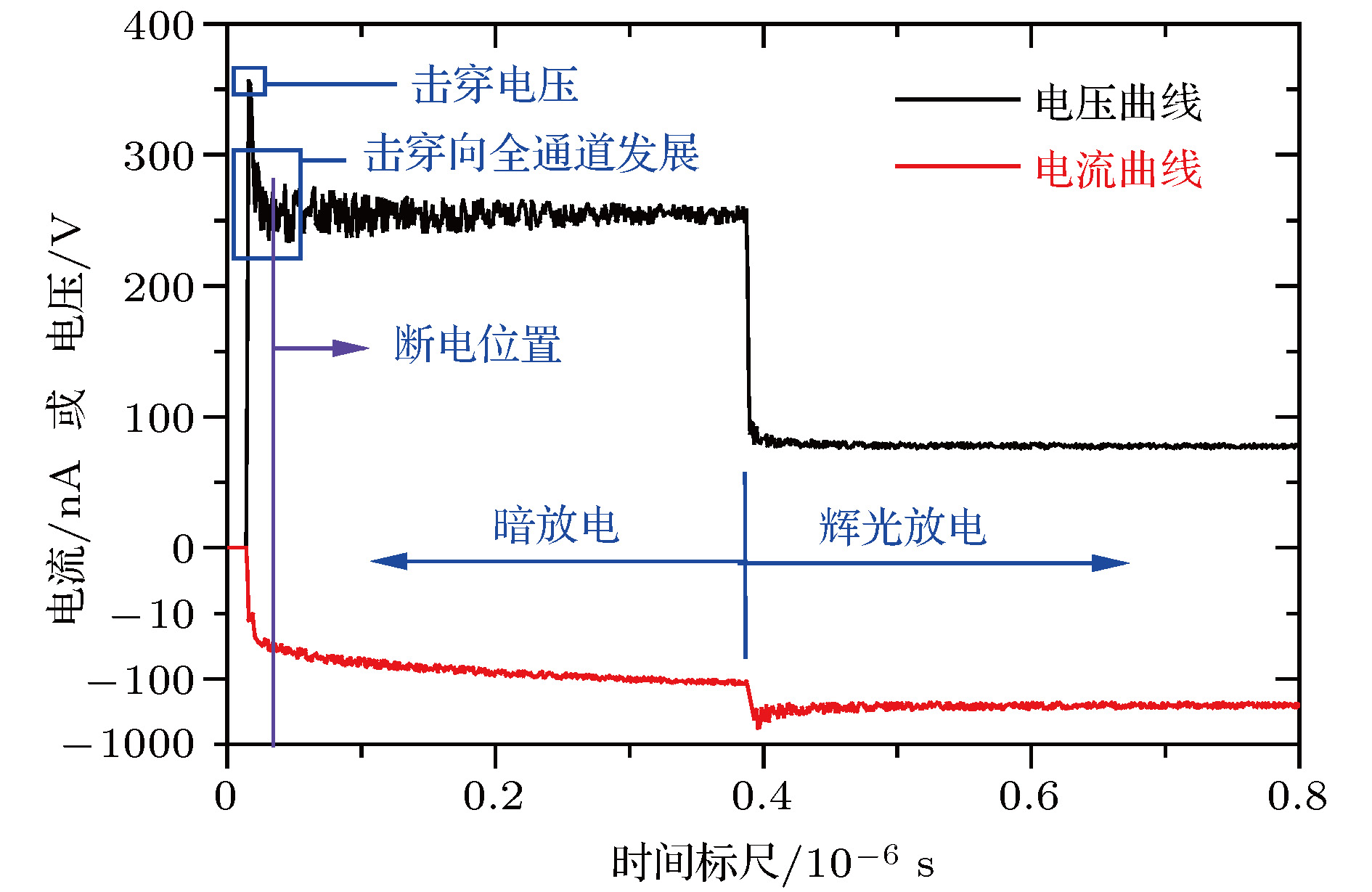图 6 放电过程的VI-t曲线(数据来自case 1工况)
Figure6. VI-t curve of the discharge process in case 1

图6中电压曲线的最高点就是起始击穿路径刚好发生击穿的时刻, 而采集到的电压数值就是击穿电压. 在起始路径的击穿刚触发后的0.05 ${\text{μ}}\rm{s}$内, 击穿电压会迅速下降, 并伴随电流的迅速上升, 这一段就是由起始路径局部击穿向全通道过渡的阶段, 因为放电路径的增多必然伴随电流升高, 因此, 只要在局部击穿完成后关闭电源, 就可以将电极间的放电严格控制在只有起始击穿路径击穿的阶段. 根据多次VI-t曲线的采集结果, 发现恰好进入暗放电的击穿电流(绝对值, 下同)在100 nA量级, 而汤森击穿刚好发生时的击穿电流在10 nA量级, 这说明应该将断电条件设定为“当击穿电流大于10 nA时, 断开电源输入”. 然而, “10 nA”的数值太小, 以致放电时间不充足, 在10³次量级的循环击穿试验中, 负电极表面很难形成明显痕迹, 因此, 经过多次调试, 如果断电条件中的击穿电流在50 nA时, 可以在10³次量级的循环击穿中对负电极表面留下较清晰的痕迹, 并且这些痕迹具有较高的指向性.
2 -->

3.2.仿真与试验结果对比

本文选取2种电极装置来验证DCP模型的计算精度: 圆片阶梯电极(case1)和磁等离子体动力学推力器(magneto-plasma dynamic thruster, MPDT, case2).
3 -->

3.2.1.Case 1

Case 1为圆片阶梯电极, 结构尺寸与候选路径划分见图7. 这里, 给出电场系数f, 以表征电极电场的不均匀程度(后文均有标注). 负电极表面的削蚀痕迹见图8(a), 击穿电压-间隙压强(V-p)曲线以及起始击穿路径的计算结果见图8(b).
图 7 圆片阶梯电极的结构及候选路径划分(f = 3.97)
Figure7. The geometry and potential path generation in the laddered plate electrode (f = 3.97)

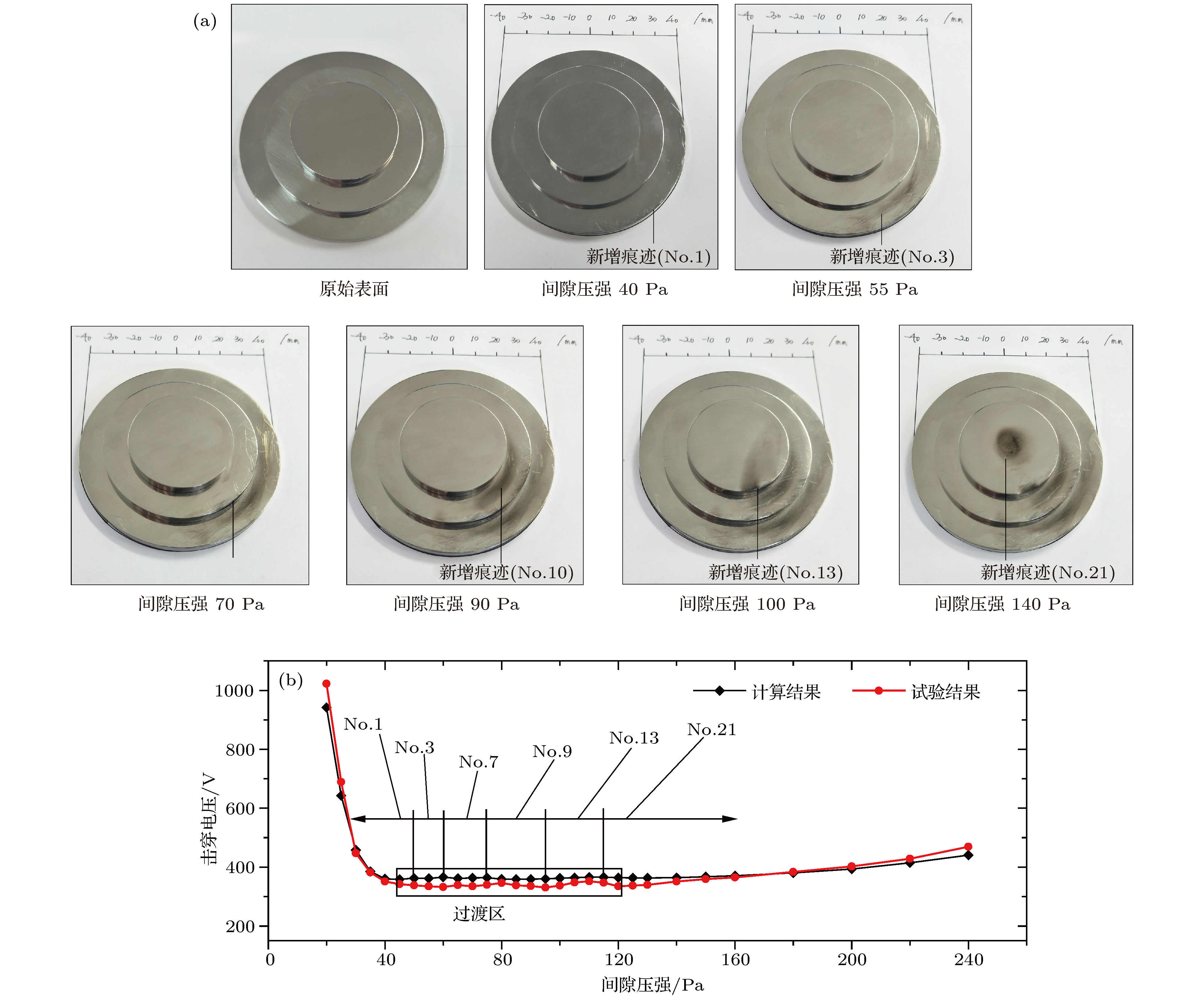图 8 Case 1试验与计算结果对比(气体工质: Xe)
Figure8. The comparison of the calculation and test results in case 1 (working medium: Xe)

根据图8(a), 这里进行2点关于试验现象的说明: 第一, 由于不锈钢电极含C元素, 在负电极表面削蚀过程中会产生一定的C原子沉积, 因此电极表面某些位置会有黑色痕迹(而case 2的负电极为W, 所以并没有这种黑色痕迹); 第二, 由于电极加工精度以及两电极安装的平行度难以达到绝对标准, 所以原本应在回转体电极一周都出现的削蚀痕迹, 只出现在某些局部位置, 但这些位置依然可以指向起始击穿路径. 根据试验结果, 我们发现负电极表面的新增痕迹趋势会随着间隙压强的变化而变化, 与Osmokrovic描述的临界区域变化的现象基本相符. 并且, 虽然电极表面痕迹所指向的起始路径与计算结果不完全一一对应, 但所呈现的路径转移趋势与计算结果可以保持定性一致. 在击穿电压的计算方面(图8(b)), DCP在case1的计算相对误差在0.56%—5.88%, 尤其在起始击穿路径转移的过渡区, 可基本捕捉击穿电压的变化趋势.
3 -->

3.2.2.Case 2

Case 2为MPDT的击穿工况, MPDT属于电推进动力装置, 本文的MPDT采用20 kW级、推力为600 mN的原理样机, 该样机的应用平台为高轨XX卫星的轨道转移推进系统. MPDT的点火过程起始于阴极管与阳极环之间的击穿, 当放电足以令钨阴极管达到热发射温度时, MPDT则迅速进入稳定工作状态. 推力器的电极结构和候选路径划分见图9, 负电极(阴极管)表面的痕迹结果及击穿电压-气体流率(V-fr)曲线见图10. 其中, 气体工质为Ar, 关于Ar的碰撞截面公式见文献[20], Ar与其它材料负电极的二次电子发射系数见文献[21].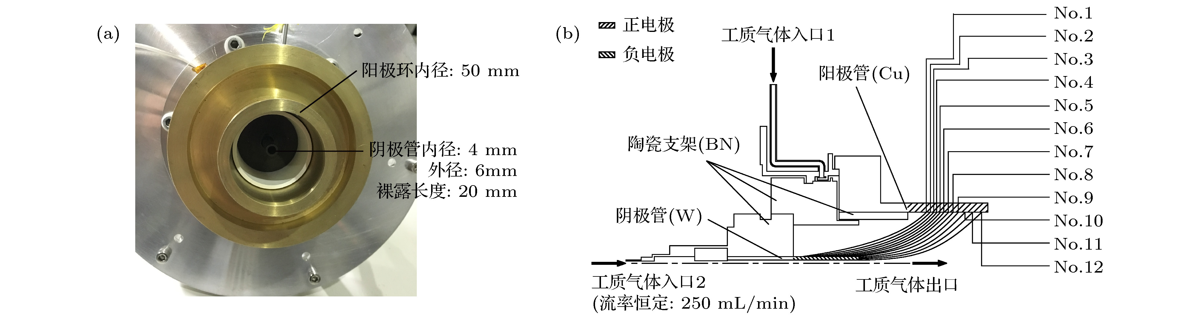
图 9 MPDT电极的相关信息　(a)实物照片; (b)电极结构及候选路径划分(f = 2.47)
Figure9. The relevant information of the MPDT: (a) Physical photograph; (b) the electrode geometry and potential path generation

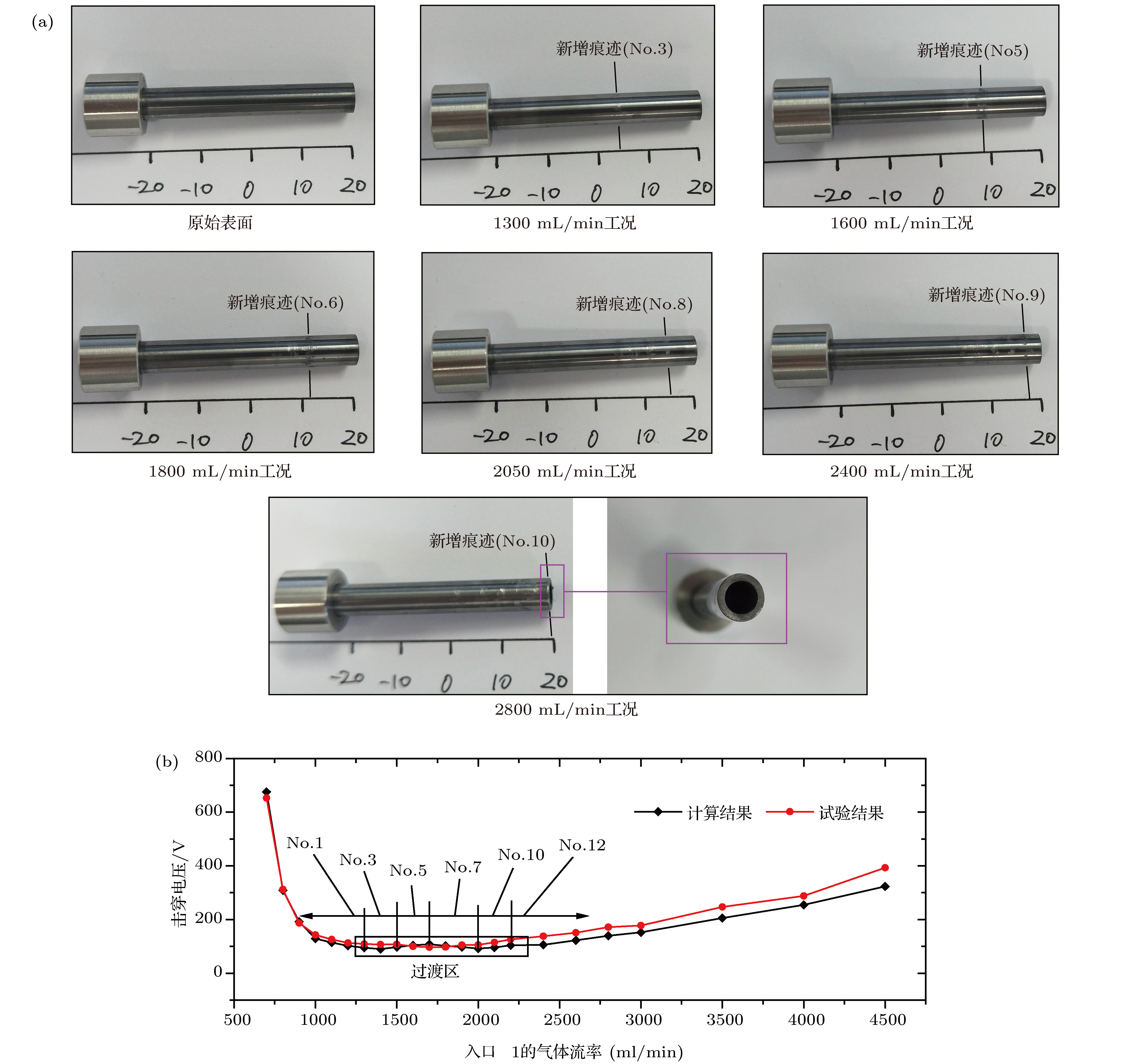图 10 Case 2试验与计算结果对比(气体工质: Ar)
Figure10. The comparison of the calculation and test results in case 2 (working medium: Ar)

据图10, 同样地, 负电极表面的新增痕迹趋势与起始路径计算结果的趋势在定性层面保持一致, 并且, 击穿电压的计算相对误差在0.42%—7.90%.
综上, 通过试验与计算结果的对比, 可以初步证实: 第一, 起始击穿路径确实会发生转移; 第二, DCP模型能够从定性角度捕捉起始击穿路径的转移方向.

前文对DCP模型的计算精度进行了初步验证, 并通过case 1和case 2的结果展示出起始击穿路径的相关特性. 为进一步研究起始路径的这种特性, 本节将给出其他4种比较有代表性的电极结构, 以归纳出起始路径转移的普遍规律.
2

-->

4.1.case 3

Case 3为两非平行直板电极间的击穿工况, 如图11(a)所示, 电极在入纸面方面为无限长, 两电极结构完全相同, 计算结果见图11(b).
图 11 Case 3的计算输入条件及计算结果(气体工质: Xe)　(a)电极结构及候选路径划分(f = 2.45); (b)V-p曲线的计算结果及起始路径分布
Figure11. The input conditions and calculation results in case 3 (working medium: Xe): (a) The electrode geometry and potential path generation; (b) the calculation results of the V-p curve and the critical path distribution

2 -->

4.2.Case 4

Case 4为无加热器空心阴极(heaterless hollow cathode, HHC)的工况. 在HHC点火过程中, 阴极管-触持极间会首先引发气体击穿, 通过离子轰击负电极表面而加热发射体, 使发射体达到工作温度(1300 K左右), 然后在阴极管-阳极板间进行稳定放电(阳极板在触持极右侧2—3 cm, 图12(a)未展示). 因此, HHC的点火性能主要依赖于气体击穿过程. HHC击穿所发生的正负电极结构见图12(a), 计算结果见图12(b).
图 12 Case 4的计算输入条件及计算结果(气体工质: Xe)　(a)电极结构及候选路径划分(f = 3.76); (b)V-fr曲线的计算结果及起始路径分布
Figure12. The input conditions and calculation results in case 4(working medium: Xe): (a) The electrode geometry and potential path generation; (b) the calculation results of the V-p curve and the critical path distribution

2 -->

4.3.case 5

Case 5为两平行圆柱电极间的击穿工况, 电极在入纸面方面为无限长, 2个电极结构完全相同(图13(a)), 计算结果如图13(b). 气体工质为Ar.
图 13 Case 5的计算输入条件及计算结果(气体工质: Ar): (a) 电极结构及候选路径划分(f = 3.43); (b) V-p曲线的计算结果及起始路径分布
Figure13. The input conditions and calculation results in case 5 (working medium: Ar): (a) The electrode geometry and potential path generation; (b) the calculation results of the V-p curve and the critical path distribution

2 -->

4.4.case 6

Case 6为圆柱-直板电极间的击穿工况, 两电极在入纸面方向无限长, 并且, 两电极的中心轴线平行. 电极结构及候选路径划分见图14(a), 计算结果见图14(b). 气体工质为Xe.
图 14 Case 6的计算输入条件及计算结果(气体工质: Xe)　(a)电极结构及候选路径划分(f = 2.84); (b)V-p曲线的计算结果及起始路径分布
Figure14. The input conditions and calculation results in case 6(working medium: Xe): (a) The electrode geometry and potential path generation; (b) the calculation results of the V-p curve and the critical path distribution

综上, 通过对case 1到case 6的对比分析, 发现这6个工况的计算或试验结果都存在一些共有的特性:
(1)在压强或气体流率上升过程中, 起始击穿路径并不是固定不变的, 会发生转移;
(2)在V-p曲线或V-fr曲线中, 曲线形貌与经典Paschen曲线不同, 在曲线的左支和右支中间总会存在一个过渡区, 其击穿电压会表现出“上下波动, 近似持平”的特性;
(3)起始击穿路径的转移方向总是表现为从较长路径向较短路径转移.

结合试验与仿真结果来看, 上述关于起始击穿路径的特性不应认为是一个巧合, 在以往****的研究中^[4,5,22-24], 也确实在击穿试验中观察到了相似的试验结果. 因此, 本节将深入讨论上述两个特性的内在机理.
2

-->

5.1.路径转移原因和过渡区特性

以case 3为例, 利用DCP模型将case 3所有候选击穿路径的V-p曲线都计算出来, 并与整个电极的V-p曲线放在一起做对比(图15).
图 15 整个电极的V-p曲线形成原因(case 3)
Figure15. The formation reason of the entire V-p curve in the whole gap of case 3

图15所展示的蓝色细线为没有成为起始路径的候选路径的曲线, 而每一条红色细线为各起始击穿路径的曲线, 黑色粗线为整个电极的曲线(图11(b)的计算结果). 据图15, 并不是所有候选路径都有机会成为起始击穿路径, 只有那些可以达到全通道路径中最低V-p曲线的路径才能成为起始击穿路径, 并且, 每条起始路径都仅仅在某个压强范围内具备成为当前起始击穿路径的条件, 而在其他压强范围内则不具备条件, 所以, 当压强或气体流率变化时, 起始击穿路径就会轮流更替, 发生“频繁的路径转移”. 另一方面, 能够成为起始击穿路径的候选路径, 只能将自身V-p曲线的最优部分贡献给整个电极的V-p曲线. 例如, No.21将其左支贡献给黑色曲线, No.1将其右支贡献给黑色曲线, 而No.14, No.10, No.8, No.4和No.1会在60—190 Pa之间轮流将自身的最小电压区域(Paschen定律中称之为(pd)_min区域)贡献给黑色曲线的过渡区. 因而, 过渡区每条起始路径的(pd)_min区域在电压值上都是比较接近的, 取决于放电气体种类和电极材料. 因此, 过渡区的击穿电压会表现出“上下波动, 近似持平”的特性, 直到起始路径转移到最后一条路径时, 曲线才会继续上升.
2 -->

5.2.路径转移方向

根据DCP数值模型, 判断起始路径的核心参数为每条候选路径的总的二次电子发射数量n_γ, 而影响该参数的直接因素为每条候选路径的总电离次数. 因此, 为揭示路径转移规律, 这里先给出不同压强下, 各路径中所引发的电离碰撞次数分布. 依然以case 3为例, 选择No.18代表长路径, No.4代表段路径(参考图11(a)), 选择p = 40 Pa为低气压工况, p = 80 Pa为高气压工况. 利用DCP模型, 将每个计算节点的电离次数统计成云图(图16).
图 16 不同压强下电极间隙的电离碰撞次数分布(case 3)　(a) p = 40 Pa; (b) p = 80 Pa
Figure16. The ionization collision number distribution at different gap pressures in case 3: (a) p = 40 Pa; (b) p = 80 Pa

根据图16, 发现在p = 40 Pa时, No.18的电离次数确实高于No.4, 在No.18附近有明显的电子雪崩形态; 而在p = 80 Pa时, 情况正好相反. 接着, 按照电离碰撞概率公式(第2节的8(b)式), 有4个参数会影响电离概率P_ion: ${N_{\rm{n}}}$, ${\sigma _T}\left({E_{{k},e}}\right)$, $\Delta l$和${\sigma _{{\rm{ion}}}}\left({E_{{k},e}}\right)/{\sigma _T}\left({E_{{k},e}}\right)$. ${N_{\rm{n}}}$与间隙压强有直接关系, ${\sigma _T}\left({E_{{k},e}}\right)$和${\sigma _{{\rm{ion}}}}\left({E_{{k},e}}\right)/{\sigma _T}\left({E_{{k},e}}\right)$与电子动能有关, 而$\Delta l$与路径长度有直接关系. 那么, 对于case 3来说, 整个电极间隙都共享相同的${N_{\rm{n}}}$, 如果${\sigma _T}\left({E_{{k},e}}\right)$和${\sigma _{{\rm{ion}}}}\left({E_{{k},e}}\right)/{\sigma _T}\left({E_{{k},e}}\right)$不变, 则长路径的P_ion将一直高于短路径, 起始击穿路径将永远是最长路径, 而不应该转移. 显然, 这与试验结果不符, 由此来推断, 应该是在不同的间隙压强下${\sigma _T}\left({E_{{k},e}}\right)$和${\sigma _{{\rm{ion}}}}\left({E_{{k},e}}\right)/{\sigma _T}\left({E_{{k},e}}\right)$发生了变化. 因此, 下一步将继续研究${\sigma _T}\left({E_{{k},e}}\right)$, ${\sigma _{{\rm{ion}}}}\left({E_{{k},e}}\right)/{\sigma _T}\left({E_{{k},e}}\right)$和${E_{{k},e}}$这3个参数在沿No.4和No.18路径上的分布情况(图17). 由于各计算节点的电子数量较多, 各电子的动能也不同, 所以图17统计上述3个参数在各节点的平均值.
图 17 ${\sigma _T}\left({E_{{k},e}}\right)$, ${\sigma _{{\rm{ion}}}}\left({E_{{k},e}}\right)/{\sigma _T}\left({E_{{k},e}}\right)$和${E_{{k},e}}$在不同压强、不同候选路径上的分布规律(case 3)　(a)平均${\sigma _T}\left({E_{{k},e}}\right)$, p = 40 Pa; (b)平均${\sigma _T}\left({E_{{k},e}}\right)$, p = 80 Pa; (c)平均${\sigma _{{\rm{ion}}}}\left({E_{{k},e}}\right)/{\sigma _T}\left({E_{{k},e}}\right)$, p = 40 Pa; (d)平均${\sigma _{{\rm{ion}}}}\left({E_{{k},e}}\right)/{\sigma _T}\left({E_{{k},e}}\right)$, p = 80 Pa; (e)平均${E_{{k},e}}$, p = 40 Pa; (f)各节点的平均${E_{{k},e}}$, p = 80 Pa
Figure17. The distribution of ${\sigma _T}\left({E_{{k},e}}\right)$,${\sigma _{{\rm{ion}}}}\left({E_{{k},e}}\right)/{\sigma _T}\left({E_{{k},e}}\right)$ and ${E_{{k},e}}$ at different gap pressures and different potential paths in case 3: (a) The average ${\sigma _T}\left({E_{{k},e}}\right)$, p = 40 Pa; (b) the average ${\sigma _T}\left({E_{{k},e}}\right)$, p = 80 Pa; (c) the average ${\sigma _{{\rm{ion}}}}\left({E_{{k},e}}\right)/{\sigma _T}\left({E_{{k},e}}\right)$, p = 40 Pa; (d) the average ${\sigma _{{\rm{ion}}}}\left({E_{{k},e}}\right)/{\sigma _T}\left({E_{{k},e}}\right)$, p = 80 Pa; (e) the average ${E_{{k},e}}$, p = 40 Pa; (f) the average ${E_{{k},e}}$, p = 80 Pa

据图17(a)—(d), 在低气压下, No.4和No.18的${\sigma _T}\left({E_{{k},e}}\right)$和${\sigma _{{\rm{ion}}}}\left({E_{{k},e}}\right)/{\sigma _T}\left({E_{{k},e}}\right)$分布并没有显著区别, 但是高气压下, No.4的${\sigma _T}\left({E_{{k},e}}\right)$和${\sigma _{{\rm{ion}}}}\left({E_{{k},e}}\right)/$$ {\sigma _T}\left({E_{{k},e}}\right)$要明显高于No.18. 形成该趋势的直接原因可以由图17(e)和图17(f)解释, 即No.4和No.18的电子动能在低气压下相当, 但在高气压下No.18的电子动能明显低于No.4. 接着, 这里继续分析导致电子动能变化的原因: 能够影响电子动能降低的因素除了电离碰撞以外, 就是激发碰撞. 因而, 图18给出每个计算节点的激发碰撞次数分布.
图 18 不同压强下电极间隙的激发碰撞次数分布(case 3)　(a) p = 40 Pa; b) p = 80 Pa
Figure18. The excitation collision number distribution at different gap pressures in case 3: (a) p = 40 Pa; (b) p = 80 Pa

图18显示: 在低气压工况中, 整个通道各候选路径的激发碰撞次数几乎相同, 并且碰撞次数较少, 这导致各个路径的电子动能损失都较少, 于是就形成了图17(e)的趋势(No.4和No.18的电子动能相当); 但在高气压工况中, 激发碰撞次数在长路径上明显增多, 这是由于长路径的$\Delta l$较高, 其触发的激发碰撞概率将明显高于短路径, 从而导致长路径的电子动能损耗较大, 于是形成了图17(f)的趋势.
综上, 激发碰撞所导致的能损影响是起始路径转移的关键因素: 在低气压下, 激发碰撞在各路径的发生次数都较低, 其影响程度较小, 那么较长的路径更容易触发击穿; 但随着气压升高时, 激发碰撞在长路径中的发生次数明显升高, 其影响程度逐渐增加, 就导致起始路径逐渐从长路径向短路径转移.

本文在先前****的研究基础上, 采用数值模型(DCP)与试验相结合的方法, 对低气压起始击穿路径问题进行研究, 初步获得稍不均匀电场(f = 2.0—4.0)中, 起始击穿路径的存在位置规律以及相关机理:
1)在间隙压强或气体流率发生变化时, 起始击穿路径会发生转移, 这与Osmokrovic的试验结果吻合. 通过计算分析, 本文认为, 路径转移与每条候选路径各自的击穿电压曲线特性有关, 整个电极通道总会在不同工况下选择最可能发生击穿的那条路径来引发击穿, 因此, 起始击穿路径会在不同压强或流率工况下发生转移;
2)在V-p或V-fr曲线中, 曲线左支和右支之间总会存在一个过渡区, 过渡区的击穿电压会表现出上下波动、近似持平的变化趋势, 原因为过渡区的各起始击穿路径将其(pd)_min部分贡献给整个通道的击穿曲线, 而这些(pd)_min区域的击穿电压在数值上接近, 导致过渡区的曲线特性出现上下波动、近似持平, 只有转移到最后一条起始击穿路径后, 曲线才会上升;
3)当间隙压强或流率从低到高增加时, 起始路径的转移方向总会沿着较长路径向较短路径转移, 这是因为较低气压下各候选路径的激发碰撞次数均较少, 电子动能较高, 电离概率主要受路径长度影响, 击穿会选择较长路径, 而在较高气压下, 较短路径的激发碰撞次数明显低于较长路径, 其能损较低, 更易引发击穿.