HTML
--> --> -->It has been shown that as the most important interannual mode, ENSO can exert a great impact on global climate (Wallace and Gutzler, 1981; Alexander et al., 2002). While the impact on midlatitudes during ENSO mature winters is primarily through the Pacific-North America (PNA) pattern, Indian monsoon precipitation is influenced through suppressed anomalous heating over the Maritime Continent during the El Ni?o developing summer, and East Asia precipitation is influenced through an anomalous anticyclone in the western North Pacific (WNPAC) during the El Ni?o decaying summer (Wang et al., 2003; Li and Wang, 2005). The maintenance of the WNPAC results from local air-sea interaction in the western North Pacific (WNP) (Wang et al., 2000, 2002; Wu et al., 2010) or remote Indian Ocean (IO) forcing during the El Ni?o decaying summer (Xie et al., 2009; Wu et al., 2010). Remote IO forcing can drive a warm equatorial Kelvin wave to its east with easterly wind anomalies, inducing surface divergence and suppressing deep convection in the subtropical WNP, thus forming the WNPAC. This process is called the IO capacitor effect (Xie et al., 2009). Wu et al. (2010) further confirmed that both the local cold sea surface temperature anomalies (SSTAs) in the WNP and the remote SSTA forcing in the tropical IO are important in maintaining the WNPAC. Chen et al. (2016) showed that during a rapid El Ni?o-La Ni?a transition, central-eastern Pacific cooling plays an important role in maintaining the WNPAC. Various theories have been proposed to explain the formation and maintenance of the WNPAC (see Li et al., 2017 for a thorough review on this topic). A suppressed heating anomaly associated with the WNPAC may strengthen mei-yu rainfall through anomalous moisture transport (Chang et al., 2000a), forming a so-called Pacific–Japan (PJ) pattern (Nitta, 1987; Kosaka and Nakamura, 2006) or East Asia–Pacific (EAP) pattern (Huang and Li, 1988).
Note that the ENSO–East Asian rainfall relationship is unstable, and the diversity of ENSO intensity, evolution, and type can lead to different East Asian summer rainfall characteristics (Yuan and Yang, 2012; Wang et al., 2017a). This relationship is also modulated by the zonal shifting of the WNPAC (Piao et al., 2020), periodicity of the PJ pattern interannual variability (Chen and Zhou, 2014), the summer mean state, and the teleconnection pattern excited by Indian summer rainfall (Wang et al., 2017a). East Asian subtropical frontal rainfall is sensitive to the strength and location of the western Pacific subtropical high (WPSH), which is largely determined by the local atmosphere–ocean interaction (Wang et al., 2017a). Some studies have further shown that the origins and predictabilities of East Asia rainfall in early summer and late summer are obviously different (Wang et al., 2009; Xing et al., 2016, 2017).
Besides tropical forcing, East Asian climate can also be influenced by midlatitude circulation changes. For example, a circumglobal teleconnection (CGT) pattern has been observed during midlatitude northern hemispheric summer, and it exerts a great impact on rainfall and temperature in East Asia (Ding and Wang, 2005). The CGT pattern may be triggered by heating anomalies over the Indian summer monsoon, ENSO forcing (Ding and Wang, 2005; Ding et al., 2011), and the convection patterns near the northern Indian Ocean (Chen and Huang, 2012) and the eastern Mediterranean (Yasui and Watanabe, 2010). The CGT pattern has also been observed on the interdecadal timescale and is likely a dominant interdecadal mode in boreal summer over the Northern Hemisphere, possibly triggered by the Atlantic Multidecadal Oscillation (Lin et al., 2016; Wu et al., 2016). Over the Eurasian Continent sector, the CGT pattern overlaps with a so-called Silk Road Pattern (SRP) (Enomoto et al., 2003; Lu et al., 2002), which extends along the summer westerly jet (40°N) from central Asia to East Asia, and this exerts great impacts on East Asian climate during early and late summer (Hong et al., 2018). Chen and Huang (2012) pointed out that the CGT could be considered as the interannual component of the SRP. Previous studies have shown that the SRP could be excited by Indian summer monsoon heating (Wu, 2002; Enomoto et al., 2003; Enomoto, 2004; Liu and Ding, 2008) and northern Indian Ocean heating (Chen and Huang, 2012). Other studies have suggested that the SRP may be an internal atmospheric mode (Sato and Takahashi, 2006; Kosaka et al., 2009; Yasui and Watanabe, 2010; Chen et al., 2013).
Historically, extreme summer precipitation over the YRV (such as that in 1983, 1998, and 2016) has always happened during the decaying summer of super eastern Pacific (EP) El Ni?o events. Surprisingly, the YRV rainfall in June-July 2020 was record-breaking, exceeding total rainfall amounts in 1983, 1998, and 2016, even though a moderate CP type El Ni?o occurred in the preceding winter. What caused the extreme rainfall over the YRV in summer 2020? The present study aims to answer this question.
The objective of the present study is to reveal the fundamental cause of the extreme precipitation over the YRV. Observational data analysis and idealized numerical model experiments are carried out to address the aforementioned scientific question. The remaining paper is organized as follows. The data, method, and model are introduced in section 2. In section 3, we describe the observational characteristics of key atmospheric circulation anomalies in the tropical and midlatitudes associated with the June-July 2020 extreme rainfall anomaly. Specific processes through which tropical and midlatitude circulation anomalies form are discussed in sections 4 and 5, respectively. Finally, the conclusion and discussion are given in section 6.
To separate the interannual and interdecadal components, the 42-yr anomaly time series is subject to a 13-yr running mean to extract its interdecadal/trend component. An interannual component is then obtained by subtracting the interdecadal/trend component from the original 42-yr anomaly time series. Considering the missing values on both ends of the time series, two filtering methods are employed. In Method 1, 13 points are used for a running average in the middle of the time series, while less points are used at the starting and ending portions of the time series. In Method 2, only the point and its preceding 6 points are used from the 7th point to the ending point (Hsu et al., 2015; Zhu and Li, 2015) to extract the 13-yr running mean.
The moist static energy (MSE) is calculated to describe potential atmospheric convective instability. It is defined as the linear function of atmospheric temperature, moisture, and geopotential height (Neelin and Held, 1987; Wang et al., 2017b).


An atmospheric general circulation model, ECHAM version 4.6 (ECHAM4.6), that was developed at the Max-Plank Institute for Meteorology (Roeckner et al., 1996) is applied in the present study to investigate the relative roles of tropical heating anomalies in causing atmospheric circulation responses. The model is run with a 2.8°

| Experiments | Description |
| CTRL | Forced by global climatological SST |
| EXP_All | Forced by global climatological SST plus an additional positive diabatic heating anomaly over the Indian Ocean (20°S–25°N, 40°–135°E) and a negative diabatic heating anomaly over the tropical Pacific (10°S–15°N, 135°E–100°W) |
| EXP_IO | Forced by global climatological SST plus an additional positive diabatic heating anomaly over the Indian Ocean (20°S–25°N, 40°–135°E) |
| EXP_TP | Forced by global climatological SST plus an additional negative diabatic heating anomaly over the tropical Pacific (10°S–15°N, 135°E–100°W) |
| EXP_IM | Forced by global climatological SST plus an additional positive diabatic heating anomaly over the Indian monsoon region (8o–25oN, 60o–85oE) |
| EXP_TA | Forced by global climatological SST plus an additional positive diabatic heating anomaly over the tropical Atlantic (0o–15oN, 60o–10oW) |
| EXP_EP | Forced by global climatological SST plus an additional positive diabatic heating anomaly over the eastern Pacific (5o–15oN, 180o–100oW) |
Table1. List of numerical experiments conducted with ECHAM4.6.
The heating specified in the model experiments is transferred from precipitation anomaly according to the following equation:
where


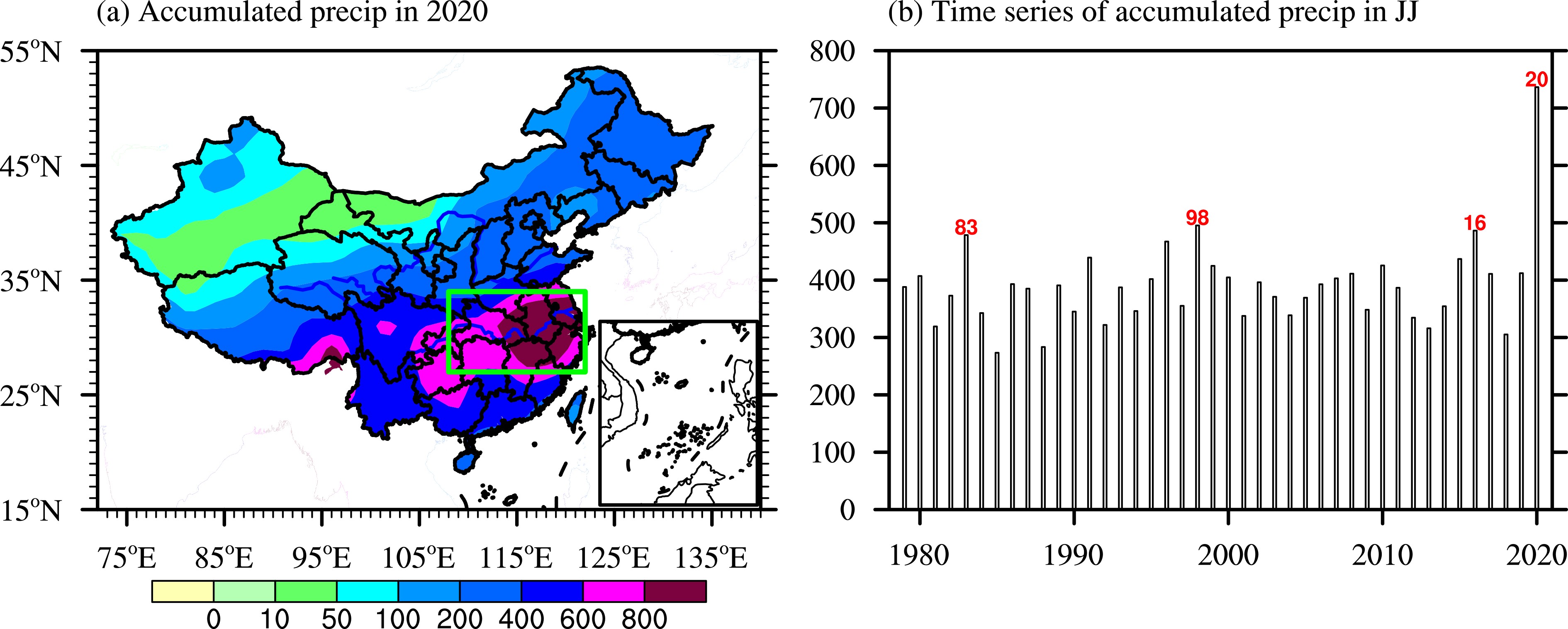 Figure1. (a) Accumulated precipitation (mm) from 1 June to 31 July 2020 over China and (b) time series of the accumulated precipitation (mm) during June-July averaged over the Yangtze River Valley (green box, 27°–34°N, 108°–122°E).
The most notable feature of anomalous circulation in JJ 2020 is a large-scale low-level anticyclone in the tropical WNP south of the mei-yu rainband (Figs. 2a, b). Southerly wind anomalies to the west of the anticyclone advected warm and moist air northward, converging into the mei-yu front. Due to the warm advection and the strong solar radiation associated with less precipitation, positive surface air temperature anomalies appeared south of the YRV.
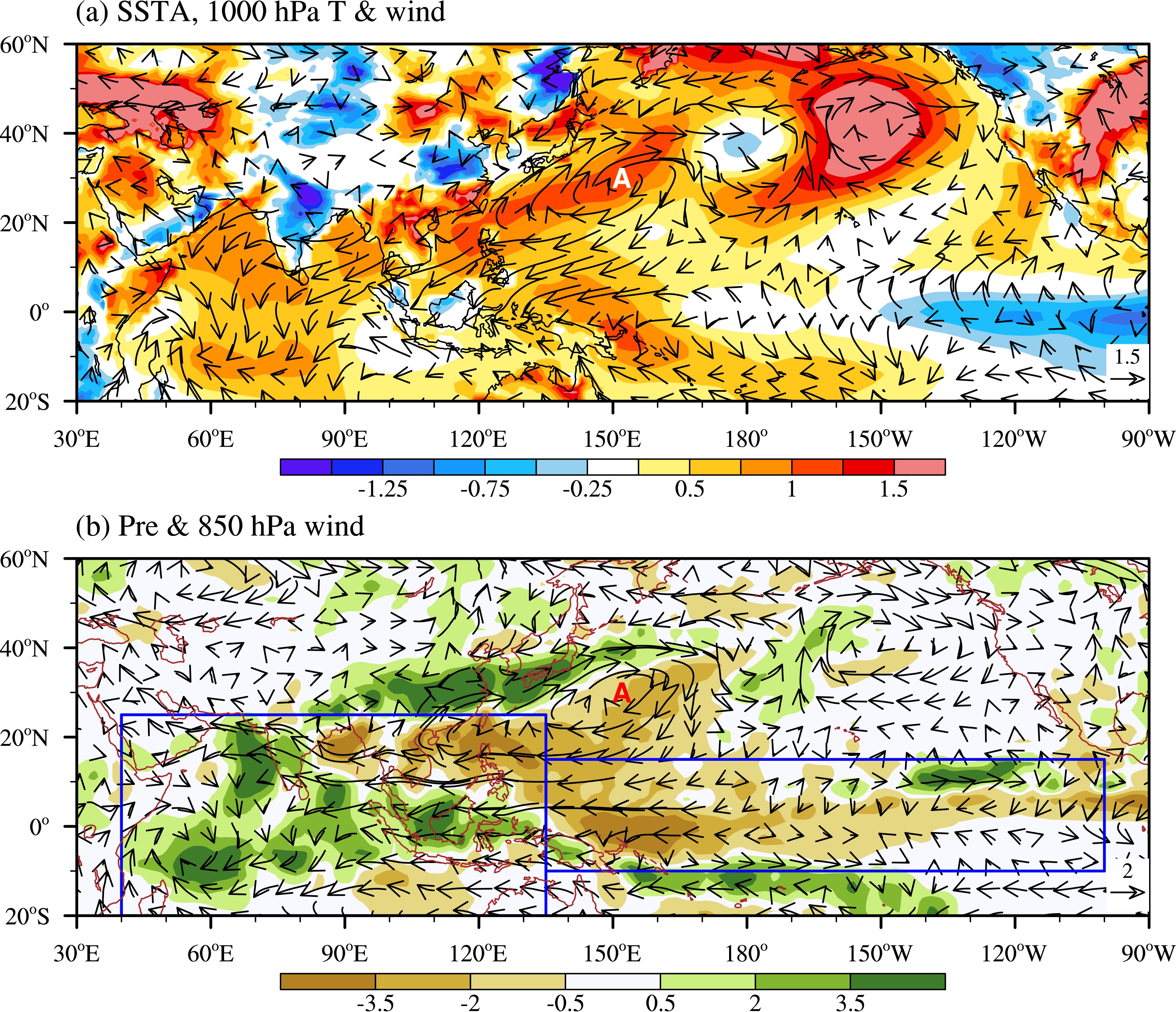 Figure2. The horizontal patterns of (a) anomalous SST (shading in ocean; °C) and air temperature (shading in land; °C) and horizontal wind (vector; m s?1) at 1000 hPa and (b) anomalous precipitation (shading; mm d?1) and horizontal wind at 850 hPa (vector; m s?1) in JJ (June?July) 2020. The baseline for the mean climatology is based on the 1979–2020 period. Letter “A” denotes the anomalous anticyclone center in the WNP.
Another notable feature is a cold surface temperature anomaly north of the YRV (Fig. 2a). The cold anomaly resulted from cold advection by northeasterly anomalies in Northeast Asia (NEA, Fig. 3a). The maintenance of the dipole pattern of the anomalous temperature advection strengthened the meridional temperature gradient and led to a persistent and strong mei-yu front. Accompanied with the dipole pattern of the anomalous temperature advection was a similar dipole pattern of anomalous moisture advection, as seen from Fig. 3b.
 Figure3. The horizontal patterns of anomalous (a) advection of mean temperature by anomalous wind at 1000 hPa (shading; ×10?5 °C s?1) superposed by 1000 hPa wind anomaly field (vector; m s?1), (b) advection of mean moisture by anomalous wind (shading; ×10?5 g kg?1 s?1) superposed by the anomalous wind field at 1000 hPa (vector; m s?1), (c) moist static energy (J kg?1) integrated from 1000 hPa to 850 hPa, and (d) precipitation (shading; mm d?1) and specific humidity at 925 hPa (contour; g kg?1) averaged during JJ 2020.
Because of the configuration of the temperature advection and moisture advection, a great north-south contrast between dry and cold conditions north of the YRV and wet and warm conditions south of the YRV can clearly be seen in the vertically integrated (1000–850 hPa) MSE field (Fig. 3c). The confrontation of the high MSE air to the south and the low MSE air to the north persisted for a two month period, leading to a stationary mei-yu front and thus devastating floods over the middle and lower reaches of the YRV (Fig. 3d).
Typically, the mei-yu rainband occurs over the YRV for a two-week period, and then it moves northward. A key scientific question around the 2020 flood asks why the anomalous circulation and rainband persist for a two-month period. Given that the atmospheric circulation itself does not have a long memory, one needs to pay attention to the oceanic forcing. Note that a La Ni?a-like SSTA pattern appeared in the equatorial Pacific and a warm SSTA occurred over the tropical Indian Ocean (IO) basin (Fig. 2a). In the following section, we will examine how these SSTAs and associated atmospheric heating conditions may affect the tropical and midlatitude circulation anomalies.
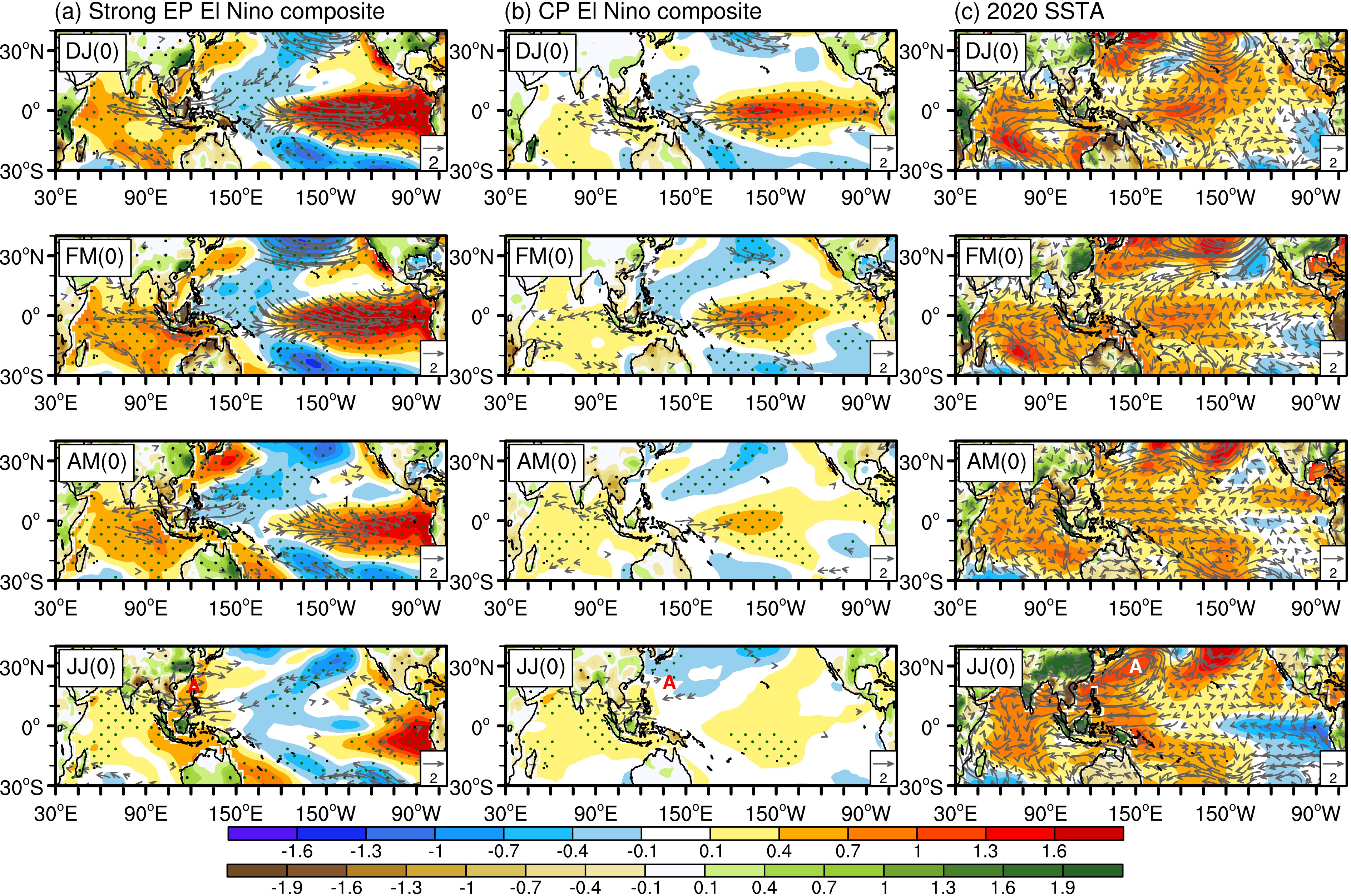 Figure4. Bi-monthly pattern evolutions of anomalous SST (shading in ocean; °C), precipitation (shading in land; mm d?1) and 850 hPa wind fields (vector; m s?1) for (a) the strong EP El Ni?o composite (left panel), (b) the CP El Ni?o composite (middle panel), and (c) the 2020 event (righ panel). Dots in ocean (land) show the SSTA (precipitation) values passing the confidence level of 95% using bootstrap test. The vector is shown only when the u-wind or v-wind exceeds 95% confidence level. The notation “(0)” indicates the decay year of the El Ni?os. Letter “A” in JJ(0) represents the anomalous anticyclone center in the WNP.
An important difference between the SEP and CP El Ni?o composites (Figs. 4a, b) is the SSTA evolution in the equatorial Pacific. While there is a quick phase transition of the SSTA from a positive to a negative value in the central Pacific during SEP, the SSTA decays at a much slower rate in the CP El Ni?o composite. As a result, a positive SSTA still appears in the equatorial central Pacific in JJ(0). Such a quick phase transition of the SSTA has an important impact on the strengthening of the WNPAC (Wang et al., 2013). A cold SSTA in the central equatorial Pacific would induce negative diabatic heating in situ, which could further induce an anomalous anticyclone to its northwest, as a Gill (1980) model response. In fact, this is a partial reason as to why the anomalous anticyclone is much stronger in JJ in Fig. 4a compared to Fig. 4b.
Another noted feature includes much stronger IO basin warming during SEP El Ni?os than during CP El Ni?os. The warmer IO could induce a greater basin-wide heating anomaly and cause a Kelvin wave response to its east (Gill, 1980). The anticyclonic shear of the Kelvin wave easterly winds, through the interaction with the WNP summer monsoon, would lead to a suppressed convection anomaly and thus forming the WNPAC (Wu et al., 2010). Therefore, the stronger IO warming during SEP El Ni?os is also an important factor for the generation of a stronger WNPAC.
One may wonder whether the difference in the number of years for the composite analysis would affect the detection of fast/slow phase transition of SSTAs, but the evolution of SSTAs during each CP and SEP El Ni?o case (figure not shown) indicates that the phase transition of most CP El Ni?o cases is indeed slower than that of most SEP El Ni?o cases.
The argument above suggests that both the quick phase transition in the Pacific and the enhanced IO warming were responsible for generating a stronger WNPAC during the SEP El Ni?o. The stronger WNPAC in JJ further induced a stronger precipitation anomaly over the YRV through greater moisture transport. A greater rainfall anomaly in the SEP El Ni?o composite than that in the CP El Ni?o composite is clearly evident in Fig. 4.
What was unique about the SSTA evolution of the 2020 event? Figure 4c illustrates the SSTA pattern evolution from boreal winter to summer 2020. Note that a CP El Ni?o-like SSTA pattern appeared in the equatorial Pacific in December-January(0). Compared to the CP El Ni?o composite, the CP warming in early 2020 had similar strength. However, its horizontal pattern differed markedly; it was more like a Pacific Meridional Mode (PMM) pattern (Chiang and Vimont, 2004). The most important difference lies in the SSTA evolution. In contrast to the slow phase transition in the composite CP El Ni?o events, there was a quick phase transition of the SSTA in the equatorial Pacific in 2020. By JJ 2020, a cold SSTA occurred in the equatorial eastern Pacific. The amplitude of the cold SSTA in the tropical Pacific (Fig. 4c) was much greater than that of SEP El Ni?o composites (Fig. 4a). Meanwhile, the amplitude of the IO warming of the 2020 event was much greater than that of the CP El Ni?o composite and was comparable to that of the SEP El Ni?o composite. Despite a previous study showing that the tropical IO warming during El Ni?o decaying summer plays the dominant role in the maintenance of the WNPAC (Xie et al., 2009), here we emphasize that it is the combination of both the quick Pacific SSTA phase transition and the stronger than usual IO warming that led to a much stronger WNPAC and YRV floods in summer 2020 (Fig. 4c).
While a quick phase transition in the Pacific was possibly caused by the PMM-like SSTA pattern (Wang, 2018; Fan et al., 2020), it is unclear what caused a greater basin-wide warming in the IO. As seen from Fig. 4b, a relatively weak SSTA is associated with a CP El Ni?o. To unveil the cause of the unusually large IO warming in 2020, we decomposed the time series of the JJ SSTA averaged over the IO (17.5°S–25°N, 50°–90°E, green box shown in Fig. 5a) into an interannual and an interdecadal/trend component. As described in section 2, a 13-yr running mean was used in separating the two components. It is interesting to note that the large IO warming in 2020 was a result of the summation of the interannual and interdecadal/trend components (Fig. 5c) with an anomaly about 0.7°C warmer in JJ 2020. Regardless of which method was used, the two components are approximately equal. The result indicates that the exceptionally strong warming in the IO is part of an interdecadal and/or global warming signal. This result reminds us that it is necessary to consider the effect of the interdecadal mode and the global warming trend in real-time operational seasonal forecast (Zhu, 2018).
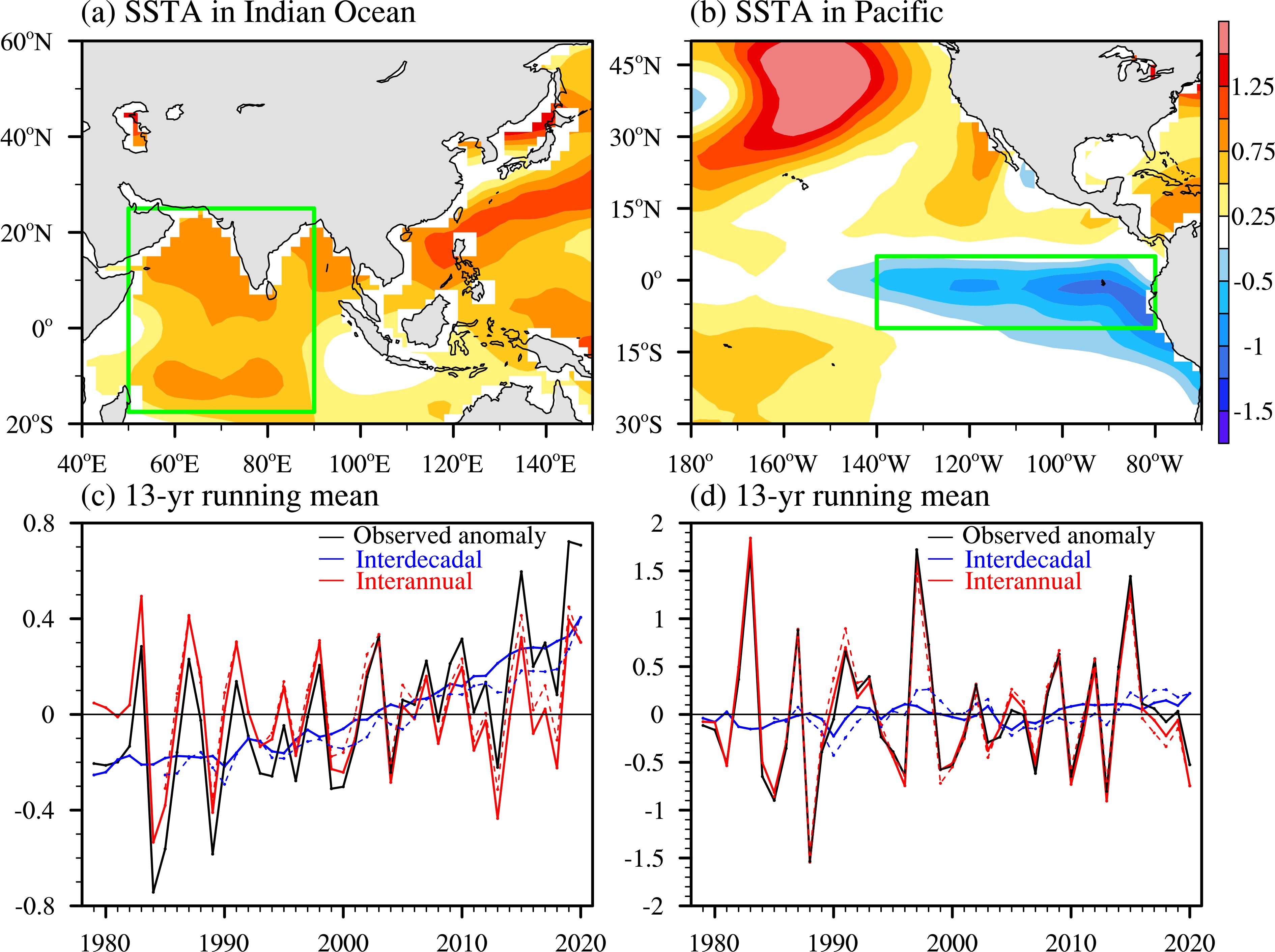 Figure5. The SSTA patterns (°C) in JJ 2020 over (a) the tropical Indian Ocean and (b) the eastern Pacific. (c) Time series of the observed SSTA (black lines; °C) averaged over the Indian Ocean box (17.5°S–25°N, 50°–90°E; green box in (a)) and its interannual (red lines; °C) and interdecadal/trend (blue lines; °C) components derived based on 13-yr running mean with Method 1 (solid lines) and Method 2 (dashed lines). (d) is similar to (c) but for SSTA averaged over the eastern Pacific box (10°S–5°N, 140°–80°W; green box in (b)).
One may wonder whether or not the Pacific SSTA in 2020 also involved the interdecadal/trend component. To answer that question, we calculated the interannual and interdecadal/trend components for the EP SSTA index shown in the right panel of Fig. 5. As one can see, the SSTA time series is primarily controlled by the interannual component, while the trend and interdecadal variation are relatively small. Therefore, it is concluded that the EP SSTA in 2020 was mainly attributed to its interannual variability while the IO SSTA was attributed to both the interannual and interdecadal/trend components.
To investigate the relative roles of the cold SSTA in the equatorial Pacific and the warm SSTA in the IO in contributing to the WNPAC, we conducted three sets of sensitivity experiments using ECHAM4.6. In the first experiment (EXP_IO), positive heating in the tropical IO and Maritime Continent (MC) sector (20°S–25°N, 40°–135°E) was specified. In the second experiment (EXP_TP), negative heating in the tropical Pacific (TP; 10°S–15°N, 135°E–100°W) was specified. The heating regions are represented by the blue boxes shown in Fig. 2b. In the third experiment (EXP_All), the combined heating anomaly over the IO/MC and TP was specified. The amplitude of the heating anomaly is calculated based on the precipitation anomaly field in JJ 2020 according to Eq. (1). The heating rate, which has a maximum center at 300 hPa, decreases linearly to zero at the bottom (950 hPa) and at the top (100 hPa).
Figure 6 shows the simulated 850 hPa geopotential height and wind responses in the three sensitivity experiments. With the specified heating across the IO and TP, the model is able to capture the observed high-pressure and anticyclonic circulation anomalies over the WNP (Fig. 6a). The large-scale anomalous anticyclone penetrated into the northern IO around 90oE, consistent with the observation (Fig. 2b). With the positive heating prescribed only over the IO/MC, the anomalous WNPAC is simulated with a weaker strength (Fig. 6b). This result confirms the WNPAC can be influenced by the positive heating anomaly in the IO/MC (Gill, 1980; Wu et al., 2010). When only the negative heating anomaly in the TP is specified, the WNPAC is simulated with a weaker intensity and smaller extent (Fig. 6c), which also confirms that the WNPAC can be affected by the heating anomaly in the TP through inducing an anomalous anticyclone to its northwest according to the Gill response. To sum up, the sensitivity experiments indicate that both the heating anomalies in the IO/MC and TP are important in inducing the observed exceptionally strong WNPAC.
 Figure6. Simulated geopotential height (contour; m) and wind (vector; m s?1) anomaly fields at 850 hPa in response to (a) the heating (shading; °C d?1) anomaly over the IO/MC and TP, (b) the heating anomaly (shading; °C d?1) only over the IO/MC (20°S–25°N, 40°–135°E), and (c) the heating anomaly (shading; °C d?1) only over the TP (10°S–15°N, 135°E–100°W). Letter “A” denotes the anomalous anticyclone center.
To quantitatively measure the relative contribution of the IO/MC and TP heating anomalies, a circulation index is introduced for the WNPAC. It is defined as the geopotential height anomaly at 850 hPa averaged over 10°–30°N, 100°–145°E (as shown in the green box in Fig. 6). Figure 7 shows the calculated circulation indices for EXP_All, EXP_IO, and EXP_TP. The contribution of the IO/MC forcing is around 60%, while the TP forcing accounts for 40%. It is worth mentioning that the positive heating over the MC was likely a result of both the negative SSTA in the equatorial Pacific and the positive SSTA in the tropical IO/MC. Therefore, it is concluded that both the positive SSTA in the IO and the negative SSTA in the tropical Pacific contribute to the formation and maintenance of the WNPAC.
 Figure7. The simulated 850 hPa geopotential height anomalies (m) averaged over the green box shown in Fig. 6 (10°–30°N, 100°–145°E) for EXP_All, EXP_IO, and EXP_TP.
 Figure8. Observed geopotential height (shading; m) and wind (vector; m s-1) anomaly fields at (a) 200 hPa, (b) 500 hPa, and (c) 850 hPa in JJ 2020. Green solid (dashed) boxes in (a) represent positive (negative) geopotential height anomaly regions along the zonally oriented wave train. Letter “A” (“C”) denotes anomalous anticyclone (cyclone) centers.
A key question regarding the mid-latitude influence is what caused the persistent northeasterly anomalies in JJ 2020. To understand the origin of the wind anomalies, a Northeasterly Wind Index (NWI) is defined as an area-averaged northeasterly wind anomaly at 850 hPa in JJ over the black pentagon region shown in Fig. 9a. The time series of the NWI shows great interannual and interdecadal variation. The dashed line denotes negative one standard deviation of the NWI during the 42-yr period. Note that the NWI in seven years (1992, 2002, 2004, 2014, 2015, 2017, and 2020) exceeds the dashed line, implying that the northeasterly anomalies were extremely strong during these years. For year 2020, it appears that the northeasterly anomalies resulted from both the interannual and interdecadal/trend components (Fig. 9b).
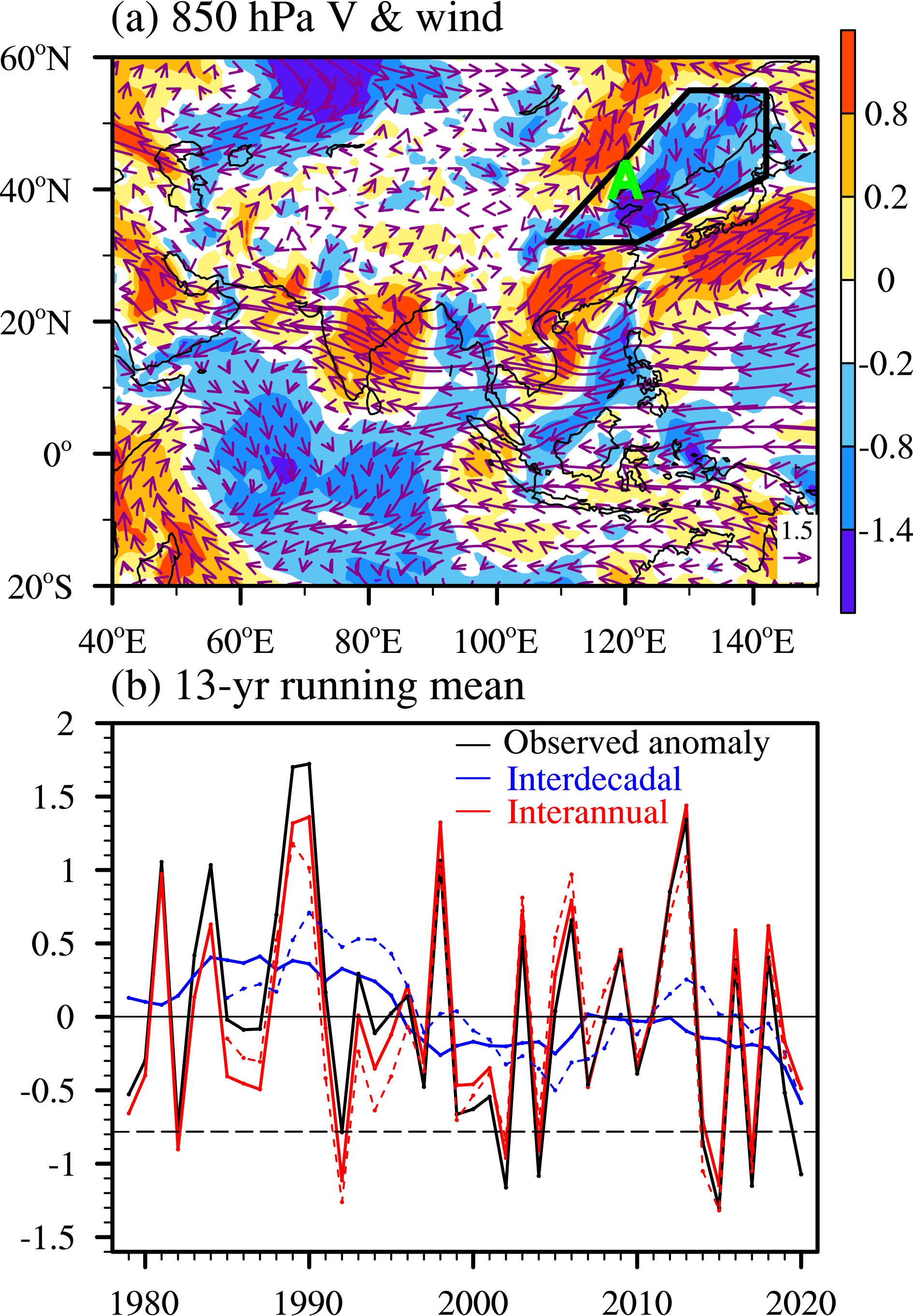 Figure9. (a) The horizontal patterns of 850 hPa wind anomaly field (vector; m s?1) and its meridional wind component (shading; m s?1). Green letter “A” denotes the anomalous anticyclone center over NEA. (b) Time series of the northeasterly wind index (black curve; m s?1) averaged over the black box shown in (a) and its interannual (red lines; m s?1) and interdecadal/trend (blue curve; m s?1) components calculated based on 13-yr running mean with use of Method 1 (solid curve) and Method 2 (dashed curve). A dashed black line denotes negative one standard deviation.
To reveal the relative roles of tropical and midlatitude heat sources in generating the zonally oriented Rossby wave train, we conducted another set of idealized ECHAM4.6 model experiments. Based on the horizontal distributions of precipitation and SST anomalies in JJ 2020 (Fig. 10) and considering the convection in the tropical eastern Pacific could influence the mei-yu rainfall (Zhu and Li, 2016), the positive heating anomaly in the eastern Pacific is selected. Additionally, the observed positive heating in the Indian monsoon region is selected because it could influence the mei-yu onset through a teleconnection pattern (Liu and Ding, 2008) and influence climate in North China via the CGT/SRP patterns (Ding et al., 2011; Chen and Huang, 2012). In addition, the heating in the Atlantic has been proven by many studies to influence precipitation in East Asia through a midlatitude teleconnection pattern (Chen and Huang, 2012; Sun and Wang, 2012; Xu et al., 2015; Han et al., 2018; Lu et al., 2020; Zhu et al., 2020). Therefore, we specified three positive heating regions over the Indian monsoon region (IM; 8o–25oN, 60o–85oE), the tropical Atlantic (TA; 0o–15oN, 60o–10oW), and the eastern Pacific (EP; 5o–15oN, 180o–100oW). In the first experiment (EXP_IM), positive heating resembling the observed precipitation anomaly in the Indian monsoon region was specified. The second experiment (EXP_TA) was forced by the positive heating anomalies in the tropical Atlantic. In the third experiment (EXP_EP), positive heating in the tropical eastern Pacific was specified.
 Figure10. Horizontal distributions of anomalous precipitation (shading; mm d?1) and SST (contour; °C) fields in JJ 2020. Red (blue) contours denote a positive (negative) SSTA. Blue boxes are specified regions for the anomalous heating response experiments.
Figure 11 illustrates the simulated 200 hPa geopotential height and wind responses in the experiments described above. The IM heating induced an upper-level anomalous anticyclone to its northwest as a Rossby wave response (Gill, 1980). The anticyclone perturbed the westerly jet, leading to a wave train pattern as Rossby wave energy propagated downstream, similar to the SRP pattern (Enomoto et al., 2003). As a result, an anomalous anticyclone appeared over NEA (Fig. 11a). The TA heating induced a remote teleconnection in the North Atlantic, presenting a meridional tripole pattern related to the North Atlantic Oscillation (NAO), which further stimulated a Rossby wave train along 45°N, with anticyclonic centers in the North Atlantic, West Asia, and NEA and relatively low pressure centers in between (Fig. 11b). This pattern resembles the summer NAO teleconnection as described in Sun and Wang (2012). The positive heating in the tropical eastern Pacific forced a northeastward Rossby wave train in the Pacific/North America sector and a zonally oriented wave train over the Eurasian Continent (Fig. 11c), similar to the Asia-North America (ANA) pattern (Zhu and Li, 2016).
 Figure11. Simulated geopotential height (contour; m) and wind fields (vector; m s?1) at 200 hPa in response to (a) a positive heating anomaly (shading; °C d?1) over the Indian monsoon region (8°–25°N, 60°–85°E), (b) a positive heating anomaly (shading; °C d?1) over the tropical Atlantic (0°–15°N, 60°–10°W), (c) a positive heating anomaly (shading; °C d?1) in the eastern Pacific (5°–15°N, 180°–100°W). Green boxes are same as those shown in Fig. 8a.
To quantitatively measure the relative contributions of the three heat sources, two geopotential height indices, the NEA index and the wave train (WT) index, were introduced. The NEA index is defined as the geopotential height anomaly averaged over the NEA region (35°–50°N, 115°–135°E), whereas the WT index is defined as the average of the geopotential height anomalies averaged over three observed positive geopotential height anomaly regions (i.e., green boxes in Fig. 8a): (40°–60°N, 60°–15°W), (40°–60°N, 20°–55°E), and (35°–50°N, 115°–135°E). As shown in Fig. 12, the two indices are quite consistent with each other, with a rough estimate of 40%, 25%, and 35% contribution from the forcing in the IM, TA, and EP, respectively, according to the NEA index (WT index). This implies that the midlatitude circulation anomalies, particularly the anomalous anticyclone in NEA, in JJ 2020 were driven by the combined heating anomalies in the IM, EP, and TA.
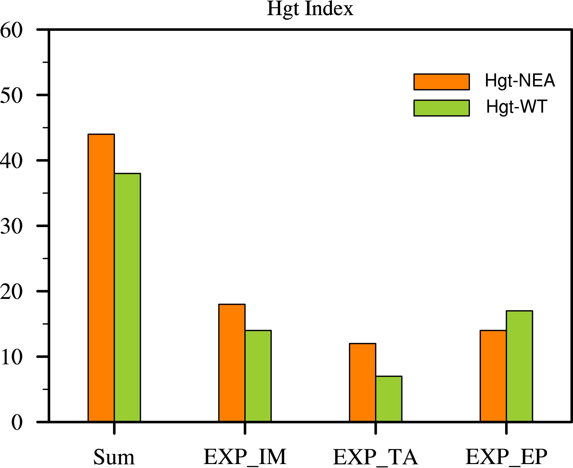 Figure12. The calculated geopotential height indices (m) averaged over the NEA (35°–50°N, 115°–135°E) (orange bar; Hgt-NEA) and along the wave train (green bar; Hgt-WT) for EXP_IM, EXP_TA, EXP_EP, and their summation.
It is found that the exceptionally strong WNPAC in JJ 2020 resulted from the combined impact of a La Ni?a-like SSTA pattern in the equatorial Pacific and an unusal warming in the tropical Indian Ocean. While the composite CP El Ni?o event is characterized by a slow SSTA change in the equatorial central Pacific, the 2019/20 CP El Ni?o was an exception. A quick phase transition happened in early 2020, and by JJ, a cold SSTA appeared in the equatorial Pacific. The cold SSTA induced a negative precipitation anomaly in equatorial CP, which would generate an anomalous anticyclone to its northwest according to the Gill response.
Typically an area of moderate warming appears in the tropical Indian Ocean during the decaying phase of a CP El Ni?o. 2020 again gave us a surprise. Strong IO warming occurred earlier in 2020. The cause of this exceptionally strong IO warming was attributed to the summation of both the interannual and interdecadal/trend components. The strong IO warming induced a Kelvin wave response to its east and maintained the WNPAC through the anticyclonic shear of the Kelvin wave easterly winds (Wu et al., 2010).
The relative roles of the cold SSTA in the Pacific and the warming in the IO in JJ 2020 in contributing to the maintenance of the WNPAC were examined through a set of idealized ECHAM4.6 experiments. The results indicate that the positive heating anomaly in the IO/MC sector contributes about 60%, whereas the negative heating anomaly in the tropical Pacific contributes about 40%. Therefore, both the IO and tropical Pacific SSTAs contributed to the maintenance of the exceptionally strong WNPAC in JJ 2020. Note that the relationship between the diabatic heating and eastern Pacific SST anomalies is not exactly linear (Johnson and Kosaka, 2016), which could lead to different teleconnection patterns. Thus, the anomalous SST-heating relationship needs to be carefully examined in further studies.
It is found that the anomalous northeasterly winds over NEA were part of a zonally oriented Rossby wave train in midlatitude Eurasia. The wave train had a quasi-barotropic vertical structure with alternated anticyclone and cyclone anomalies from the North Atlantic to NEA. The abnormal wind condition in NEA arose from the combined interannual and interdecadal components. One may ask which component is at play for the contribution of the IM, TA, and EP heating in inducing the northeasterly winds, and the regression of the anomalous precipitation (heating) field onto the interdecadal and interannual components of the NWI shows that the interdecadal component of the IM and TA heating plays the dominant role, while the interannual component of EP heating is the main driver.
The relative roles of tropical and midlatitude heat sources in causing the anomalous northeasterlies and the midlatitude wave train were examined through a set of idealized ECHAM4.6 experiments. Three sensitivity experiments with specified heating anomalies in the IM, TA, and EP were carried out. The results confirmed that the anomalous heating in the IM, EP, and TA are important in contributing to the midlatitude circulation anomaly.
The first lesson learned from this 2020 YRV flood event is that one cannot predict El Ni?o impact based on composite maps only. A more detailed tracking of the SSTA evolution, such as slow or quick phase transition, is critical. The second lesson learned is that one needs to consider the impact of the interdecadal/trend component. While the global warming trend amplifies the warming impact in the IO, it would reduce the interannual cold SST anomaly in the same region. The midlatitude circulation anomaly over NEA is a possible impact region by the interdecadal variation. Given that most operational forecast centers around the world use a 30-yr (1981–2010) base line for defining the mean climatology, it is cautious to consider both the impacts of the interannual and interdecadal/trend components for seasonal forecasting.
A limitation of the present study is how to define the interdecadal component at the ending points. In the present study, a non-conventional filtering method was employed to extract the interdecadal component, but errors may arise in estimating the values at the ending points. The method could be improved in future research. Previous studies have suggested that anomalous precipitation in the YRV might be related to the Arctic Oscillation (AO) (He et al., 2017). However, the NWI in the present study has no significant correlation with the AO in both the interannual and interdecadal timescales. A further in-depth study is needed in examining the possible link.
Acknowledgements. This work was jointly supported by China National Key R&D Program 2018YFA0605604, NSFC Grant No. 42088101, NOAA NA18OAR4310298, and NSF AGS-2006553. This is SOEST contribution number 11354, IPRC contribution number 1524, and ESMC number 350.
Open Access This article is distributed under the terms of the Creative Commons Attribution 4.0 International License (
