HTML
--> --> -->An interesting evolution of SSTAs is observed during 2016–18 in the tropical Pacific. Following the 2016–18 consecutive La Ni?a conditions (Feng et al., 2020), a weak El Ni?o event developed during fall of 2018 over the tropical Pacific, which peaked in November 2018, with a maximum positive SSTA of 0.9°C [Based on Extended Reconstructed Sea Surface Temperature version 5 (ERSSTv5) (Huang et al., 2017)]. Subsequently, the positive SSTAs weakened and returned to a neutral condition in June 2019 (Fig. 1a). Historically, as seen from composite analyses after the mature stage, El Ni?o tends to decay rapidly in the next summer and evolves into a La Ni?a-like condition (e.g., Hu et al., 2014). However, a different evolving pattern was seen in the tropical Pacific during 2019. After a short decaying period associated with the 2018/19 El Ni?o condition, the SSTAs intensified yet again in the equatorial Pacific in September 2019 (Fig. 1b). The Ni?o-3.4 index reached the 0.5°C criterion in November 2019, which subsequently persisted for four consecutive overlapping seasons, being very close to the five consecutive overlapping seasons used as a criterion adopted for an El Ni?o event to occur by the Climate Prediction Center (CPC) of the National Oceanic and Atmospheric Administration (NOAA). Therefore, some previous studies simply treated it as a weak Central-Pacific (CP) El Ni?o event (Zheng and Wang, 2021; Zhou et al., 2021). To be consistent with the CPC criterion, here, we treat it as second-year warming in 2019 that occurred following the 2018/19 El Ni?o event. Corresponding atmospheric anomalies are also evident. For example, during June-July 2020, the East Asian plum rain belt suffered from the most severe flooding in decades (e.g., Ding et al., 2021). This extreme plum rain occurred in the background of the decaying stage of the 2018/20 weak El Ni?o event (e.g., Liu and Ding, 2020).
 Figure1. (a) Temporal evolutions of the Ni?o-3.4 index (in °C) for 2019 (red line), the composite year (blue line), and their difference (black line). (b?d) Longitude-time plots of the equatorial Indo-Pacific Ocean SSTAs (in °C) averaged between 5°S and 5°N for (b) 2019, (c) the composite year, and (d) the difference in the SSTAs between 2019 and the composite year.
The reasons for the second-year warming in late 2019 over the tropical Pacific and its triggering mechanism have not been well understood. Previous studies have suggested that ENSO may be affected by processes in the Indian Ocean (Behera and Yamagata, 2003; Saji and Yamagata, 2003). For example, the Indian Ocean Dipole (IOD) is an ocean-atmosphere coupled climatic phenomenon over the tropical Indian Ocean. During a positive IOD, negative SSTAs appear off the Sumatran coast in summer, inducing weaker local convection and easterly wind anomalies. The IOD event can go on to induce worldwide impacts through atmospheric teleconnections and associated interactions with the tropical Pacific Ocean (Behera and Yamagata, 2003; Saji and Yamagata, 2003; Zhang et al., 2021a, b). Previous studies have demonstrated that there are close relationships between the ENSO and IOD (e.g., Annamalai et al., 2005; Izumo et al., 2010). For instance, by using a simple forecast model, Izumo et al. (2010) pointed out that the IOD is an effective predictor of El Ni?o/La Ni?a. Yang and Huang (2021) suggested that the relationship between ENSO and Indian summer monsoon rainfall has been reinforced since 1999-2000, which is linked to the interdecadal transition of ENSO evolution and the associated SSTAs over the tropical Atlantic.
Therefore, the focus of this study is to understand the generation and evolution of the late 2019 second-year warming in the tropical Pacific by addressing the following questions: Which process gives rise to the second-year warming? Did the 2019 super IOD event affect the second-year warming over the equatorial Pacific? What is the underlying feedback mechanism associated with upper ocean dynamics in the tropical Pacific? Understanding the second-year warming in late 2019 and related processes can not only gain new insight into ENSO dynamics, but can potentially provide additional guidance for ENSO prediction. This paper will analyze the basic characteristics and physical mechanisms responsible for the second-year warming in late 2019.
The remainder of this paper is organized as follows. Section 2 describes the data and methods used in the present study. Section 3 analyzes the characteristics of the second-year warming, while section 4 discusses the likely mechanisms responsible for the second-year warming. Section 5 provides a summary and discussion.
2.1. Data
The following observational and reanalysis datasets were used in this work, 1) the monthly 10 m wind velocity and sea level pressure (SLP) fields are from the ERA5 (Copernicus Climate Change Service, 2017), 2) the monthly SST data are from the NOAA ERSSTv5 dataset with a 2° × 2° grid (Huang et al., 2017), and 3) the monthly total downward heat flux, sea surface height (SSH), subsurface temperature, and three dimensional (3D) currents are taken from the GODAS (Behringer and Xue, 2004). Interannual anomalies are departures from the 1980–2020 base period means. The ENSO index is the averaged SSTAs in the Ni?o-3.4 region (5°S–5°N, 120°–170°W). The IOD index (Saji et al., 1999) is the SSTAs difference averaged between (10°S–10°N, 50°–70°E) and (10°S–0°N, 90°–110°E). All the seasonal names used in the present study are relative to the Northern Hemisphere.2
2.2. Methods
Based on the GODAS products, the heat budget in the mixed-layer is diagnosed during the second-year warming after the 2018/19 El Ni?o. The mixed-layer ocean temperature tendency equation can be written as follows (Li et al., 2002; Jin et al., 2003):where


where subscript “sub” denotes the subsurface temperature averaged between 50–100 m.
Following Ren et al. (2013) and ignoring the relatively small terms, the right-hand side of the Eq. (1) are grouped into five linear terms.
in which MC represents the mean current effects on temperature anomalies; ZA is the zonal advection feedback; EK is the Ekman effect; TH is the thermocline feedback; TD is the thermal damping; and Q is the net surface heat flux. A centered finite difference operation is adopted to calculate the mixed-layer heat budget term.
The space-time evolution of El Ni?o events during 1980–2020 is examined by composite analysis. Following the CPC NOAA, an El Ni?o event is defined as a condition when the 3-month running mean of ERSST.v5 SSTAs in the Ni?o-3.4 region meets the threshold of +0.5°C for a minimum of five consecutive overlapping seasons. According to this definition, there were 13 El Ni?o events since 1981 (1982/83, 1986/87, 1987/88, 1991/92, 1994/95, 1997/98, 2002/03, 2004/05, 2006/07, 2009/10, 2014/15, 2015/16, 2018/19). These El Ni?o events are composited (defined as “the composite year”) to construct a space-time evolution, which is compared with that observed in 2019.
3.1. Space-time evolution of the SSTAs
Figure 1a shows the time evolution of Ni?o-3.4 SSTAs in 2019 (red line), the composite year (blue line), and their difference (2019 – composite year, black line). It can be seen that the Ni?o-3.4 index was above +0.5°C at the beginning of 2019, reached its maximum in March, and then decreased slowly during April–July, with a sharp decrease in August. The index kept nearly 0°C in August and September, then increased rapidly in October (about +0.5°C), and remained so by the end of the year. During the composite year, the index was at a maximum in January, then decreased seasonally before entering into a La Ni?a state by the end of the calendar year. From the difference between the SSTAs in 2019 and the composite year, it can be seen that the index in January and February of 2019 was lower than that in the composite year, and the conditions were basically similar to each other in March. However, the evolution is different thereafter in 2019 compared with the composite year. For example, the index in 2019 exceeded the composite case in March, and their difference peaked in July (about 0.5°C). Then the difference decreased in August and September, but increased again in October (about 1°C), and persisted thereafter through the end of the year. One pronounced characteristic in 2019 is the re-emergence of SST warming in autumn, which persisted into March 2020 (not shown). So, obvious differences exist in the SST evolution for 2019 and the composite year.Figures 1b–d show the temporal evolution of SSTAs across the equatorial Indian and Pacific Oceans in 2019, the composite year, and their difference. Most of the equatorial Pacific was occupied by positive SSTAs during the first half of 2019 (Fig. 1b), except for the far-western equatorial Pacific. Beginning in May, positive SSTAs decreased in the eastern equatorial Pacific and transitioned to negative SSTAs in June; this cooling tendency strengthened and spread westward during the following months, and it seemed likely to develop into a La Ni?a condition. However, positive SSTAs persisted in the western-central equatorial Pacific in 2019. Beginning in September, positive SSTAs re-emerged and propagated eastward in the eastern equatorial Pacific; this tendency persisted during the following months, and the second-year warming was evident by late 2019. As for the composite year (Fig. 1c), SSTAs in the central and eastern equatorial Pacific decreased nearly steadily from above-average in the first half of the year to below-average in the latter half of the year, while an out-of-phase SSTA evolution was observed in the far-western equatorial Pacific. The difference between the SSTAs in 2019 and the composite year mainly manifested itself as persistent warming in the west-central equatorial Pacific in May followed by re-intensified warming in the eastern equatorial Pacific in September (Fig. 1d). As for the equatorial Indian Ocean, positive SSTAs emerged in the first half of 2019, while negative SSTAs developed over the eastern equatorial Indian Ocean in May 2019, with the minimum values occurring in October (about –1.0°C). There were weakly positive SSTAs over the equatorial Indian Ocean in the composite year. The difference between SSTAs in 2019 and the composite year mainly manifested itself as the features related to the second-year warming in 2019. We will analyze how the differences over the equatorial Pacific are produced in the following sections.
2
3.2. Characteristics of the subsurface ocean temperature anomalies
To understand the temporal evolution and spatial structures of the second-year warming in the subsurface of the tropical Pacific, the 2-month averaged ocean temperature anomalies along the equator are given in Fig. 2 during 2019 and the composite year.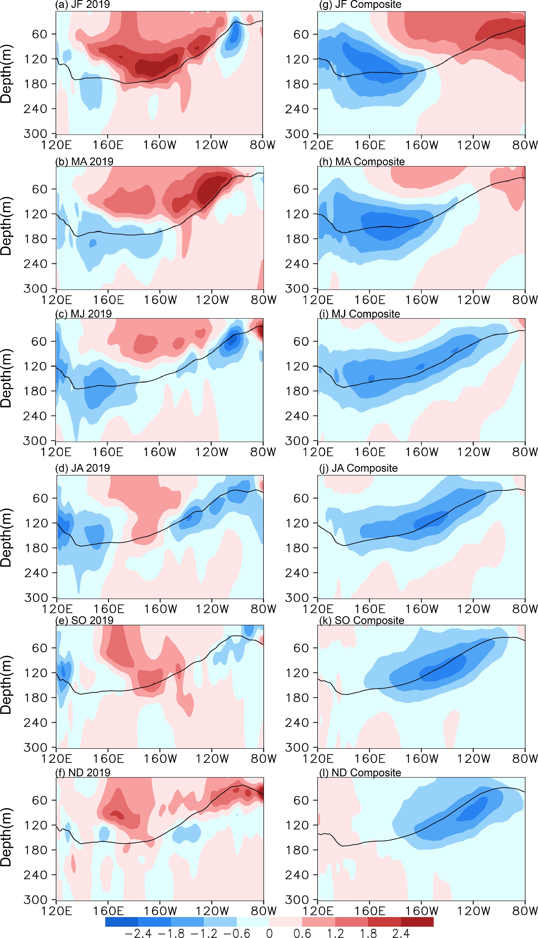 Figure2. Zonal sections of upper ocean temperature anomalies (in °C) in 2019 (left) and the composite year (right) along the equator (averaged over 2°S to 2°N) for (a, g) the January?February mean, (b, h) March?April mean, (c, i) May-June mean, (d, j) July?August mean, (e, k) September?October mean, and (f, l) November?December mean. The black line represents the thermocline depth diagnosed by the 20°C isotherm.
Positive temperature anomalies are seen in most of the equatorial Pacific in January?February 2019 (Fig. 2a), except for a weak negative temperature anomaly that was observed in the far-western equatorial Pacific; at the same time, a pronounced negative temperature anomaly with limited spatial extent was located in the eastern equatorial Pacific. During March?April, negative temperature anomalies in the western equatorial Pacific propagated eastward along the thermocline (Fig. 2b), where they outcropped to the sea surface in May?June (Fig. 2c). This process caused the decay of the positive SSTAs in the eastern equatorial Pacific (Fig. 1b). However, positive ocean temperature anomalies still dominated the western and the central upper layers of the equatorial Pacific. Abnormally warm ocean temperatures stretched downward and broke through the subsurface cold water over the central Pacific in July?August 2019. In the following months, positive temperature anomalies reinforced themselves and expanded, while negative temperature anomalies weakened and retreated to the far-western and far-eastern Pacific in September?October (Fig. 2e). Positive temperature anomalies nearly covered the entire equatorial Pacific in November?December (Fig. 2f), and weak negative temperature anomalies were confined to below 100 meters. Positive subsurface ocean temperature anomalies enhanced and expanded eastward in the eastern equatorial Pacific, outcropped to the sea surface, and produced the second-year warming in late 2019. The evolution in the composite year is very different from that in 2019, in which pronounced negative subsurface ocean temperature anomalies propagated eastward along the thermocline, and positive temperature anomalies diminished in the upper-layer equatorial Pacific (Figs. 2g–i). In the second half of the composite year, negative temperature anomalies strengthened and outcropped to the sea surface, before transitioning into a La Ni?a condition (Figs. 2j–l).
4.1. Triggering processes for the second-year warming
Previous studies have suggested that interocean interactions can trigger or modulate El Ni?o evolution (e.g. Wang et al., 2000; Xie et al., 2009; Ham et al., 2013a, b; Tian et al., 2021). For example, remote effects from the Indian Ocean can modulate ENSO evolution in the tropical Pacific. In particular, a positive IOD event took place in May 2019, which was the strongest event since 1960 (Du et al., 2020; Zhang et al., 2021b). On the intraseasonal timescale, Zhang et al. (2021b) studied the role of the Madden–Julian Oscillation (MJO) as it pertains to Pacific warming. By analyzing daily wind anomalies in 2019, Zhang et al. (2021b) suggested that two MJO events originated from the tropical Indian Ocean and propagated into the western tropical Pacific through 2019, leading to westerly wind bursts which contributed to the development of Pacific warming. Here, we will further examine the influence of the positive IOD event on the second-year warming over the equatorial Pacific in late 2019.Figure 3 gives the time series of IOD indices in 2019 (red bar), the composite year (blue bar), and their difference (solid black line). It can be seen that the IOD event in 2019 occurred in late spring and matured in autumn, which is consistent with the observed development and maintenance of the second-year warming over the equatorial Pacific in 2019. As for the composite year, the IOD indices were nearly zero throughout the year.
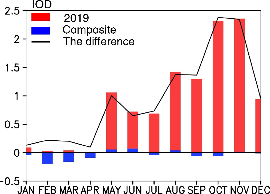 Figure3. Time series of the Indian Ocean Dipole (IOD) index (in °C) in 2019 (red bar), the composite year (blue bar), and their difference (black solid line).
As mentioned earlier, there are two key processes, which are important to the development of the second-year warming in late 2019. One is the persistence of above-average SSTAs over the central equatorial Pacific from May, and the other is the re-intensification of above-average SSTAs over the eastern equatorial Pacific in September.
Figures 4–6 illustrate the spatial distributions of SST, wind stress, and sea level pressure anomalies (SLPAs) over the tropical Indo-Pacific Ocean at some selected periods in 2019 and the composite year. In May 2019, the tropical Pacific was occupied by above-normal SSTAs (Fig. 4a). There were westerly wind anomalies over the western and central tropical Pacific and weak easterly wind anomalies over the eastern tropical Pacific. As for the tropical Indian Ocean, below-normal SSTAs were located in the eastern tropical Indian Ocean, while above-normal SSTAs were located in the western and central tropical Indian Ocean, with the distribution of SSTAs exhibiting an IOD pattern (Fig. 3). Negative SSTAs in the eastern tropical Indian Ocean gave rise to positive SLPAs in the far-western Pacific (Fig. 5a). The positive SLP anomalies expanded eastward to the central tropical Pacific and contributed to the development of anomalous westerlies, which were conducive to the persistence of positive SSTAs in the central equatorial Pacific. As for the composite year (Fig. 6a), the whole tropical Indian Ocean was occupied by weakly positive SSTAs; the eastern tropical Indian Ocean and western tropical Pacific were occupied by weakly positive SLPAs; the anomalous westerly winds over the western and central equatorial Pacific are very weak compared with those in May 2019.
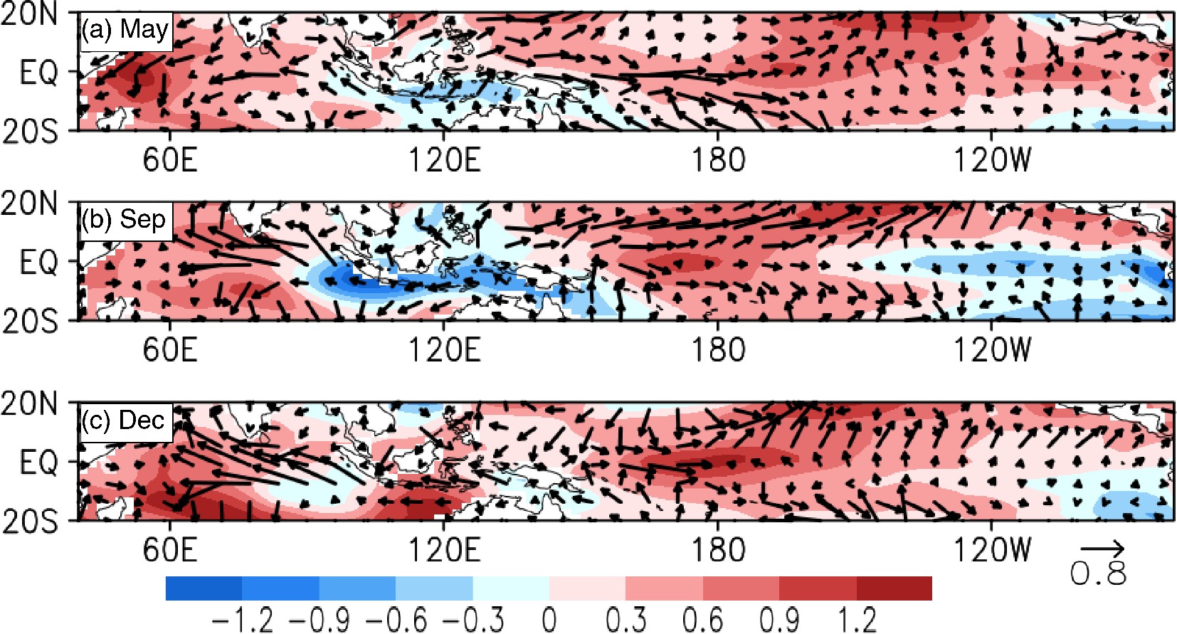 Figure4. Horizontal distributions of SSTAs (shadings; in °C) and wind stress anomalies (vectors; in dyn cm?2; 1 dyn = 10?5 N) for (a) May, (b) September, and (c) December in 2019.
 Figure6. Horizontal distributions of SLPAs (shadings; in hPa), wind stress (vectors; in dyn cm?2), and SSTAs (contours; in °C; positive anomalies in red solid line; negative anomalies in blue dashed line; 0 in black solid line; the interval is 0.3) for (a) May, (b) September, and (c) December in the composite year.
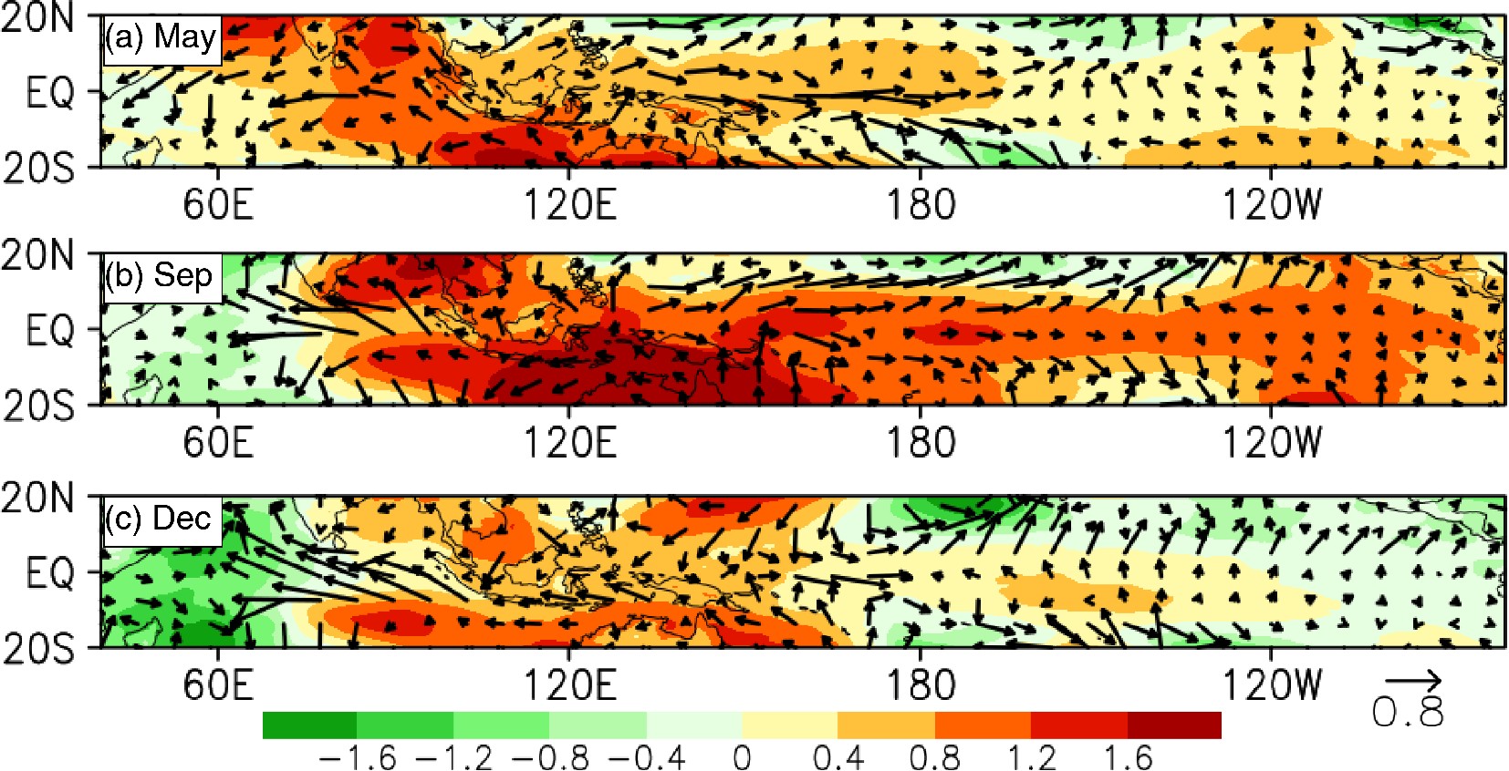 Figure5. Horizontal distributions of SLPAs (shadings; in hPa) and wind stress (vectors; in dyn cm?2) for (a) May, (b) September, and (c) December in 2019.
In September 2019, positive SSTAs were observed in the central tropical Pacific, with its maximum center located near the international date line; but negative SSTAs were seen in the eastern equatorial Pacific (Fig. 4b). According to the Gill Model (Gill, 1980), the corresponding low-level atmospheric responses should consist of westerly wind anomalies to the west of the heating center, and easterly wind anomalies to the east. However, anomalous westerly winds dominated the wide expanse of the western and central tropical Pacific (120°E–140°W), by far exceeding the maximum center of positive SSTAs. Therefore, processes beyond the tropical Pacific warming may have induced the anomalous westerly wind stress. Looking at the Indian Ocean, a strong IOD event was developing at this time, with cold SSTAs covering the eastern tropical Indian Ocean (Fig. 4b). This SSTA pattern generated positive SLP and westerly wind anomalies not only in the eastern tropical Indian Ocean but also in the western tropical Pacific (Fig. 5b), both of which were conducive to the re-intensification of positive SSTAs in the central equatorial Pacific. As for the composite year, weakly positive (negative) SSTAs dominated the tropical Indian Ocean and the western tropical Pacific (the central and eastern equatorial Pacific), which gave rise to weakly positive (negative) SLPAs (Fig. 6b). The distributions of composite SSTAs/SLPAs are very different from those in September 2019, inducing the divergent wind stress anomalies in the central and eastern equatorial Pacific.
At the end of 2019, negative SSTAs over the eastern tropical Indian Ocean and the far-western tropical Pacific separated, noting the presence of strong positive SSTAs along 120°E in the southeastern tropical Indian Ocean sector as well as the southwestern tropical Pacific sector (Fig. 4c). In addition, the SLP anomalies also weakened, and the anomalous westerly winds retreated to the International Date Line (Fig. 5c). At the same time the positive SSTAs dominated the whole equatorial Pacific (centered around the International Date Line), the second-year warming occurred. As for the composite year, negative SSTAs in the central and eastern equatorial Pacific caused positive SLPAs and divergent wind stress anomalies (Fig. 6c), which further strengthened the local negative SSTAs.
2
4.2. The evolution mechanisms for the second-year warming
The atmospheric and oceanic processes responsible for the evolution of the second-year warming in 2019 are examined in detail. Figure 7 shows the temporal evolutions of SST, SLP, zonal wind stress (Taux), and SSH anomalies along the equator of the Indo-Pacific Ocean in 2019. There are coherent relationships among these anomaly fields.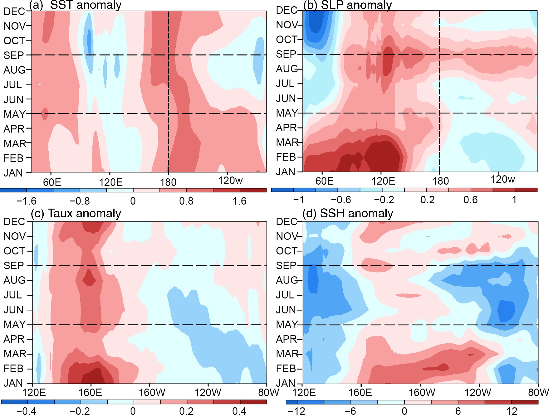 Figure7. Time-longitude cross sections of the equatorial Indo-Pacific Ocean for (a) SSTAs (in °C), (b) sea level pressure anomalies (SLPAs) (in hPa; averaged between 5°S and 5°N) in 2019. Time-longitude cross sections of the equatorial Pacific for (c) Zonal wind stress (Taux) anomalies (in dyn cm?2; averaged between 5°S and 5°N), and (d) SSH anomalies (in mm; along the equator) in 2019.
For the SST field, negative SSTAs were evident over the western equatorial Pacific in early 2019, which gradually expanded westward. In the eastern equatorial Indian Ocean, negative SSTAs developed in May 2019, with the minimum occurring in October (about –1.0°C). Corresponding to these negative SSTAs over the eastern tropical Indian Ocean and the western tropical Pacific, positive SLP anomalies persisted (centered at about 125°E) during 2019, with two maximum centers appearing in late January and August, respectively. At the same time, weakly negative (positive) SLP anomalies also persisted over the central-eastern equatorial Pacific during the first (second) half of 2019. Thus, the corresponding SLP gradient anomalies between the western and central equatorial Pacific were conducive to the development of westerly wind anomalies (Fig. 7c). Indeed, a strong westerly wind stress anomaly (more than 0.4 dyn cm?2) was observed over the western equatorial Pacific (centered around 160°E) in January 2019. This westerly wind anomaly acted to excite a strong dowelling Kelvin wave, which propagated eastward and caused the thermocline to deepen along the equatorial Pacific (Fig. 7d). Subsequently, the intensity of the westerly wind anomaly decreased, accompanying by weakened positive SSH anomalies, which are sustained in the central equatorial Pacific during the spring and summer of 2019. As for the eastern equatorial Pacific, an easterly wind anomaly emerged in early 2019, which propagated westward in the first half of 2019 and exerted an influence on the ocean temperature. On one hand, this easterly wind anomaly increased the upwelling of cold water from the subsurface layer through Ekman pumping and thermocline feedback. On the other hand, this easterly wind anomaly also induced a westward spread of cold water through zonal advection in the eastern Pacific. As a result, positive SSTAs over the eastern equatorial Pacific weakened in the first half of 2019 and transitioned into negative anomalies in summer and autumn. However, the easterly wind anomalies decreased suddenly in July. The relaxation of easterly wind anomalies was conducive to the development of positive SSTAs over the central-eastern equatorial Pacific.
After August, westerly wind anomalies reinforced and expanded eastward to the central equatorial Pacific (around 140°W). Previous studies have demonstrated that westerly wind bursts can trigger an El Ni?o event (e.g., Chen et al., 2015). On one hand, anomalous westerly winds in the western equatorial Pacific excited downwelling Kelvin waves that propagated eastward to the eastern boundary by the end of 2019 (Fig. 7d). The strong subsurface warming which resulted from downwelling Kelvin waves quickly reversed the negative SSTAs to be positive. On the other hand, anomalous westerly winds led to surface warming through zonal advection. The warming surface condition in the western equatorial Pacific expanded eastward, while the cold SST anomalies in the eastern equatorial Pacific decreased rapidly in October (Fig. 7a). These processes persisted during late 2019, then positive SSTAs dominated the whole equatorial Pacific and the second-year warming occurred.
To further examine the spatial characteristics of the Kelvin wave excited by anomalous westerly winds in detail, the spatial structure of SSH anomalies was given in Fig. 8. Beginning in September, driven by the strengthening of the anomalous westerly winds (Fig. 7c), a positive SSH anomaly in the central equatorial Pacific extended eastward (Fig. 8a), and then propagated throughout the central-eastern equatorial Pacific, which is seen as a fluctuating wave signal (Fig. 8b). Negative SSH anomalies over the eastern equatorial Pacific were divided into two parts, located on either side of the equator. In November, positive SSH anomalies reached the eastern equatorial Pacific, and the negative SSH anomalies over the eastern equatorial Pacific noticeably weakened (Fig. 8c). In December, driven by the reintensified anomalous westerlies, positive SSH anomalies expanded eastward again from the central equatorial Pacific (Fig. 8d). These processes contributed to the second-year warming in late 2019.
 Figure8. Horizontal distributions of sea surface height (SSH) anomalies (shadings; in mm) for (a) September, (b) October, (c) November, and (d) December in 2019.
Previous studies have shown that the effects of the anomalous eastward advection and the variation in the thermocline are the main reasons for the development of El Ni?o (An and Jin, 2001). Ashok et al. (2007) pointed out that the equatorial thermocline feedback plays a key role in the evolution of the ENSO in the Eastern-Pacific (EP) ENSO’s evolutions, whereas the zonal advection plays an important role in the the Central-Pacific (CP) ENSO’s evolutions (e.g., Kug et al., 2009; Marathe et al., 2015). In order to quantify the specific contributions attributed to each physical process to the second-year warming in late 2019, the SST equation was used to diagnose the mixed-layer heat budget. Figure 9 illustrates the evolution of each physical process over time. From the sum of all terms in 2019 (Fig. 9f), it can be seen that the cooling effect was mainly located in the eastern equatorial Pacific (120°–80°W), while the warming effect was located in the western and central equatorial Pacific, with two maximum centers (exceeding 1°C month?1) emerging in early 2019 and mid-late 2019, respectively. As a whole, the zonal advection feedback (Fig. 9a), the thermocline feedback (Fig. 9b), and Ekman pumping (Fig. 9d) contributed to the warming of the mixed-layer temperature in the western and central equatorial Pacific, but cooling effects in the eastern equatorial Pacific. In terms of the roles of mean ocean currents (Fig. 9c) and thermal damping (Fig. 9e), they provided a cooling effect on the mixed-layer temperature variation in the western and central equatorial Pacific, but a warming effect in the eastern equatorial Pacific. To sum up, the SST warming in the fall of 2019, corresponding to the second-year warming, was mainly induced by the zonal advection feedback and thermocline feedback. The zonal advection feedback played a major role over the central-eastern equatorial Pacific during August-November (about 0.7°C month?1), while the thermocline feedback played a major role in December (about 0.4°C month?1).
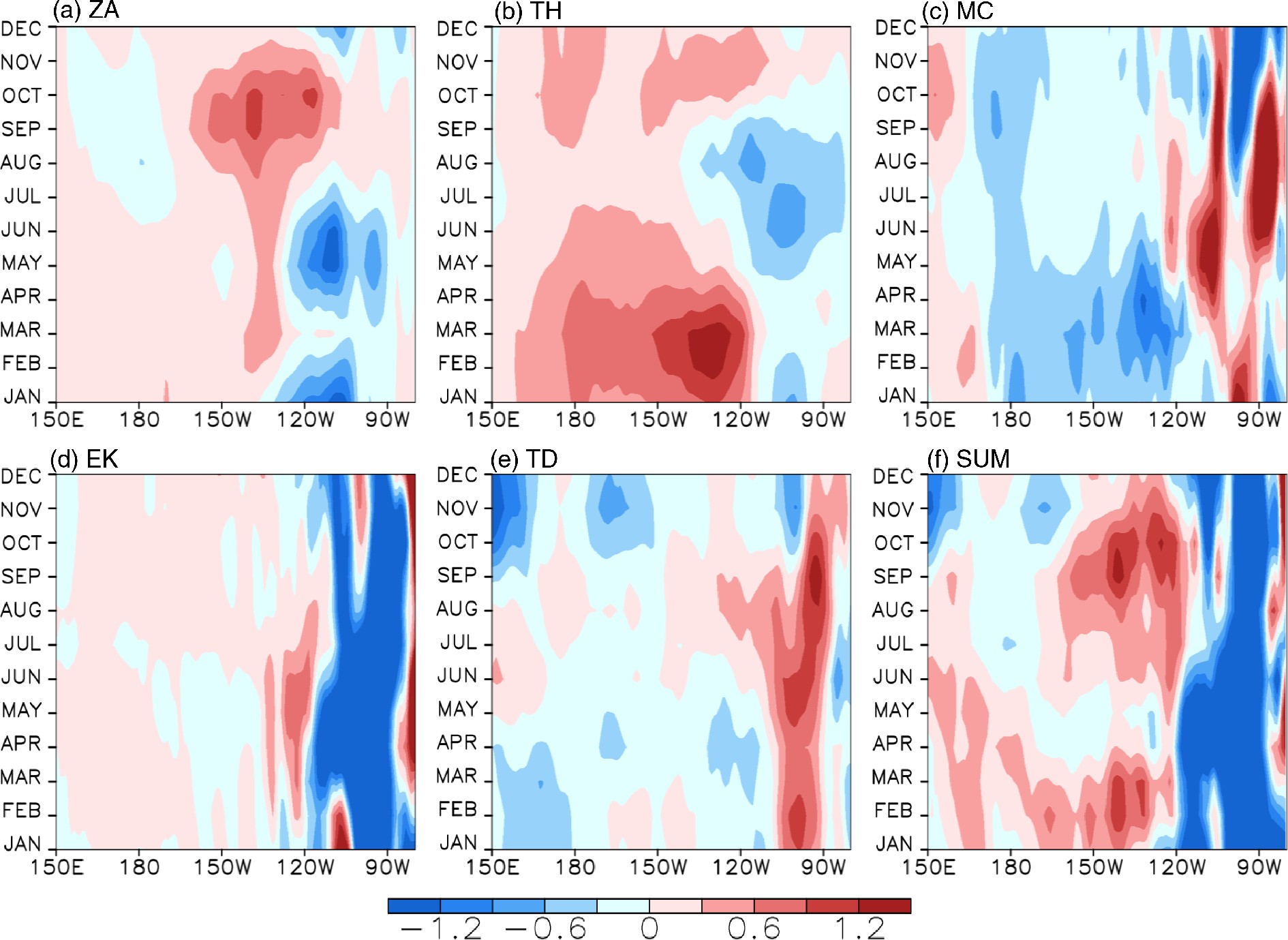 Figure9. Temporal evolutions of the mixed-layer dynamical and thermodynamical terms (in °C month?1) along the equator (averaged between 2°S and 2°N) in 2019 for (a) ZA, (b) TH, (c) MC, (d) EK, (e) TD, and (f) SUM. Here, ZA represents zonal advection; TH represents thermocline feedback; MC represents mean current effect; EK represents Ekman effect; TD represents thermal damping, and SUM= ZA+TH+MC+EK+TD.
This study suggested that an exceptionally strong positive IOD event played a critical role in remotely triggering the 2019 second-year warming in the tropical Pacific (Fig. 7). Associated with the development of the positive IOD event, negative SSTAs in the eastern tropical Indian Ocean gave rise to positive SLP anomalies over wide expanses of the eastern tropical Indian Ocean and the western tropical Pacific in mid-late 2019. The SLP gradient anomalies between the western and central equatorial Pacific contributed to the intensification of anomalous westerly winds over the western equatorial Pacific. These conditions were conducive to the development of the second-year warming in late 2019.
The related evolution processes and effects were summarized as follows (see Fig. 10). In the first half of 2019, most of the tropical Pacific was occupied by positive SSTAs. Beginning in May, negative subsurface ocean temperature anomalies propagated to the eastern equatorial Pacific, where they outcropped to the surface, which cooled down the sea surface. Typically, this sequence foretells that a La Ni?a condition is on the way, just like that transpired in the composite year. However, an extremely positive IOD event emerged and gave rise to positive SLPAs over the eastern tropical Indian Ocean and the western tropical Pacific. The SLPA gradient between the western and central tropical Pacific was conducive to the re-intensification and persistence of anomalous westerly winds in the western and central tropical Pacific. These conditions were favorable for generating warmer SSTs in the western equatorial Pacific. At the same time, subsurface warm water was sustained in the western and central equatorial Pacific, which served to further maintain the above-normal SSTAs. From late August, the westerly wind anomalies expanded eastward, which caused the SST warming in the eastern equatorial Pacific through zonal advection. Simultaneously, the westerly wind anomalies excited downwelling Kelvin waves in the western basin, which propagated eastward and warmed the SST in the eastern equatorial Pacific due to the deepening of the thermocline. Thus, both the anomalous westerly winds and anomalous subsurface warm water contributed to the second-year warming in late 2019. Mixed-layer heat budget analyses indicate that the zonal advection feedback played a major role over the central and eastern equatorial Pacific during August–November (about 0.7°C month?1), while the thermocline feedback played a major role in December (about 0.4°C month?1).
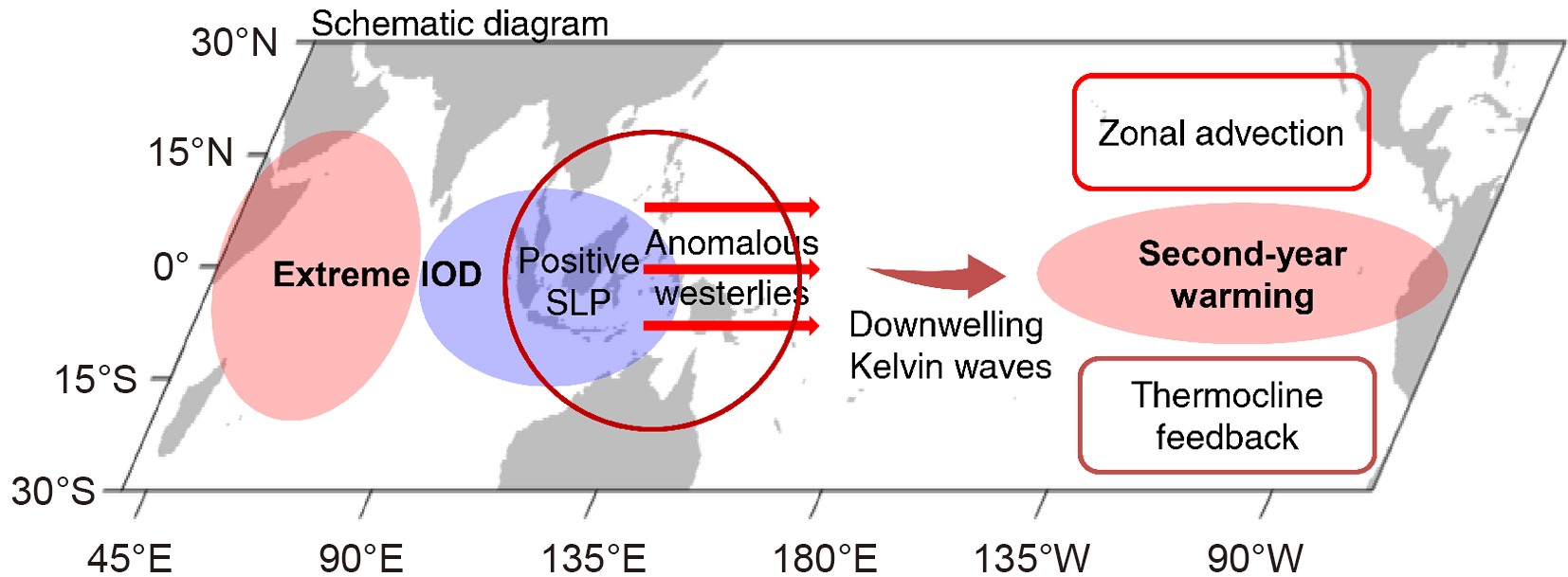 Figure10. Schematic diagram showing the pathway by which an extreme IOD event triggers the late 2019 second-year warming in the eastern equatorial Pacific.
Besides the 2019/20 second-year warming, two other second-year warming (1987/88 and 2015/16 events) occurred during the analysis period. We checked the IOD index for these episodes and found that both the IOD indices were positive. However, the positive index in 1987 was ~0.4°C, which failed to reach the IOD event criterion of ~0.6°C. In contrast, the IOD index in 2015 did meet the criterion and had a maximum of ~0.9°C. The 1987/88 event has been studied by Chen and Li (2018), who suggested that the equatorial westerly wind anomalies, south of the western North Pacific cyclone, triggered downwelling Kelvin waves, prolonging the positive SSTAs throughout 1987. As for the 2015/16 super El Ni?o event, it attracted great attention and interest from researchers. Westerly wind bursts (Lian et al., 2017; Xue and Kumar, 2017; Hu and Fedorov, 2019) and the local effects of the above-normal subsurface heat content (Zhang and Gao, 2017) were considered to be the main processes responsible for the 2015/16 second-year warming. Besides, Kim and Yu (2020) studied the multi-year El Ni?o events in a 2 200-yr simulation of the Community Earth System Model (version 1) and found that the phase information of the preceding winter North Pacific Oscillation and fall IOD together can be used to project the evolution characteristics of El Ni?o events. Tokinaga et al. (2019) investigated the fragile relationship between ENSO and the Atlantic Ni?o by comparing the influence of multi-year and single-year ENSO events over the past 113 years and found that the ocean-atmosphere coupling in the equatorial western-to-central Pacific plays a major role in shaping ENSO teleconnections in boreal spring. The generation mechanism and global impacts of a multi-year El Ni?o event need further studies.
Global warming caused by human activities has led to the increase and intensification of extreme climate events, which have a serious impact on the sustainable development of human society and people's lives and property. Under the scenario of high greenhouse gas emissions, the frequency of extreme positive IOD events can increase in most climate models (Cai et al., 2014). Thus, focused studies on the relationship between extreme IOD and El Ni?o events are of great significance and have the potential to improve short-term climate prediction. Further investigation is therefore needed and will be performed.
Acknowledgements. We appreciate the constructive comments from three reviewers. This work is jointly supported by grants from the National Key Research and Development Program (Grant No. 2018YFC1505802), the National Natural Science Foundation of China (Grant Nos. 41576029; 42030410; 41690122(41690120); 41420104002), and the Strategic Priority Research Program of Chinese Academy of Sciences (Grant Nos. XDA19060102, XDB 40000000 and XDB 42000000).
