Yuanyuan YANG^1,2,
Min ZHONG^1,2,3,
Wei FENG^1,3,,,
Dapeng MU⁴

Corresponding author: Wei FENG,fengw28@mail.sysu.edu.cn;

1.State Key Laboratory of Geodesy and Earth’s Dynamics, Institute of Geodesy and Geophysics, Innovation Academy for Precision Measurement Science and Technology, Chinese Academy of Sciences, Wuhan 430077, China
2.University of the Chinese Academy of Sciences, Beijing 100049, China
3.School of Geospatial Engineering and Science, Sun Yat-sen University, Zhuhai 519082, China
4.Institute of Space Sciences, Shandong University, Weihai 264209, China
Manuscript received: 2021-01-27
Manuscript revised: 2021-04-24
Manuscript accepted: 2021-05-19
Abstract:The deep ocean below 2000 m is a large water body with the sparsest data coverage, challenging the closure of the sea-level budget and the estimation of the Earth’s energy imbalance. Whether the deep ocean below 2000 m is warming globally has been debated in the recent decade. However, as the regional signals are generally larger than the global average, it is intriguing to investigate the regional temperature changes. Here, we adopt an indirect method that combines altimetry, GRACE, and Argo data to examine the global and regional deep ocean temperature changes below 2000 m. The consistency between high-quality conductivity-temperature-depth (CTD) data from repeated hydrographic sections and our results confirms the validity of the indirect method. We find that the deep oceans are warming in the Middle East Indian Ocean, the subtropical North and Southwest Pacific, and the Northeast Atlantic, but cooling in the Northwest Atlantic and Southern oceans from 2005 to 2015.
Keywords: deep ocean warming,
GRACE,
Argo,
GO-SHIP,
altimetry
摘要:近几十年来，海洋加速变暖对地球气候系统和人类生活已经产生了重大影响。由于深海直接观测资料的不足，人类对于海洋冷暖的认识一般局限于海洋上层2000 m。海洋吸收的多余热量是否传递到了深海，一直是全球变化领域最具挑战性的科学问题之一。本文结合卫星测高、卫星重力和海洋温盐数据间接的研究了全球和区域深海冷暖变化，发现了2005-15年印度洋中东部、亚热带西南太平洋和东北大西洋深海变暖，而西北大西洋和南大洋深海变冷，并利用全球海洋船载水文调查计划(GO-SHIP)的深海温盐观测数据验证了研究结果的可靠性。由于这两种方法的时空分辨率存在较大差异，间接估算的区域比容趋势值均大于GO-SHIP的CTD的观测结果。因此，间接法可用于定性地探测深海冷暖变化，但仍难以准确量化深海的温度和热含量变化。
关键词:深海变暖,
GRACE,
Argo,
GO-SHIP,
卫星测高

HTML

--> --> -->

The ocean has absorbed more than 90% of the excess heat which has accumulated in the climate system caused by greenhouse gases since the 1970s and has contributed about 40% to global sea-level rise since the 1990s (IPCC, 2013). Thus, the ocean heat content (OHC) change and steric sea-level change are vital climate metrics. Recent estimates of OHC and associated steric sea-level rise based on observational records and models indicate that ocean warming is significant in the past half-century and the warming is accelerating in recent decades (Durack et al., 2018; Cheng et al., 2019, 2020). However, these estimates are limited to the upper 2000 m of the ocean, mainly due to the lack of sufficient temperature observations in the deep ocean below 2000 m. Whether the deep ocean below 2000 m is warming has been a matter of great controversy (Meyssignac et al., 2019). The deep ocean mentioned in this study refers to the ocean below 2000 m, exceeding the current maximum sampling range of the Argo floats.
Both the international World Ocean Circulation Experiment (WOCE) and the Hydrographic Programme and Global Ocean Ship-based Hydrographic Investigations Program (GO-SHIP) have offered direct and high-quality measurements (including temperature, salinity, etc.) to monitor the deep ocean changes based on repeated hydrographic sections (Desbruyères et al., 2016, 2017). However, it is still a challenge to produce a time series for the deep ocean changes, instead, only a long-term trend estimate is provided (e.g., Purkey and Johnson, 2010; Desbruyères et al., 2014; Talley et al., 2015). In addition to the in situ observations, there are many model or reanalysis products available, but these data suffer from model bias or strength of the observation constraint, therefore, the process by which the deep ocean changes is still debatable (Song and Colberg, 2011; Palmer et al., 2017; Garry et al., 2019).
At the beginning of this century, the emergence of the Gravity Recovery and Climate Experiment (GRACE) satellites, altimetry satellites, along with in situ Argo floats has provided a completely new perspective to study deep ocean warming (Purkey et al., 2014; Volkov et al., 2017). Theoretically, one can deduce the barystatic sea-level change (GRACE-derived) and steric sea-level change of the upper 2000 m depth (Argo-derived) from the total sea-level change (altimeter-derived), and estimate the steric contribution from the deep ocean, which is an affirmative indicator of ocean warming (Llovel et al., 2014; Chen et al., 2018; Asbj?rnsen et al., 2019; Chang et al., 2019; Royston et al., 2020). Previous studies found that the global sea-level budget (SLB) based on altimetry, GRACE, and Argo (0–2000 m) appears to be closed within uncertainty over various time scales, and the remaining part (the deep ocean under 2000 m) contributes almost zero with great uncertainty (Llovel et al., 2014; Dieng et al., 2015; Kleinherenbrink et al., 2016; Volkov et al., 2017; WCRP Global Sea Level Budget Group, 2018; Frederikse et al., 2020; Royston et al., 2020). This indicates that the deep ocean changes below 2000 m are currently still too small to be detectable from data uncertainty using the current Earth Observation System.
However, regional changes are always larger than global averages, where the signals tend to cancel out, it is desirable to estimate regional changes based on altimetry, GRACE, and Argo data. In this study, we estimate the regional pattern of deep steric sea-level (DSSL) change from 2005 to 2015 by using an indirect method with multiple datasets of altimetry, GRACE, and Argo, i.e. “Alt.–Argo–GRACE”. We then assume that the DSSL changes are mainly due to temperature changes rather than salinity. Consequently, the pattern of global temperature in the deep ocean can be obtained. This conceptual pattern has garnered great interest in the community as it highlights the “hot spots” or “cold spots”, which are important to the deep ocean heat uptake. This regional pattern could also guide the deployment of Deep-Argo floats.
As indicated before, our study relies on a basic assumption that the DSSL change is dominated by the temperature change. This assumption is valid in most of the global regions except for the birthplace of deep-water mass, such as the subpolar region of the North Atlantic and Southern Oceans (Stammer et al., 2013). Therefore, the location where the DSSL changes drastically is probably a good indicator of the deep ocean temperature changes. To test this assumption, we have compared our results with direct hydrographical measurements from GO-SHIP and such a comparison supported this assumption.
In addition, recent investigations found a significant signal of long-term accelerated deep-ocean warming in the subtropical South Pacific Basin based on GO-SHIP and pilot Deep-Argo floats from 2005 to 2018 (Johnson and Doney, 2006; Volkov et al., 2017; Johnson et al., 2019; Purkey et al., 2019), which is also confirmed by our indirect method.
This paper is structured as follows. Section 2 introduces the data and methodology used in this study. Section 3 presents the spatial-temporal variability of the deep ocean steric sea-level change and the verification results. Section 4 provides a main discussion and summary.

To derive the deep ocean steric sea-level changes, estimate their uncertainty, and verify the results, four datasets are used: satellite altimetry, satellite gravity, Argo, and GO-SHIP CTD data (the detailed information is provided in Table 1).

Data Type	Institution/Datasets	Reference or website
Altimetry	AVISO	https://www.aviso.altimetry.fr/
	CSIRO	http://www.cmar.csiro.au/sealevel/sl_data_cmar.html
	CMEMS	https://marine.copernicus.eu/
Argo	BOA	(Li et al., 2017)
	CORA	(Cabanes et al., 2013)
	EN4_g10	(Gouretski and Reseghetti, 2010; Good et al., 2013)
	EN4_l09	(Levitus et al., 2009; Good et al., 2013)
	IAP	(Cheng et al., 2017)
	IPRC	http://apdrc.soest.hawaii.edu/
	ISAS15	(Gaillard et al., 2016)
	JAMSTEC	(Hosoda et al., 2010)
	NCEI	(Levitus et al., 2012)
	SIO	(Roemmich and Gilson, 2009)
GRACE	CSR RL06	http://podaac.jpl.nasa.gov/grace/
	JPL RL06	http://podaac.jpl.nasa.gov/grace/
	GFZ RL06	http://podaac.jpl.nasa.gov/grace/
	ITSG-Grace2018	(Kvas et al., 2019)
	JPL-M RL06	(Wiese et al., 2016)
	CSR-M RL06	(Save et al., 2016)
CTD	GO-SHIP	https://cchdo.ucsd.edu/
	WOCE	https://cchdo.ucsd.edu/

Table1. Summary of satellite and in situ datasets used in this study from 2005 to 2015.


Three monthly sea surface height (SSH) grid products derived from a series of satellite altimeter missions are released by the Archiving, Validation, and Interpretation of Satellite Oceanographic (AVISO), the Copernicus Marine Environment Monitoring Service (CMEMS), and the Commonwealth Scientific and Industrial Research Organisation (CSIRO) covering the period from 1993 to present. We remove glacial isostatic adjustment (GIA) effect correction on long-term ocean bottom deformation (Roy and Peltier, 2015, 2017) and elastic loading ocean bottom deformation (OBD) correction using GRACE data (García et al., 2006; Vishwakarma et al., 2020) before joint calculation.
Ten monthly temperature and salinity datasets used to calculate steric sea-level change from the sea surface to a depth of 2000 m (${\rm{SS}}{{\rm{L}}_{2000}}$) (Jayne et al., 2003) are retrieved from the following institutions: the Second Institute of Oceanography, Ministry of Natural Resources, China (BOA), the Coriolis Ocean database for ReAnalysis (CORA), France, the UK Met Office (EN4), the Institute of Atmospheric Physics, Chinese Academy of Sciences, China (IAP), the International Pacific Research Center (IPRC) at the University of Hawaii, USA, the Laboratory for Ocean Physics and Satellite remote sensing (ISAS15), France, the Japan Agency for Marine-Earth Science and Technology (JAMSTEC), the National Centers for Environmental Information (NCEI), USA, and the Scripps Institution of Oceanography (SIO) at the University of California San Diego, USA. These datasets are mainly derived from Argo floats that have been deployed since 1999 and achieved near-global coverage since 2005 (Jayne et al., 2017). Some of these products also merge Argo data with other instrumental data such as CTD, Mooring, XBTs, Glider, etc., hereafter, referred to simply as Argo. The steric sea-level change was calculated based on temperature, salinity, and density of seawater using the Thermodynamic Equation of Seawater-2010 (TEOS-10).
Four, monthly GRACE fully normalized spherical harmonic coefficient products from 2002–17 are respectively provided by four data processing centers: the Center for Space Research (CSR) of the University of Texas at Austin, the German Research Centre for Geosciences (GFZ), the Jet Propulsion Laboratory (JPL), and the Institute of Geodesy at Graz University of Technology (ITSG). To obtain the ocean mass chang in SSH (${\rm{SS}}{{\rm{H}}_{{\rm{mass}}}}$), we carry out a series of standard post-processing routines, including C20 coefficients replacement by the solutions from Satellite Laser Ranging (Cheng and Ries, 2017), adding back degree-1 coefficients (Swenson et al., 2008; Sun et al., 2016) and GAD product, removing global mean atmospheric pressure changes (Uebbing et al., 2019), GIA corrections based on the ICE6G-D model (Peltier et al., 2018), and by applying a 300 km Gaussian smoothing (Johnson and Chambers, 2013). Moreover, GRACE RL06 mascon grid solutions from CSR and JPL with all corrections applied are also used (named CSR-M, and JPL-M, respectively).
Due to the different spatial and temporal resolution of each product, we perform the necessary linear interpolation processing to standardize the data into 1° × 1°grids in both longitudinal and latitudinal directions, which has a negligible impact on the linear trend of the DSSL changes according to some tests (not shown).
in which, SSH represents the total sea surface height changes from altimetry, SSL₂₀₀₀ represents steric sea-level changes to a depth of 2000 m from Argo, and SSH_mass represents the ocean mass changes from GRACE.
The high precision full-depth temperature and salinity hydrographic measurements obtained by ship-based CTDs are shared by CLIVAR and Carbon Hydrographic Data Office (CCHDO). Figure 1 shows the location and sample numbers of repeated sections during the whole period of the GRACE era. The repeated sections we define require that multiple CTD records (not necessarily from the single sections) fall within the same 1° grid point. In Fig. 1, we can find that about 80% of the repeated sections have only two occupations over 15 years. We follow the interpolation method in (Purkey and Johnson, 2010) to calculate the temperature and salinity change along the GO-SHIP sections, and then apply the formulas (12)–(18) found in Jayne et al. (2003) to calculate the DSSL change. During the calculation, we use the World Ocean Atlas 2018 (WOA18) as a climatological mean-field for both temperature and salinity.
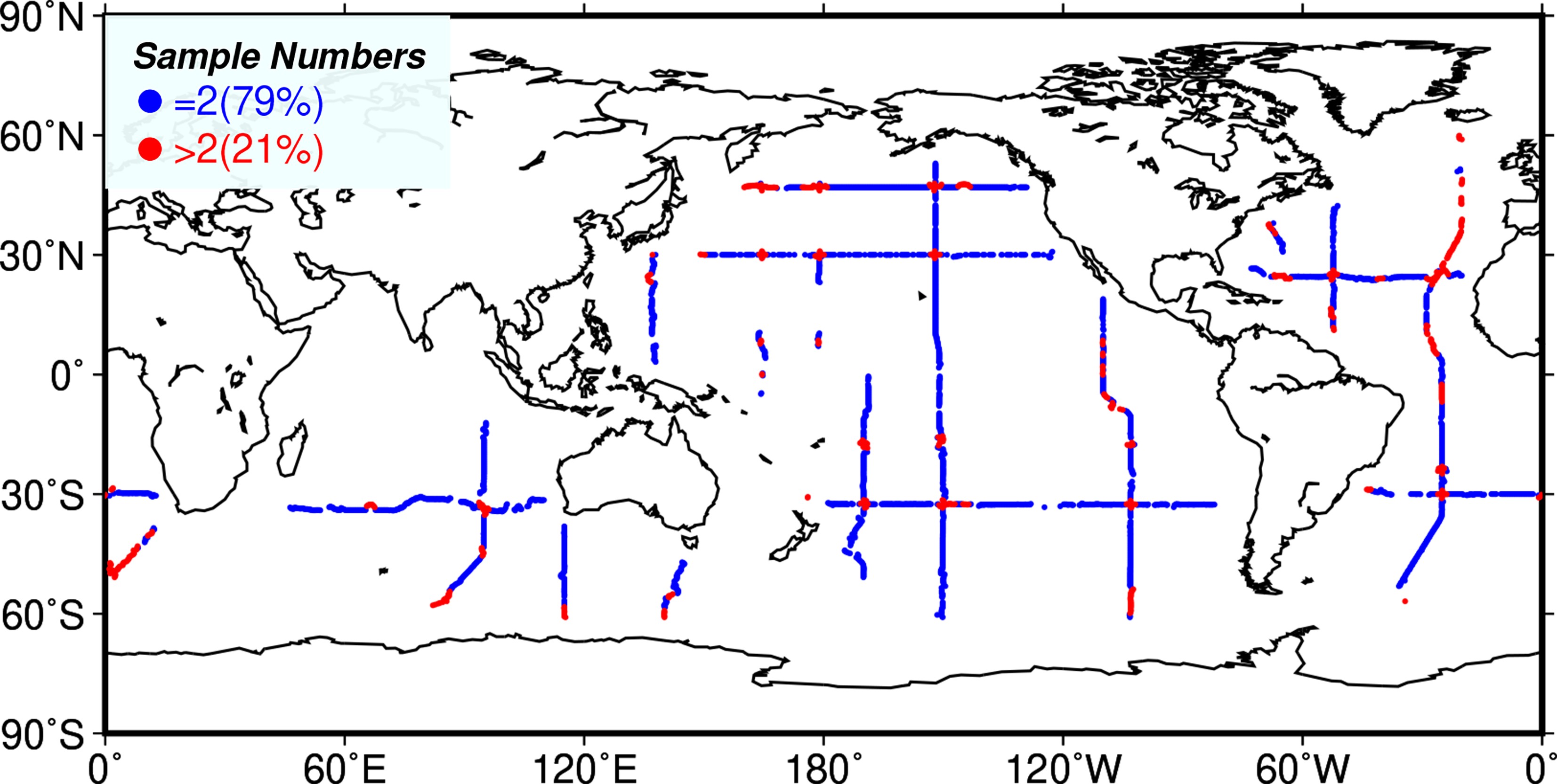Figure1. Locations of repeated oceanographic sections during the GRACE era (2002.4–2017.6). The blue symbols indicate only two occupations of each section during the time period, while red symbols indicate more than two occupations. The percentages in the legend represent the proportions of corresponding sample numbers.


We adopted a reasonable assumption that the deep steric change is dominated by temperature change. We are then able to calculate the responding deep ocean heat content change derived from indirect deep steric change. The conversion coefficient of these two physical quantities is obtained by the following steps. First, we calculated both the corresponding thermal expansion coefficient and density based on the WOA18 temperature and salt field data. Then, the conversion factor is calculated according to the formula in the previous literature (Purkey and Johnson, 2010). Meyssignac et al. (2019) had discussed the global OHC obtained by different coefficients. However, these coefficients do not make a significant difference in the spatial distribution of OHC changes (Purkey and Johnson, 2010). Since the conversion coefficient fluctuates around 1.0, the spatial pattern of deep steric change is similar to the mapped heat content change.
All of the products are combined together to provide a super ensemble. The ensemble mean is our final estimate and the uncertainty is calculated by the standard deviation of the ensemble members (Fig. 2). This uncertainty estimation assumes a “Gaussian” distribution of the error and neglects any common systematic biases. This technique has been widely used because there is no clear indication of large systematic errors in the current datasets. For GRACE, we also considered the uncertainty associated with different GRACE processing parameters (Landerer et al., 2020).
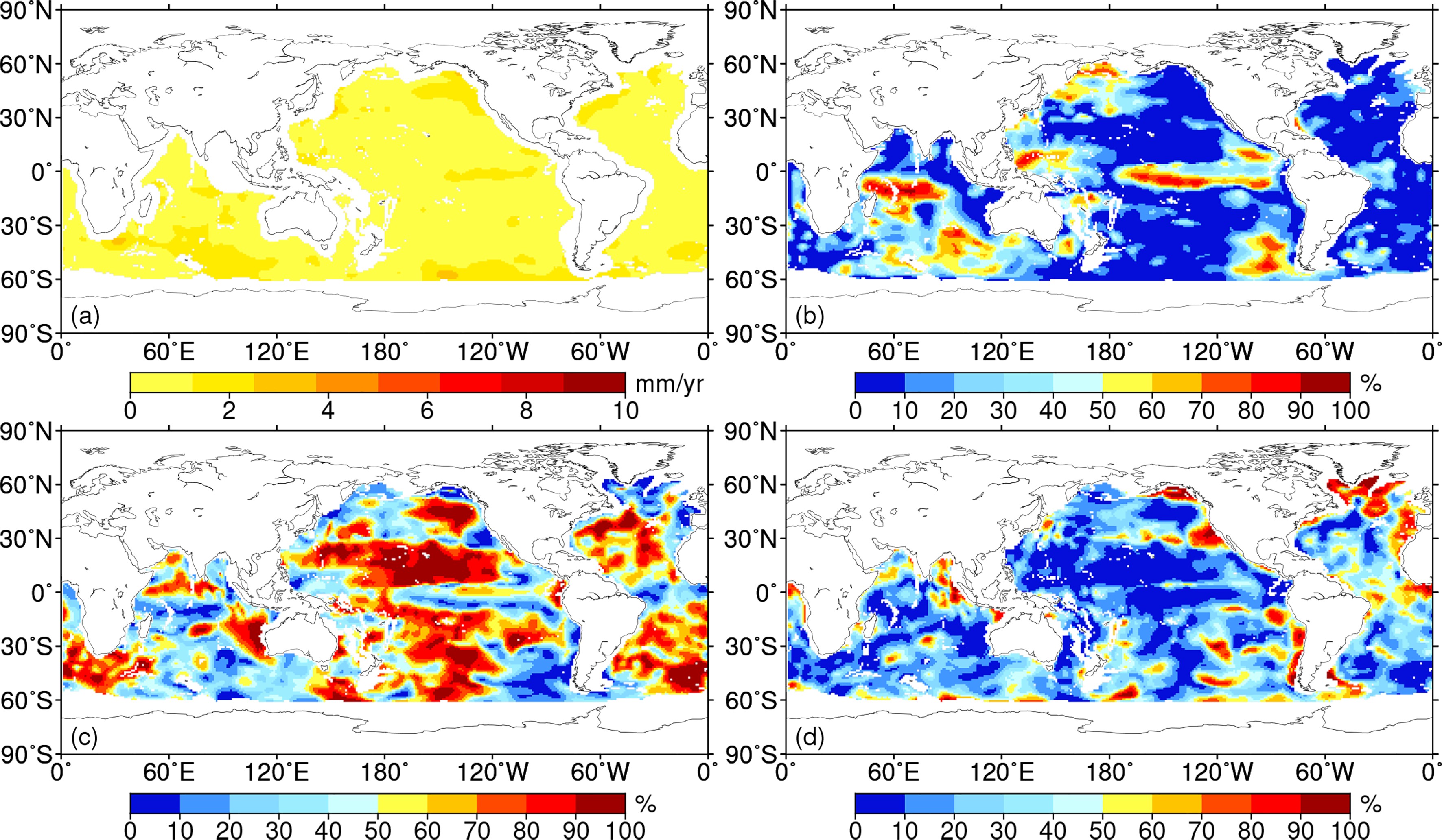Figure2. The standard deviation of (a) the linear trend of ${\rm{DSSL}}$ and the relative contribution of (b) total sea-level change from altimetry, (c) steric sea-level change (0–2000 m) from Argo, and (d) GRACE-based ocean mass change in the indirect method over the period 2005–15 based on the corresponding datasets listed in Table 2. The percentages of the variance explained in (b–d) are derived from the variance of each component divided by the total variance.


Hydrological data are used for verification. Due to the sparse sampling of hydrological sections, we prefer to use the trend spread of different sections in the region as its uncertainty estimate of the regional trend. Ship-based repeated hydrological sections are currently recognized as high-quality data that can be used to validate the DSSL change and separate the contributions of temperature and salinity. However, due to the sparse spatial and temporal sampling of ship-based observations, they are only used to validate the sign of the derived DSSL change by “Alt.–Argo–GRACE”.
This study focuses on the period from January 2005 to December 2015, because the Argo network has near-global ocean coverage since 2005, and the accuracy of GRACE data is significantly reduced since June 2016 mainly because of the great change of the satellite operations status (Landerer et al., 2020). Furthermore, considering the difference in the spatial coverage of the datasets, as well as the inevitably affected by leakage errors and seismic deformation effects, we only consider the open ocean regions with 500 km buffer from the coastline and mask out the regions affected by the large earthquakes, i.e., the 2004 Sumatra-Andaman earthquake, the 2010 Maule earthquake, and the 2011 Tohoku-Oki earthquake (Han et al., 2006, 2010, 2011). The same 300 km Gaussian smoothing has been applied to altimetry data and Argo data to maintain the same resolution with GRACE data.

2

-->

3.1. Global and regional DSSL change

Figure 3 shows the global mean time series of ${\rm{SSH}}$, ${\rm{SS}}{{\rm{L}}_{2000}}$, ${\rm{SS}}{{\rm{H}}_{{\rm{mass}}}}$, and ${\rm{DSSL}}$ based on the combination of currently available datasets within a two standard deviation uncertainty range. During 2005–15, the steric sea-level change accounts for ~1/3 of global sea-level rise, and most of the steric contribution comes from the ocean above 2000 m (Fig. 3). The linear rate of the DSSL change is 0.07±0.18 mm yr^?1 from the residuals of “Alt.–Argo–GRACE” from 2005 to 2015, which is less than 1/10 of the full depth of the steric sea-level change. This is consistent with recent studies that closed SLB within uncertainty (Llovel et al., 2014; WCRP Global Sea Level Budget Group, 2018).
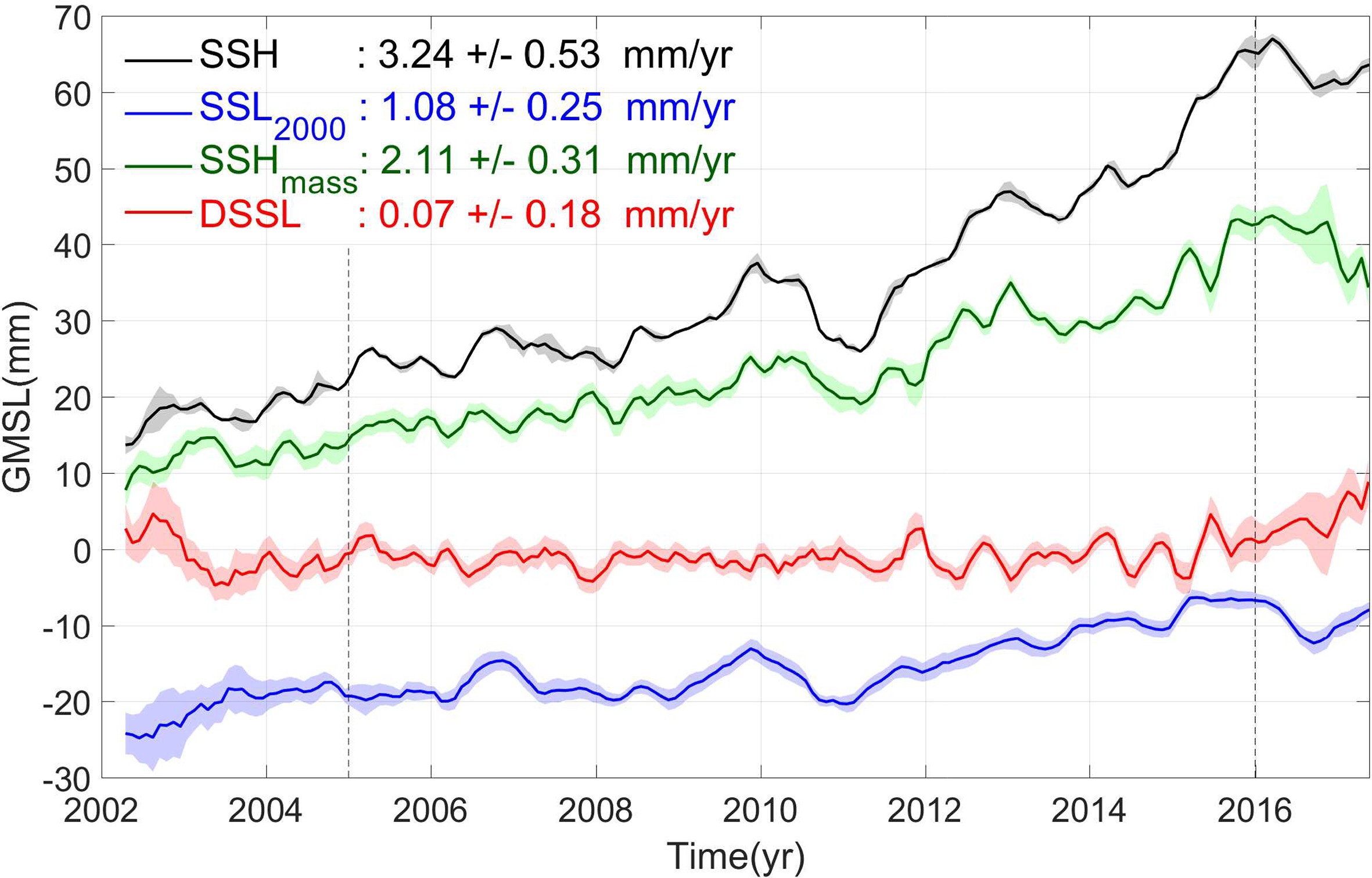Figure3. Time series of global mean sea level change including ${\rm{SSH}}$ (black line), ${\rm{SS}}{{\rm{L}}_{2000}}$ (blue line), ${\rm{SS}}{{\rm{H}}_{{\rm{mass}}}}$ (dark green line), and ${\rm{DSSL}}$ (red line). The solid lines represent the average of multiple datasets, and the corresponding shaded regions represent the standard deviation. The linear trend uncertainties (95% confidence interval) of each series from 2005 to 2015 are shown in the legend. We offset the time series for clarity.


Figure 4 depicts the spatial patterns of long-term trends in ${\rm{SSH}}$, ${\rm{SS}}{{\rm{L}}_{2000}}$, ${\rm{SS}}{{\rm{H}}_{{\rm{mass}}}}$, ${\rm{DSSL}}$, and OHC within the shallow (0–2000 m) and deep layers. The regional sea-level rate and its steric component show similar spatial patterns, such as the sea-saw mode in the Pacific (Royston et al., 2020) (Figs. 4a, b). In most oceans, the GRACE-based ocean mass increases slowly with a smaller magnitude of trend compared with altimetry and Argo (Fig. 4c). The regional DSSL change is not uniform and shows strong local patterns that can be 1–2 orders of magnitude larger than the global mean (Fig. 4d). The obvious positive trends are observed in the Middle East Indian Ocean (Region 1), the Tropical Northeast Pacific (Region 2), the subtropical Southwest and North Pacific (Region 3), the Kuroshio extension region, and the Northeast Atlantic (Region 5). The obvious negative trends appear in the Agulhas Basin, the Northwest Atlantic (Region 4), the South Atlantic, and the Southeast Pacific.
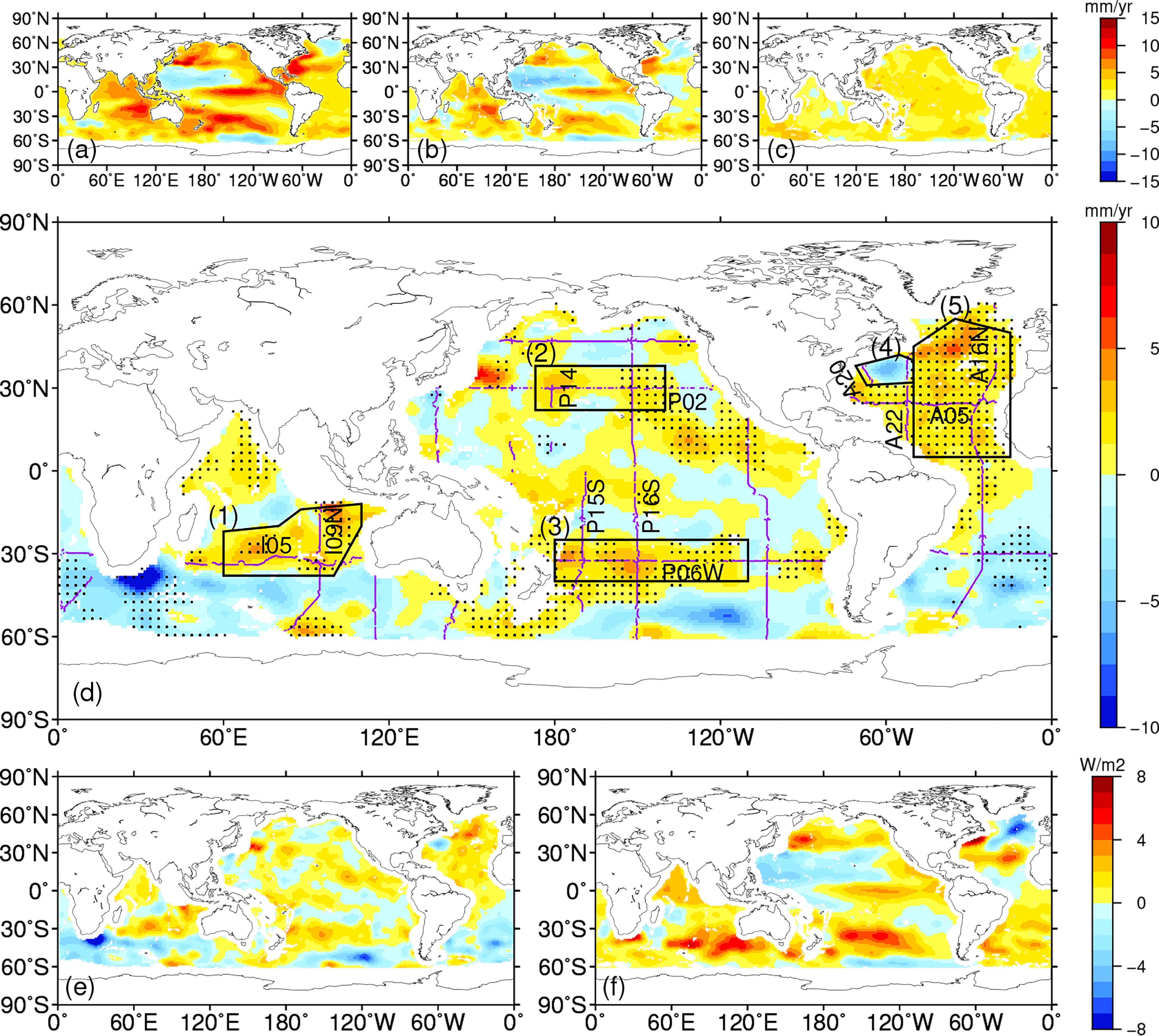Figure4. The estimated ensemble mean linear trend of (a) total sea-level change from altimetry, (b) steric sea-level change (0–2000 m) from Argo, (c) GRACE-based ocean mass change, (d) DSSL change from the residuals of “Alt.–Argo–GRACE” over the period 2005–15, deep OHC change (e) below 2000 m, and (f) above 2000 m. Note that (e) is derived from panel (d) under the ideal assumption that the DSSL change is entirely caused by the temperature change (more details in Section 2). The black boundaries in panel (d) outline the regions we selected for validation and the numbers in brackets represent the corresponding index of the regions. The purple points in panel (d) denote the repeated sections covering the GRACE era. The stipple dots in (d) denote the regions with significant trends (95% confidence interval). It should be noted that different color scales are used for panels (a–c) and panel (d).


Figure 4e shows the spatial pattern of OHC trends in the deep oceans from 2005 to 2015 (more details in Section 2), which is similar to that of DSSL changes in Fig. 4d since we assume that DSSL changes are attributed to temperature changes. Thus, a rising DSSL corresponds to a deep ocean warming and vice versa. By comparing this with the OHC trends in upper oceans (Fig. 4f), it is likely that the heat accumulated in the upper layers of the South Pacific, Indian Ocean, and the subtropical Atlantic Ocean has penetrated into the deep oceans during 2005–15 (Volkov et al., 2017). However, the opposite signs of OHC trends between the upper and deep layers appear in the sub-polar North Atlantic and South Atlantic, the Agulhas Basin, which may be related to the strong deep ocean circulations in these regions (Song and Colberg, 2011; Purkey and Johnson, 2013; Chen and Tung, 2018; Hu et al., 2020).
The contribution of the deep ocean to the global mean sea-level change is so small that most studies attribute the residual to observational errors. Even considering the basin scale, the SLB in most ocean basins can be closed within tolerance (Royston et al., 2020). Using a global average DSSL trend of 0.1 mm yr^?1 to close the regional SLB, Royston et al. (2020) found a SLB gap in the Indian-South Pacific region of up to 1.2 mm yr^?1, which exceeds the uncertainty caused by different data sets, processing, and corrections. Our study finds that this gap is due to significant deep warming from 2015 to 2016.
Although the selection of data products and post-processing strategies will inevitably affect the estimation of DSSL in most oceans, we still found some significant decadal regional DSSL changes highlighted in Fig. 4d. For example, the DSSL in subtropical Southwest Pacific increased at a rate of 1.80±0.77 mm yr^?1, which is consistent with the estimate of 2.40 ± 1.30 mm yr^?1 from Volkov et al. (2017). Our indirect rate is much closer to the estimation of repeated ship-based observation (Table 2), which is attributed to the adoption of multiple Argo datasets, as well as the updated GRACE RL06 and correction strategies.

Region index	Sections	time	Trends of GO-SHIP			Trends of Alt.-Argo-GRACE
			DSSL	DTSL	DHSL
1. Middle East Indian Ocean	I05	2002.4?2009.6	0.97	0.81	0.16	1.89 ± 0.67
	I09N	2007.3?2016.5	0.38	0.65	?0.26
2. subtropical North Pacific	P02	2004.7?2014.8	0.39	0.19	0.20	0.98 ± 0.74
	P14	2003.9?2015.9	0.82	0.18	0.65
	P16N	2006.3?2015.6	0.70	0.08	0.62
3. subtropical Southwest Pacific	P06W	2003.9?2010.3	0.21	0.03	0.18	1.80 ± 0.77
	P16S	2005.2?2015.7	0.98	0.64	0.34
	P15S	2009.3?2016.7	1.23	1.17	0.06
4. Northwest Atlantic	A20	2003.10?2012.6	?2.49	?2.91	0.42	?3.66 ± 1.98
	A22	2003.12?2013.4	?0.56	?1.10	0.54
5. Northeast Atlantic	A16N	2003.6?2013.12	0.84	0.56	0.28	2.01 ± 0.77
	A05	2010.1?2016.1	0.31	?0.21	0.52

Table2. Comparison of regional DSSL trend from direct and indirect methods in mm yr^-1.



2 -->

3.2. Impact of GRACE processing parameters on deep steric change

Previous studies highlighted the sensitivity that different post-processing strategies of GRACE have upon the spatial distribution of ocean mass change (Blazquez et al., 2018; Chen et al., 2018; Jeon et al., 2018; Mu et al., 2020; Royston et al., 2020). However, the uncertainties of the spatial pattern induced by different GRACE products and post-processing strategies are relatively uniform and smaller than the significant trend signals in DSSL (Fig. 5 and Table 3). Moreover, the STD of DSSL changes is mainly due to the discrepancies in Argo datasets, such as in the South Atlantic (Fig. 2), which indicates that the ensemble mean from multiple Argo datasets should be used as much as possible when using the indirect method to study DSSL.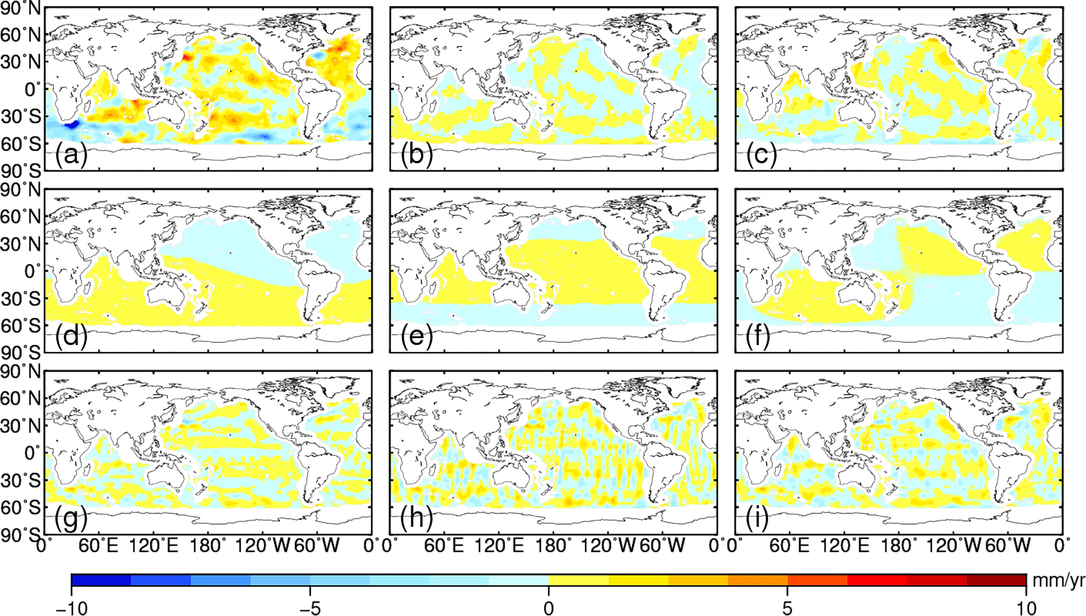
Figure5. Comparison of deep steric patterns with different GRACE processing strategies. (a) The ensemble mean of spherical harmonics and mascon solutions using the latest RL06 recommended processing strategy, which is used as the reference to be removed from the following panels (b–i). (b) Difference from (a) with only the ensemble means of spherical harmonic solutions from CSR, JPL, GFZ, and ITSG, (c) difference from (a) with only mascon solutions, (d) difference from (a) with another degree-1 correction (Swenson et al., 2008), (e) difference from (a) with another C20 correction (Cheng et al., 2013), (f) difference from (a) with another GIA model (A and Zhong, 2013), (g) difference from (a) with the Gaussian smoothing using a radius of 500 km, (h) difference from (a) with no destriping, (i) difference from (a) with another empirical destriping method (Swenson and Wahr, 2006).

Figure index	Region_index
	1: Middle East Indian Ocean	2: subtropical North Pacific	3: subtropical Southwest Pacific	4: Northwest Atlantic	5: Northeast Atlantic
5(a)	1.89 ± 0.67	0.98 ± 0.74	1.80 ± 0.77	?3.66 ± 1.98	2.01 ± 0.77
5(b)	2.10 ± 0.73	2.00 ± 1.43	2.50 ± 0.83	?3.96 ± 2.02	1.80 ± 0.85
5(c)	1.45 ± 0.59	1.41 ± 1.35	2.07 ± 0.65	?3.04 ± 1.95	2.41 ± 0.66
5(d)	2.77 ± 0.58	1.31 ± 1.39	3.03 ± 0.65	?4.60 ± 1.99	1.15 ± 0.71
5(e)	2.03 ± 0.67	1.90 ± 1.40	2.41 ± 0.74	?3.64 ± 1.98	2.11 ± 0.78
5(f)	2.28 ± 0.67	1.81 ± 1.39	2.30 ± 0.74	?3.39 ± 1.98	2.42 ± 0.77
5(g)	1.82 ± 0.67	1.73 ± 1.38	2.25 ± 0.74	?3.86 ± 2.00	1.95 ± 0.77
5(h)	1.56 ± 0.65	1.35 ± 1.39	2.14 ± 0.72	?3.44 ± 1.96	1.90 ± 0.77
5(i)	1.56 ± 0.67	172 ± 1.40	2.16 ± 0.73	?3.20 ± 2.00	1.89 ± 0.76

Table3. Comparison of regional deep steric trend (units: mm yr^?1) from different GRACE processing strategies described in Fig. 5.


We analyzed the effect of different GRACE solutions and post-processing strategies on the estimation of the deep steric change from 2005 to 2015. We used the GRACE post-processing parameter selection described in Section 2 as a reference or baseline scheme and analyzed the associated discrepancy on deep steric change estimation by replacing a specific parameter.
Figure 5 illustrates the sensitivity of deep steric change to the selection of GRACE processing parameters. There is no obvious difference in the pattern of deep steric change when we choose different types of GRACE products, i.e., spherical harmonic solutions or mascon solutions (Figs. 5b, c). The different correction of the first-order term and C20 will more or less enhance or weaken regional signals, but it will not change the spatial pattern of the obvious signal (Figs. 5d, e). Although the choice of the GIA model may affect the basin-scale SLB, it will not affect the spatial distribution of significant DSSL signals, such as North Atlantic (Fig. 5f). A larger filter radius will slightly weaken the signal, but it will not essentially change the pattern (Fig. 5g). The deep steric rate pattern will show obvious north-south stripes if a de-striping filter has not been applied to the GRACE data (Fig. 5h). The discrepancy of different GRACE empirical striping methods on the spatial distribution of deep steric is also negligible (Fig. 5i). Note that these processing methods may have a critical effect on some regions with plausible weak signals.
Table 3 lists the linear trends of regional deep steric change estimated by different GRACE solutions and post-processing strategies. As shown in Table 3, these subjective choices affect the indirectly estimated regional deep steric linear trends, which may exceed the order of 1 mm yr^?1. It is difficult to accurately estimate the regional deep steric change. Despite the potential spread caused by GRACE treatment, the deep steric change in these regions is significant at a 95% confidence interval. Note that these comparisons are intended to show the impact of potential GRACE treatment strategies, we recommend the latest GRACE processing strategies described in section 2.

2 -->

3.3. Validation of the deep ocean steric sea-level changes

To validate the regional DSSL changes, we selected five regions with significant signals (Fig. 4d) and compared the derived DSSL changes with GO-SHIP data. The criteria of the regional selection are: 1) there should be at least two repeated sections in the region to quantify the temporal change of the regional DSSL, and 2) the signal of cooling and warming in the selected areas are significant so the comparison is meaningful.
Figure 6a shows the spatial patterns of DSSL rates from the direct and indirect methods in the five selected regions. The DSSL changes along each track line are far from uniform, which is likely related to the rich eddies, tides, and waves (Volkov et al., 2017). Note that the color scales of the two methods are different, mainly associated with the smoothing effects of the indirect datasets (the typical spatial scale of the GRACE and Argo-based datasets are ~3 degrees but the direct measurements include variations from all scales). The differing smoothness of the two datasets challenges the strict comparison of the two methods, but we can still identify the consistency of the sign of the trends. As shown in Fig. 6b and Table 2, the meridional or zonal average trend along the track line reveals either a consistent increasing or decreasing trend. For example, the DSSL from the indirect method increased by a rate of 1.89±0.67 mm yr^?1, 0.98±0.74 mm yr^?1, 1.80±0.77 mm yr^?1 in the Middle East Indian Ocean, subtropical North Pacific, and subtropical Southwest Pacific, respectively, while the sections along these regions also captured coincident increasing rates ranging from 0.21 mm yr^?1 to 1.23 mm yr^?1. Most notable is the significant DSSL rise of 2.01±0.77 mm yr^?1 in Region 5 of the North Atlantic inferred from the indirect method, agreeing well with the track line A16N and the eastern part of A05 (Fig. 6a). The negative DSSL rate (–3.66±1.98 mm yr^?1) derived from “Alt.–Argo–GRACE” in the Northwest Atlantic, is also dramatically in line with the decreasing DSSL from the track line A20 and A22 (–2.49 mm yr^?1 and –0.56 mm yr^?1).
Figure6. Comparison between the direct and indirect DSSL trends for the (a) spatial pattern, (b) regional time series and trend lines from different methods and track lines, and (c) regional average trends over 2005–15. Note that different color bars are used for GO-SHIP and “Alt.–Argo–GRACE” in (a). In (b), the gray solid lines represent the average DSSL of multiple datasets from “Alt.–Argo–GRACE”, and the corresponding shaded area represents the standard deviation. The red lines show the trends from “Alt.–Argo–GRACE” fitted by the least-squares. Trend lines in other colors represent the corresponding estimates from track lines in the region. The error bars in (c) represent the uncertainty (95% confidence interval) of the least-squares fit for Alt.-Argo-GRACE and the spread around the ensemble mean from different sections for GO-SHIP.


The trend signs of DSSL changes obtained by these two independent methods are the same in the selected five regions (Fig. 6c), which demonstrates that the average result calculated based on the indirect method is reliable. The difference in magnitude between them may be due to the uncertainties in the GRACE and Argo data (Figs. 2 and 5), as well as the inherent observation errors associated with the gridded datasets. Moreover, the undersampling of GO-SHIP data in both the spatial and temporal domains, when compared to the indirect method, yields approximate cancellation between the positive and negative DSSL signals along the track lines, which may explain the smaller amplitude of DSSL trends from GO-SHIP CTD observations.
Furthermore, with the hydrographic temperature and salinity data, we can further test the impact of salinity change on the DSSL change and assess the potential to estimate deep ocean temperature changes. Figure 7 depicts the selected regional average trend of DSSL, the deep thermosteric sea-level (DTSL) caused by temperature variations, and the deep halosteric sea-level (DHSL) caused by salinity variations. In the Middle East Indian Ocean (Region 1), subtropical Southwest Pacific (Region 3), and Northwest Atlantic (Region 4), the temperature dominates the DSSL change; while the salinity contribution cannot be ignored in the subtropical North Pacific (Region 2), Northwest Atlantic (Region 4), and Northeast Atlantic (Region 5). In all these regions, the increased steric is consistent with an increase in temperature, and vice versa. The consistency of sign between DTSL and DSSL suggest that the DSSL rates from the indirect method can be used to infer the deep temperature changes and the warming or cooling in these regions.
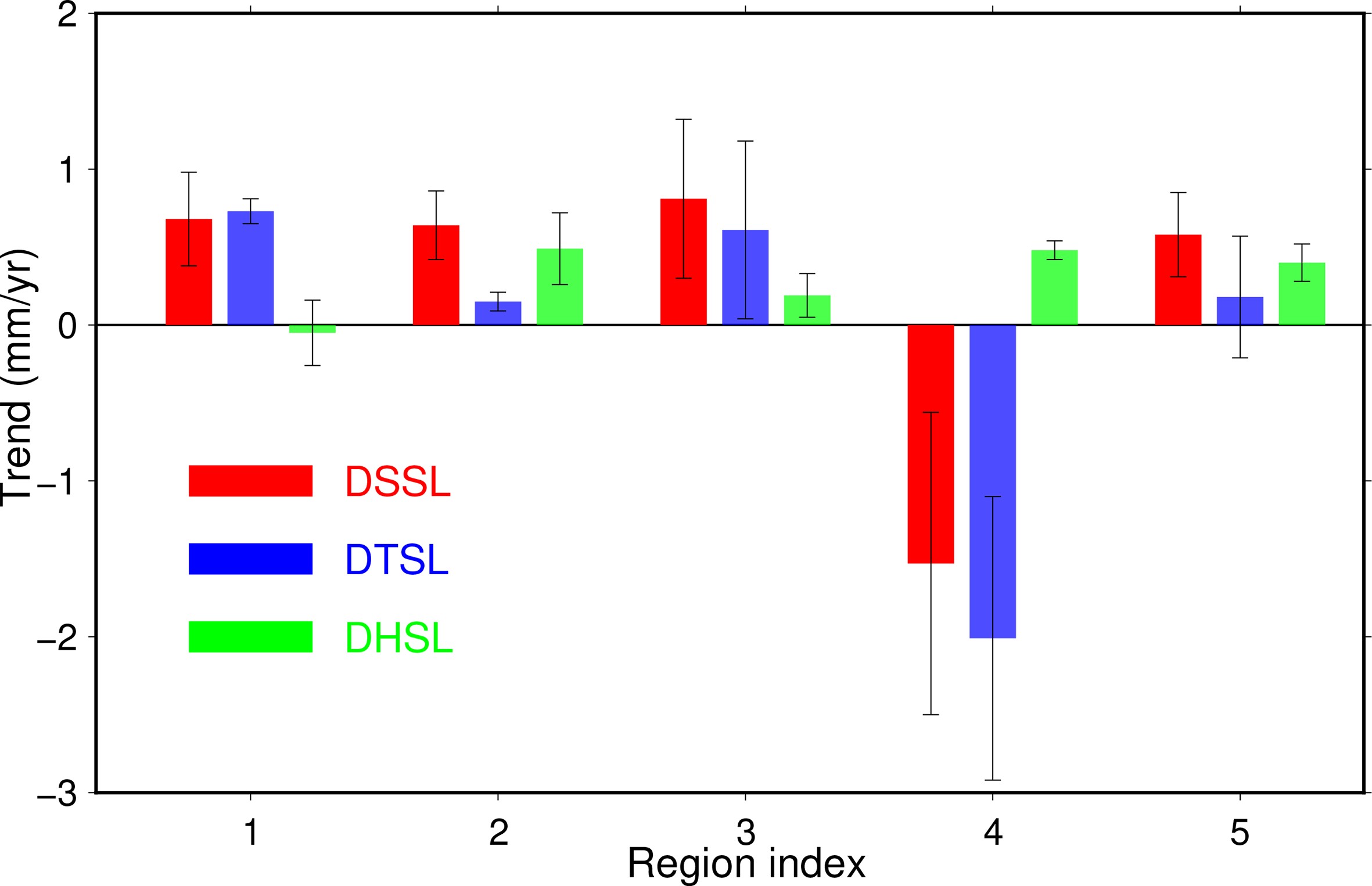Figure7. Comparison of trends in DSSL (red), DTSL (blue), and DHSL (green) in the five regions. Error bars represent the spread of the regionally averaged DSSL rate.


Although we provide a finer resolution estimate of the deep ocean temperature change pattern (Figs. 4 and 6), our finding corresponds well with many previous results, i.e., the evident deep ocean warming in the northeastern Atlantic Ocean during the period of 2002–10 using the data from six A25-Ovide cruises (Desbruyères et al., 2014). Warming signals in the abyssal southeastern Indian Ocean are captured by comparing repeated hydrographic sections between 1994–95 and 2007 (Johnson et al., 2008). In addition to the selected five regions, the indirect method also highlights the DSSL decrease i.e., ocean cooling in the Agulhas Basin, South Atlantic, and southeast Pacific (Fig. 4d). These changes are very similar to the SLB discrepancy pattern given by Royston et al. (2020), but they simply assume a global mean value of 0.1 mm yr^-1 for DSSL changes in all oceans. Using T waves generated by underwater earthquakes, a decadal warming trend was uncovered in the East Indian Ocean by Wu et al. (2020). The newly developed seismic ocean thermometry is expected to expand our ability to monitor ocean temperature changes. Moreover, the ongoing deployment of Deep Argo buoys may essentially solve this problem, which is also the focus of future research.
Climate warming has extended into most regions of the deep ocean, especially the Indian Ocean, the subtropical Southwest Pacific, and the northeast Atlantic from 2005 to 2015, while the deep ocean is cooling in Northwest Atlantic. However, due to the lack of in-situ measurements, significant steric changes in the Agulhas Basin, South Atlantic, and southeast Pacific from “Alt.–Argo–GRACE” cannot be validated independently.

In this study, regional DSSL changes were estimated from altimetry, GRACE, and Argo observations from 2005 to 2015. Different post-processing strategies of GRACE data will more or less enhance or weaken regional signals, but it will not change the spatial pattern of the obvious signal significantly. Significant deep ocean warming in the Middle East Indian Ocean, the subtropical North Pacific, the subtropical Southwest Pacific, and the Northwest Atlantic, and deep ocean cooling in the Northwest Atlantic are detected by “Alt.–Argo–GRACE”. The repeated hydrographic sections also confirmed these local significant DSSL changes. Our findings indicate that the indirect method can be used to detect potential local deep-warming or cooling. We also find that the sign of the thermosteric sea-level trend is consistent with that of the steric sea-level trend in these regions.
Although the indirect method has the potential to detect regional deep ocean warming, it is difficult to accurately estimate deep ocean warming or cooling quantitatively. On the one hand, the salinity effect in the deep ocean may enhance or weaken the DSSL signal obtained by the indirect method. We also find that the DHSL in some regions makes a comparable contribution to the DTSL, though is not enough to change the sign of the DSSL. On the other hand, the uncertainty of the ensemble is the variance between data products, which may not represent the true error. The datasets derived from in-situ observations have a certain level of uncertainty owing to instrumental biases and insufficient data coverage in some locations. These uncertainties are inherent, not independent, and hard to accurately quantify. Therefore, we recommend using independent methods and multiple data platforms to estimate and confirm deep ocean warming.
The results of the indirect method are highly dependent on the quality of the three data sources, which will be greatly improved in the foreseeable future. Deep Argo has demonstrated the near real-time and high-precision measurement capability, which can help us further validate the results of the indirect method. Seismic ocean thermometry provides clues to detect the potential deep ocean temperature changes with high temporal resolution (Wu et al., 2020). The significant signal regions detected by multi-source data can also be used as the basis for the Deep Argo deployment (Johnson et al., 2015). The acquisition of additional multi-source geodetic and oceanographic datasets with higher precision and spatiotemporal resolutions in the near future can further deepen our understanding of changes in ocean heat content and steric sea-level in deep oceans.
Acknowledgments. This work is supported by the National Natural Science Foundation of China (Grant No. 41904081). We thank the institutions (listed in Table 1) for sharing their data products used in this study. These data sets are available at the websites or references listed in Table 1. The authors declare no financial conflicts of interest. The authors comply with AGU's data policy. The data archiving is underway. The repository we plan to use is Global Change Research Data Publishing and Repository (GCdataPR, http://www.geodoi.ac.cn/WebEn/Default.aspx).