HTML
--> --> -->Although most of the models that participated in the last phase of CMIP (CMIP5) showed the ability to reproduce the general circulation of the global ocean and sea ice, some obvious biases still existed. The previous version of FGOALS-f3-L is FGOALS-s2, which also contributed to CMIP5. The sea surface temperature (SST) simulated by FGOALS-s2 in CMIP5 generally showed cold biases in the subtropics and warm biases along the western and eastern oceanic boundaries and Southern Ocean; the Pacific warm pool was weak and the cold tongue was excessive (Lin et al., 2013); the simulated sea surface salinity (SSS) showed freshwater biases in the middle latitudes and salty biases in the Southern Ocean (Lin et al., 2013); and the simulated transport of Atlantic meridional overturning circulation (AMOC) was unrealistic, which may contribute to the temperature and salinity biases (Lin et al., 2013). These model biases in FGOALS-s2 are also common in other CMIP5 models (Griffies et al., 2011; Danabasoglu et al., 2012; Taschetto et al., 2014; Wang et al., 2014). At high latitudes, the simulated sea ice in FGOALS-s2 also showed obvious biases. In the Arctic, the sea ice was underestimated due to strong vertical mixing and showed an intense seasonal cycle that was common in other CMIP5 models (Griffies et al., 2011; Jahn et al., 2012) but stronger in FGOALS-s2. In the Antarctic, the model underestimated sea ice throughout the year, which was also found in other CMIP5 models (Griffies et al., 2011).
There have been several generations of coupled climate models developed at the LASG/IAP, which have been widely used in many geoscience fields (Zhang et al., 1992; Yu et al., 2002, 2004; Bao et al., 2013). The Flexible Global Ocean–Atmosphere–Land System Model (FGOALS) refers to the recent generations of coupled models (Yu et al., 2004, 2011; Bao et al., 2013). FGOALS mainly consists of four components: an atmosphere model, a land model, an ocean model and a sea ice model, which can exchange surface fluxes via a coupler. FGOALS-s2 (Bao et al., 2013) is one of the previous generations of FGOALS models, the CMIP5 results of which were adopted in the Fifth Assessment Report of the Intergovernmental Panel on Climate Change (IPCC AR5) (Stocker et al., 2013) and the latest Special Report of Ocean and Cryosphere in Changing Climate (SROCC) for IPCC AR6 (
This paper mainly focuses on evaluating the climatology of oceanic circulation and sea ice simulated by the low-resolution coupled climate system model FGOALS-f3-L in the CMIP6 historical experiment. Thus, the FGOALS-f3-L and FGOALS-s2 simulations are compared with some of the latest observed data. The model biases and improvements of FGOALS-f3-L are highlighted, and the potential causes are briefly discussed.
The remainder of the paper is organized as follows: Section 2 provides an overview of the FGOALS-f3-L model and the experiments, as well as the observed data used in this study. The results of simulated oceanic circulation, biases and related surface fluxes in FGOALS-f3-L and FGAOLS-s2 are introduced in section 3. The simulated sea ice results are presented in section 4. Finally, a summary and discussion of this study are given in section 5.
2.1. Model
The coupled model of FGOALS-f3-L consists of four individual component models. The atmospheric component is FAMIL, which is the new generation of the AGCM developed at LASG/IAP for CMIP6 (He et al., 2019) and a successor to the atmospheric component in FGOALS-s2. An efficient finite volume dynamic core (FV3) was introduced into this model as well as several new parameterization schemes that have substantially improved the overall performances compared with the previous version (Li et al., 2019). The oceanic component is the LASG/IAP Climate System Ocean Model version 3.0 (LICOM3), the latest version of the OGCM developed at LASG/IAP for several generations (Zhang and Liang, 1989; Jin et al., 1999; Liu et al., 2004, 2012). Several improvements were introduced in LICOM3 compared with its previous version, LICOM2.0, adopted in FGOALS-s2, including a tripolar grid dynamic core (Yu et al., 2018), a preserved shape tracer advection scheme (Xiao, 2006), and several new parametrization schemes such as a buoyancy frequency (N2) related thickness diffusivity (Ferreira et al., 2004), a new vertical diffusivity (Canuto et al., 2001, 2002), and tidal mixing (St Laurent et al., 2002). Application of the tripolar grid solved the problems related to the longitude–latitude grid in the previous versions, e.g., the inability to simulate the North Pole and transpolar circulations (Li et al., 2017b). Hence, the capacity of the model to simulate high-latitude oceans was greatly improved (Li et al., 2017b). For the low-resolution sub-version used in FGOALS-f3-L, the horizontal resolution of LICOM3 is approximately 1° (360 × 218 grid points) with enhanced meridional resolution near the equator; the vertical resolution is 30 levels, which is 10 m per layer in the upper 150 m (Wu et al., 2005) and divided into uneven vertical layers below 150 m. The land component is the Community Land Model, version 4 (CLM4), (Lawrence et al., 2011) from the National Center for Atmospheric Research (NCAR). The sea ice component is the Community Ice Code, version 4 (CICE4) (Hunke and Lipscomb, 2010), which is an update of the Los Alamos Sea Ice Model. Some codes in CICE4 have been modified to adapt the tripolar grid of LICOM3 so that the horizontal grid of the sea ice model is consistent with the oceanic model. All the component models are coupled via Coupler 7 (Craig et al., 2012) from NCAR and the coupling frequency is 3 h for the oceanic model and 1 h for other component models. The main differences between FGOALS-f3-L and FGOALS-s2 are the atmospheric and oceanic models, which have been updated to the latest versions in FGOALS-f3-L for CMIP6 with remarkable changes in dynamic cores and physical schemes (He et al., 2019; Lin et al., 2020).2
2.2. Experiments and data
To generate proper initial fields for the historical experiments as well as test the stability of the model, the preindustrial experiment (piControl) was first conducted as required by CMIP6. The piControl experiment uses external forcing fixed at the level before industrialization (e.g., CO2 concentration is fixed at 284 ppm). In piControl, the oceanic model and sea ice model are initialized from a stable state obtained by an ocean–ice coupling experiment forced by atmospheric reanalysis data. Then, the coupled model is run for a relatively long period (in this study, the model was integrated for 1100 years) for piControl until the deep ocean approaches a stable state. Subsequently, the stability of the model was examined, showing that the model could reach stable oceanic and sea ice statuses after running for 500 years (not specifically discussed in this paper). Sequentially, using the stable fields generated by piControl as the initial fields (in this study, the results of piControl in the 600th, 650th and 700th year were used), three historical experiments are conducted under the historical forcing provided by CMIP6 (Matthes et al., 2017) that represent the realistic evolution of the external forcing (due to the CO2 concentration, land use, human activity, and so on) from 1850 to 2014. The output data of the historical experiments (Guo et al., 2020) have been submitted to CMIP6 and are now accessible to the public. In this paper, the results from only one historical experiment—the one started from the 600th year of piControl—are used to show the performance of the oceanic and sea ice models, thus avoiding the ensemble mean biases. The simulation of the historical experiment covers 165 years, but observed ocean and sea ice data are not widely available until the 1980s. Therefore, to compare the results with observations, the climatology of the simulated oceanic circulations and sea ice from 1980 to 2014 and the available observed climatology within this period are used in this study. In addition, the simulated climatology of FGOALS-s2 in CMIP5 historical experiments from 1980 to 2004 are also shown, to highlight the improvements of FGOALS-f3-L. The simulations of FGOALS-s2 were forced by the CMIP5 historical forcing data.Several of the latest observed ocean and sea ice datasets are used in this paper to evaluate the model simulations. For SST, the Extended Reconstructed SST dataset, version 4 (ERSST.v4) (Huang et al., 2015; Liu et al., 2015), is applied. For vertical ocean temperature and salinity, the World Ocean Atlas 2018 (WOA18) (Locarnini et al., 2019; Zweng et al., 2019) is used. For heat fluxes and water fluxes between the sea and air, the Objectively Analyzed Air–Sea Fluxes, version 3 (OAFLUX v3) (Yu et al., 2008) and the Global Precipitation Climatology Project version 2.3 (GPCP v2.3) (Adler et al., 2018) datasets are used. For wind stresses, the International Comprehensive Ocean–Atmosphere Data Set (ICOADS) (Freeman et al., 2017) is applied. The Rapid Climate Change Atlantic Meridional Overturning Circulation (RAPID-AMOC) dataset (Smeed et al., 2016) is used for AMOC, and the dataset from the World Ocean Circulation Experiment (WOCE) (Ganachaud and Wunsch, 2003) is used for meridional heat transport. Finally, the Bootstrap Sea Ice Concentrations from Nimbus-7 SMMR and DMSP SSM/I-SSMIS, Version 3 (SMMR/SSMI Bootstrap) (Comiso, 2017) are used to evaluate the sea ice simulations. All the observed data were interpolated onto the oceanic model grid of 360 × 218 and then compared with the model.
3.1. SST
Figure 1 shows the climatology of the simulated SST and its biases in FGOALS-f3-L (1980–2014) and FGOALS-s2 (1980–2004), as well as the observed SST. It is shown that the observed pattern of SST includes the western Pacific warm pool, cold tongue in the eastern equational Pacific and domains surrounded by the 0°C isotherm at high latitudes. Figure 1a shows that the FGOALS-f3-L simulation correctly captures the main observed global SST pattern, which implies that the simulated SST is reasonable on a global scale. Warm biases widely exist near western and eastern boundaries in FGOALS-s2 (Lin et al., 2013) as shown in Fig. 1b, which has been remarkably reduced in FGOALS-f3-L, showing significant improvements in simulated boundary SSTs. However, there were still some obvious biases in the simulated SSTs of FGOALS-f3-L. The global mean of simulated SST biases is ?0.41°C (maximum bias of 5.20°C, minimum of ?10.20°C), and the simulated root-mean-square error (RMSE) of SST is 1.31°C, which are both larger than in FGOALS-s2 (mean bias of ?0.04°C and RMSE of 0.90°C). In general, the simulated SST is slightly colder than observed. The strongest cold biases are mainly located over the mid- and high-latitude oceans in the Northern Hemisphere (NH), appearing in the northwestern Pacific, northwestern Atlantic, Labrador Sea, GIN (Greenland, Iceland and Norwegian) Sea and Barents Sea, which could be related to the overestimated sea ice that will be discussed in section 4. Some slightly cold biases appear at midlatitudes in all three oceanic basins in the Southern Hemisphere (SH). Cold biases at midlatitudes are also found in other CMIP5 models, which are usually associated with the disadvantage of simulating the extension of western boundary currents (Griffies et al., 2011; Bates et al., 2012). The western Pacific warm pool, the eastern equational Pacific and the western tropical Atlantic are also dominated by slight cold biases. The simulated Pacific warm pool is smaller and the cold tongue narrower and extended more to the west than in observations, which are common biases in many models (Taschetto et al., 2014). The largest warm biases are mainly located in the Antarctic Circumpolar Current (ACC) areas around Antarctica, and some slight warm biases appear in the eastern tropical Pacific surrounding the cold tongue and eastern boundary areas (e.g., western coasts of North America and Africa). Some narrow warm biases are also found in the western boundary coastal seas, such as the eastern coast of Japan, North America and South America.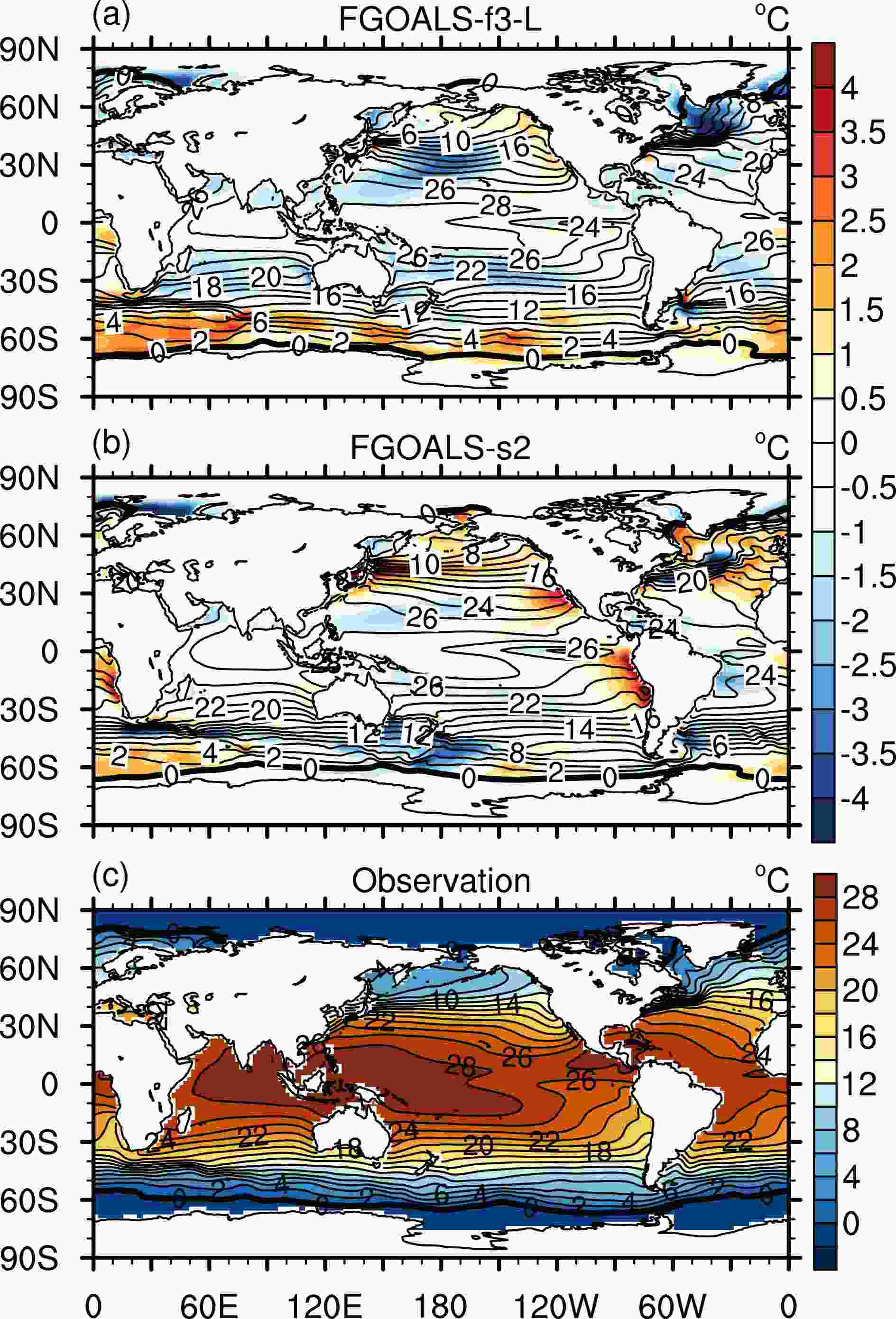 Figure1. Climatology of simulated SST (contours) and biases (shaded) in (a) FGOALS-f3-L (1980–2014) and (b) FGOALS-s2 (1980–2004), and (c) observed climatology of SST from ERSST.v4.
To reveal the origin and improvements in the simulated SST biases, the simulated biases of surface net heat flux, shortwave radiation and latent heat flux in FGOALS-f3-L (1980–2014) and FGOALS-s2 (1980–2004) are shown in Fig. 2. Overall, comparing the flux biases from these two models, FGOALS-f3-L and FGOALS-s2, it is apparent that the simulated biases in FGOALS-f3-L are generally smaller than those in FGOALS-s2, showing the progress of the new generation. In FGOALS-f3-L, in the midlatitude oceanic areas of both hemispheres (Northwest Pacific, Northwest Atlantic, and midlatitude oceans in the SH), which are dominated by cold SST biases, the simulated biases of net heat flux are positive, which means that the simulated ocean obtains more heat, and therefore the cold biases in these areas cannot be explained by local fluxes and should be related to the disadvantage of the model in simulating the location and intensity of western boundary currents due to the limited spatial resolution (Yu et al., 2012). The cold biases in the southern Labrador Sea might be related to the weak Gulf Stream, and the cold biases in the Northwest Pacific to the weak Kuroshio and its extension. However, the biases in the Kuroshio area near Japan are relatively small, which implies the simulated winter Asian monsoon is weaker than observed. The cold biases in the central midlatitude Pacific are strongly associated with the biases of mixed layer and wind stresses, which will be specifically discussed in section 3.3. However, the western Pacific warm pool and the western tropical Atlantic are dominated by negative biases of net heat flux, which would contribute to the slight cold SST biases there. In this case, the negative biases of net heat flux are mainly due to biases in latent heat flux. In the eastern boundary areas of the Pacific and Atlantic and the Southern Ocean, shortwave radiation is overestimated in FGOALS-f3-L, which might contribute to warm biases there, but the overestimation has been remarkably reduced from a maximum over 75 W m?2 to one that is under 50 W m?2 compared with FGOALS-s2, which shows the improvements of the physics such as the convection, cloud and boundary layer in the atmospheric model (He et al., 2019). The shortwave radiation of the Labrador Sea, GIN Sea and Barents Sea is underestimated in FGOALS-f3-L, which might also contribute to cold biases and be related to the overestimated sea ice there. Nevertheless, in a coupled model within complex interactions, the fundamental reasons behind SST biases still need to be further explored based on the circulations and detailed physical processes with further numerical experiments.
 Figure2. Simulated biases of surface net heat flux (positive downward) in (a) FGOALS-f3-L (1980–2014) and (b) FGOALS-s2 (1980–2004); the simulated biases of shortwave radiation at the sea surface (positive downward) in (c) FGOALS-f3-L and (d) FGOALS-s2; and the simulated biases of latent heat flux (positive downward) in (e) FGOALS-f3-L and (f) FGOALS-s2. The contours show the areas where biases are more than 25 W m?2. The observed net heat flux, shortwave radiation and latent heat flux are from OAFLUX v3 (1983–2009).
2
3.2. SSS
Figure 3 shows the climatology of the simulated SSS and its biases in FGOALS-f3-L (1980–2014) and FGOALS-s2 (1980–2004), as well as the observed SSS from WOA18 (1985–2017). It can be seen that the observed pattern of SSS mainly includes the high SSS in the subtropical oceans due to high evaporation and low SSS in the intertropical convergence zone due to abundant precipitation. Figure 3a shows that FGOALS-f3-L can reproduce the observed global SSS pattern, as the simulated maximal SSS values are located in the subtropical Atlantic, similar to observed. Compared with the biases of FGOALS-s2 shown in Fig. 3b, FGOALS-f3-L shows improvements at the eastern oceanic boundaries and in the subtropical northern Atlantic where the overestimation in FGOALS-s2 has been much reduced. The freshwater biases in the Barents Sea have also reduced remarkably, but the simulated SSS shows new freshwater biases in the Southern Ocean and the global mean bias is larger in FGOALS-f3-L. Besides, there are still some obvious biases in the FGOALS-f3-L simulation. Globally, the simulation underestimates the SSS in most areas except in the Arctic. Salty biases in the Arctic are common in CMIP5 models (Johns et al., 2006; Griffies et al., 2011), but the biases in FGOALS-f3-L are relatively larger. The global mean of the simulated SSS biases is ?0.71 psu, and the simulated RMSE of SSS is 1.62 psu. The freshwater biases are mainly located in the western Pacific, northwestern Atlantic, GIN Sea and Barents Sea, and most of the subtropical oceans in the SH including the western coast of Australia and southern Atlantic. Several small areas of salty biases also exist in the Bay of Bengal, western Pacific and western Atlantic.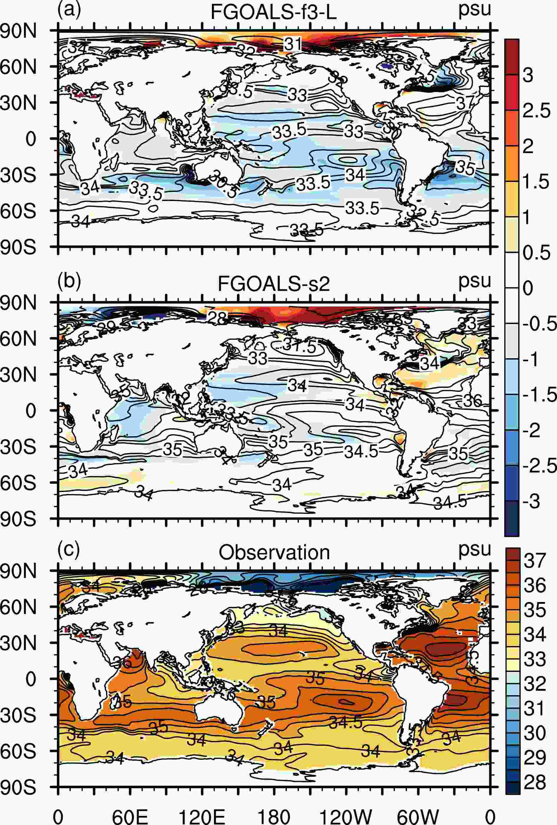 Figure3. Climatology of simulated SSS (contours) and biases (shaded) in (a) FGOALS-f3-L (1980–2014) and (b) FGOALS-s2 (1980–2004), and (c) observed climatology of SSS from WOA18 (1985–2017).
The simulated biases of evaporation minus precipitation (E-P), evaporation and precipitation in FGOALS-f3-L (1980–2014) and FGOALS-s2 (1980–2004) are shown in Fig. 4 to aid in understanding the origin of the simulated biases of SSS. Comparing the FGOALS-f3-L and FGOALS-s2 simulations, the E-P bias patterns are similar, but the former are lower, which demonstrates the improvements of the new version. Besides, although the SSS of the Southern Ocean in FGOALS-s2 seems to be more reasonable, it may only be a result of the overestimated E-P there; but in FGOALS-f3-L, the E-P biases of the Southern Ocean are lowered, which may cause the SSS biases in FGOALS-f3-L to become larger. Most of the negative SSS biases in the tropical and subtropical oceans in FGOALS-f3-L can be explained by the local negative E-P biases, except along the western coast of Australia and in the southern Atlantic. As the simulated evaporation is generally overestimated in the tropical and subtropical oceans in FGOALS-f3-L, the negative biases of simulated E-P are mainly due to the overestimated precipitation in these areas. The negative SSS biases along the western coast of Australia and in the southern Atlantic cannot be explained directly by the E-P biases. The dominant factor of these biases might be the oceanic dynamics, such as biases in meridional water transport near the ACC, but this remains to be further explored in the future. The negative SSS biases in the northwestern Atlantic are mainly due to negative E-P biases caused by low evaporation that could be related to the overestimated sea ice there. Besides, the salty boundary SSS biases could also be explained by the positive E-P biases there.
 Figure4. Simulated biases of E-P (evaporation minus precipitation, positive upward) in (a) FGOALS-f3-L (1980–2014) and (b) FGOALS-s2 (1980–2004); the simulated biases of evaporation (positive upward) in (c) FGOALS-f3-L and (d) FGOALS-s2; and the simulated biases of precipitation (positive downward) in (e) FGOALS-f3-L and (f) FGOALS-s2. The contours show the areas where biases are more than 40 cm yr?1. The observed evaporation is from OAFLUX v3, and the observed precipitation is from GPCP v2.3.
2
3.3. Mixed layer depth
The sea surface and oceanic deep layers are mainly connected by the upper boundary layer or mixed layer. Therefore, the mixed layer plays an important role in oceanic dynamics and air–sea interactions. The mixed layer depth (MLD) is an effective measure of mixing strength, which is impacted by wind stresses, heat and freshwater fluxes. The MLD shows significant seasonal changes, so the annual mean MLD is not a good way to indicate its features. Instead, in this study, the annual maximal MLD was calculated to show the features of the MLD.Figure 5 shows the climatology of the simulated maximal MLD in FGOALS-f3-L (1980–2014) and FGOALS-s2 (1980–2004), the observed maximal MLD derived from WOA18 (1985–2017), and the simulated biases. The MLD was defined as the depth where the potential density change exceeds 0.03 kg m?3, compared to the reference layer at 10 m. The simulated climatology of wind stress and its curl in FGOALS-f3-L are also shown in Fig. 6, along with the observations from ICOADS (1980–2014). In the tropics, the observed MLDs are shallow in the Pacific, Indian and Atlantic oceans due to weak stirring caused by weak wind stresses and strong solar radiation. At mid and high latitudes, due to strong wind stirring and less solar radiation, the observed MLDs are relatively deep in the northwestern and southeastern Pacific, northern Atlantic and Southern oceans.
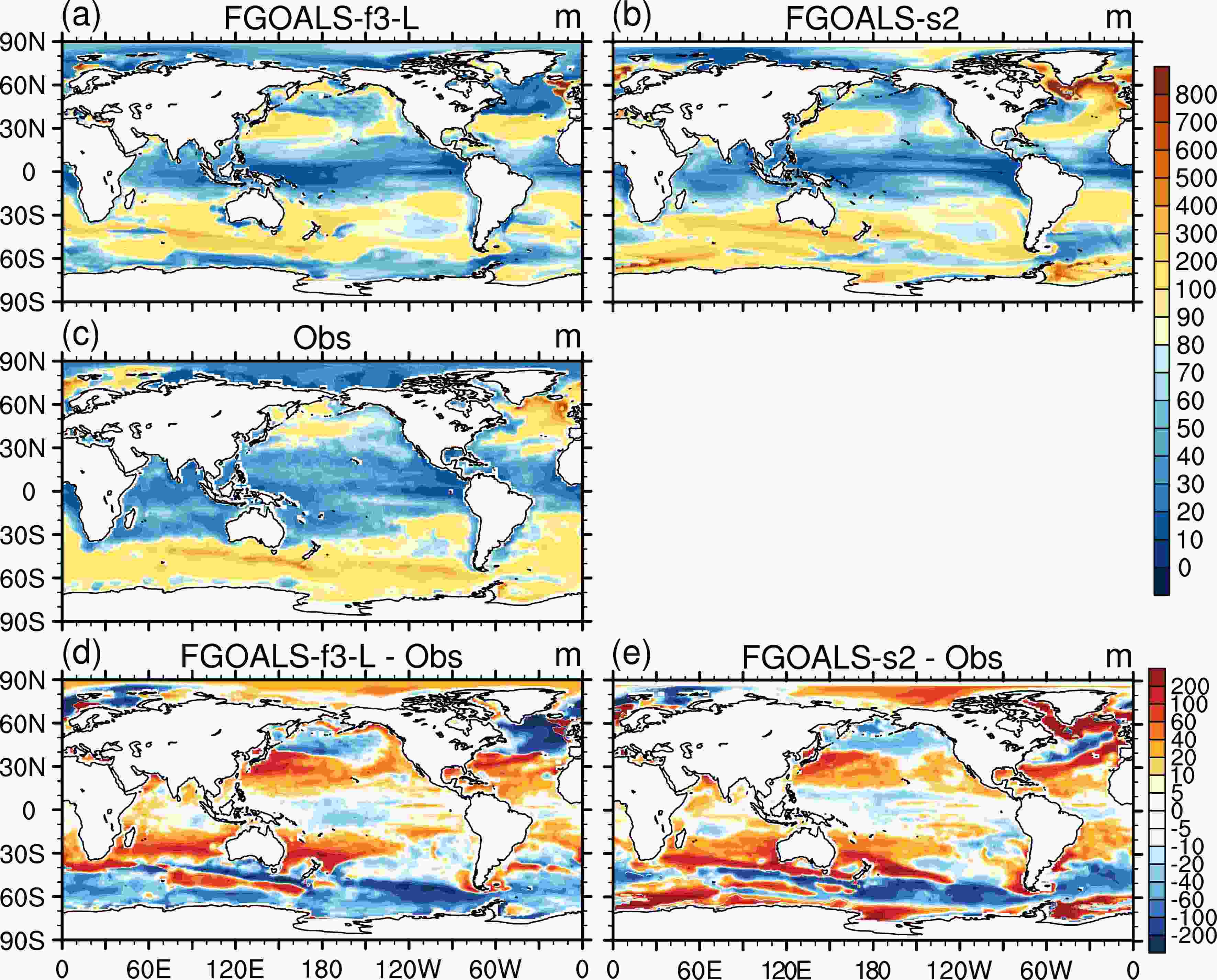 Figure5. Climatology of simulated maximal MLD in (a) FGOALS-f3-L (1980–2014) and (b) FGOALS-s2 (1980–2004); (c) the observed maximal MLD derived from WOA18 (1985–2017); and the simulated biases of maximal MLD in (d) FGOALS-f3-L and (e) FGOALS-s2. MLD is defined as the depth where the potential density change exceeds 0.03 kg m?3 compared to the reference layer at 10 m.
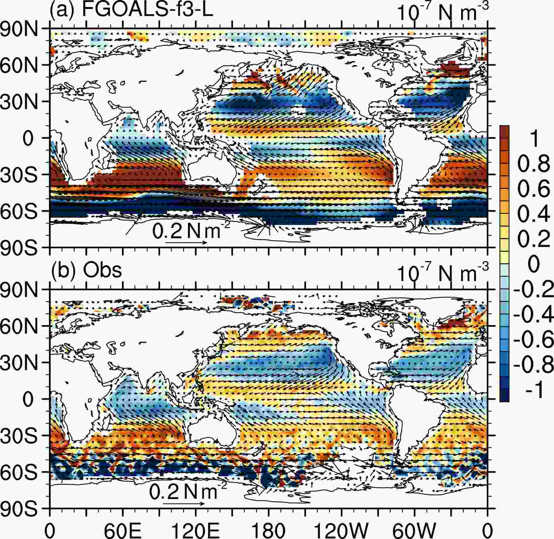 Figure6. Climatology of (a) simulated wind stress (vectors, N m?2) and its curl (shaded, 10?7 N m?3) in FGOALS-f3-L (1980–2014) and the (b) observed wind stress (vectors, N m?2) and its curl (shaded, 10?7 N m?3) from ICOADS (1980–2014).
Compared with the simulation of FGOALS-s2, the simulated MLDs in FGOALS-f3-L show a similar pattern, and the most obvious differences are mainly located at high latitudes. In the Southern Ocean near the Antarctic and northern Atlantic, the simulated MLDs in FGOALS-f3-L mainly show shallow biases, while the MLDs in FGOALS-s2 show deep biases. These differences are mainly due to the adjustments in convection mixing schemes in FGOALS-f3-L aimed at reducing the overestimated mixing processes at high latitudes in FGOALS-s2. The adjustments work well and successfully reduce the mixing strength, making the pattern of MLD more realistic at high latitudes, especially in the ocean near Antarctica, as well as reducing the biases in salinity and temperature in the deep ocean (see section 3.4). However, the adjustments also make the simulated mixing processes in FGOALS-f3-L weak and lead to shallow MLD biases at high latitudes, which need to be improved in future versions.
The simulated distribution of MLDs in FGOALS-f3-L agrees with the observation, albeit with the existence of some significant biases. In the tropics, MLDs are overestimated in the western Indian, tropical eastern Pacific and western Atlantic oceans, which could be related to the simulated strong wind stresses in FGOALS-f3-L. At mid and high latitudes, FGOALS-f3-L overestimates the MLDs in most subtropical oceans and underestimates them in the subpolar oceans, such as the northern Pacific, northern Atlantic and Southern oceans. A possible explanation for the overestimation in the subtropics is the simulated strong wind stresses; plus, the simulated cold SST biases there would also increase the potential density of the reference layer and contribute to the biases. Besides, the anomalous Ekman downwelling caused by the anomalous curl of anticyclonic wind stresses in the subtropics, which is indicated by the simulated stronger tropical easterlies and midlatitude westerlies, can also contribute to the deep MLD biases there. Additionally, the cold SST biases in the central midlatitude Pacific mentioned in section 3.1 are also related to the deeper mixed layer and the stronger anticyclonic wind stress curl that potentially cause excess meridional cold advection by Sverdrup transport. The subpolar shallow MLD biases are mainly related to the weak mixing as mentioned above, but it is notable that in the ocean from the northern Atlantic to the Barents Sea, the simulated MLDs mainly show strong, shallow biases, except for a small area in the eastern Atlantic at approximately 60°N where strongly deep biases exist. This abnormal distribution of MLD biases might be related to the overestimated sea ice located there (see section 4.1), which could influence the formation of deep water.
2
3.4. Vertical structures of temperature and salinity
The vertical structures of temperature and salinity are important metrics of a model’s performance for reproducing oceanic circulation in deep layers. Figure 7 shows the simulated global zonal mean temperature, salinity and simulated biases in FGOALS-f3-L (1980–2014) and FGOALS-s2 (1980–2004).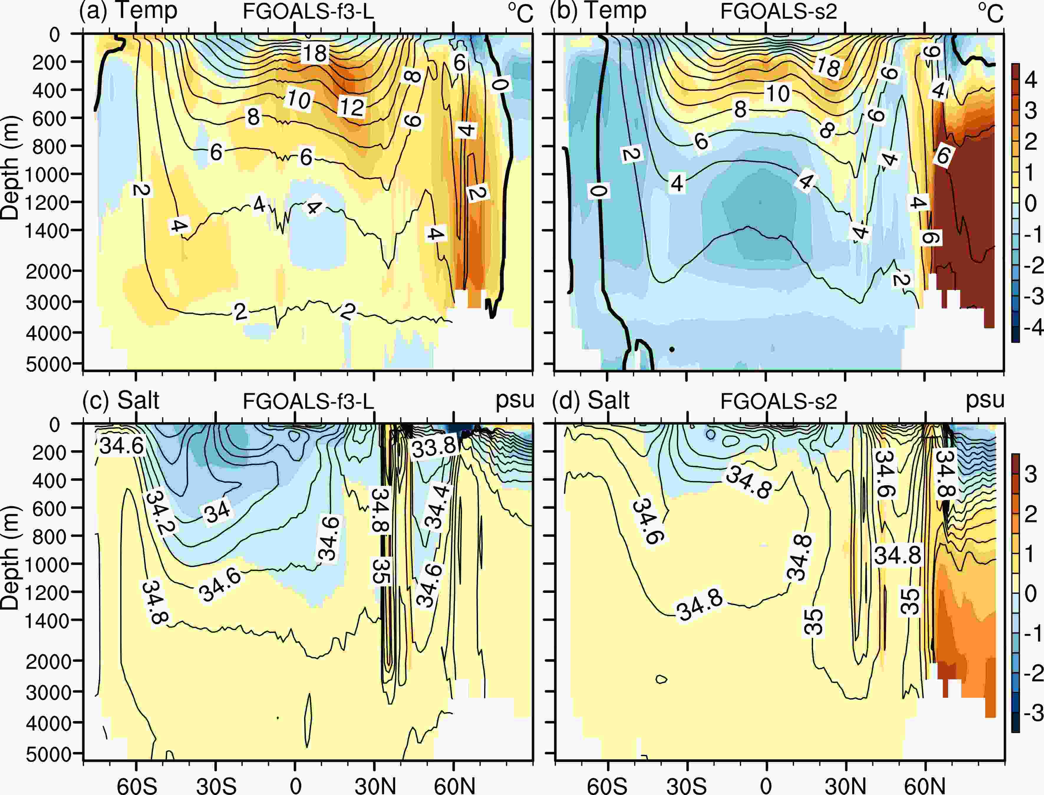 Figure7. Simulated global zonal mean temperature (contours) and biases (shaded) in (a) FGOALS-f3-L (1980–2014) and (c) FGOALS-s2 (1980–2004), in which the thick line represents 0°C; and the simulated global zonal mean salinity (contours) and biases (shaded) in (b) FGOALS-f3-L and (d) FGOALS-s2. The observed climatology is from WOA18 (1985–2017).
The simulated vertical temperature structure of FGOALS-f3-L, shown by the contours in Fig. 7a, is generally consistent with observations, e.g., the uplifted isotherms in the tropics, the concave isotherms in the subtropics, and the vertically well-mixed temperature and salinity at high latitudes. The biases of the simulated vertical temperature depend on the depth. At the surface, cold biases dominate most latitudes except in the Southern Ocean and the ocean from 0° to 10°S. At mid and low latitudes from 100 m to 600 m, where the tropical thermocline is located, warm biases dominate from 20°S to 30°N and can extend to 1000 m at 30°N, while cold biases connected to the surface exist from 20°S to 30°S above 400 m. These warm (cold) biases could be related to the deep (shallow) MLD biases there. In the deep layers under 600 m, slight warm biases dominate most of the ocean except at 10°N around 1400 m. There are obvious vertical temperature biases at high latitudes, including deep warm biases at 60°N under 300 m, deep cold biases north of 70°N from the surface to 1000 m, and deep cold biases south of 60°S from 200 m to 1200 m. The deep biases at high latitudes in the NH are also the most obvious biases in the simulation. Comparing the model biases from FGOALS-f3-L with those from FGOALS-s2, they are similar in the upper layers at mid and low latitudes, and their differences are mainly located in deep layers and at high latitudes. In FGOALS-s2, the biases in deep layers are strong, including cold biases south of 60°N and warm biases north of 60°N, which are caused by the strong mixing that brings more cold water to deep layers and influences the water exchange between the Atlantic and Arctic oceans. Given the weakened mixing in FGOALS-f3-L, the deep, strong, cold biases in FGOALS-s2 have been fixed and turned into slight warm biases, which demonstrates significant improvements in simulating the deep temperature. Meanwhile, the warm biases north of 60°N remain, which shows the model’s difficulty in simulating the water exchange between the Atlantic and Arctic oceans—an aspect that needs to be improved in future versions.
The structure of vertical salinity reflects the status of the water masses. As shown in Fig. 7b, the simulated zonal mean salinity in FGOALS-f3-L captures the main observed structure, including the low salinity from the surface to 2000 m south of 60°N that extends southward under 2000 m, which shows the North Atlantic Deep Water (NADW); the low salinity from the surface to 1400 m north of 60°S that extends northward, which shows the Antarctic Intermediate Water (AAIW); and the low salinity from the surface to the sea bed south of 60°S, which shows the Antarctic Bottom Water (AABW). Compared with the FGOALS-s2 simulation, the salinity structure in deep layers, including the southward extension of NADW and the appearance of AABW, is better captured in FGOALS-f3-L. The simulated biases of vertical salinity are also dependent on depth. Between 60°S and 30°N, the salinity shows freshwater biases above 1000 m, which could be related to heavy rain and weak mixing, and salty biases under 1000 m. At 60°S and 40°N, there are salty biases from the surface to the bottom. To the south of 60°N, freshwater biases exist from the surface to 1200 m, while salty biases exist under 1200 m, which could also be related to weak mixing in the model. At 60°N, strong freshwater biases exist in the surface layers above 200 m, which could be related to the overestimated sea ice extent, while salty biases exist under 200 m. North of 60°N, the upper layer shows freshwater biases and the deep layers under 500 m show salty biases. Comparing the simulated biases in FGOALS-f3-L and FGOALS-s2, the main differences are at high latitudes in the NH. As the mixing weakened in FGOALS-f3-L, the deep, salty biases in FGOALS-s2 south of 60°N, where the deep water forms, turns into slight freshwater biases, and the salty biases in the deep layers north of 60°N are remarkably reduced in FGOALS-f3-L, showing improvements in simulating deep salinity.
2
3.5. Meridional overturning circulations and meridional heat transports
The meridional overturning circulations (MOCs) and related meridional heat transports (MHTs) play important roles in the global energy balance. Figure 8 shows the simulated global meridional overturning circulation (GMOC), AMOC, and the simulated and observed AMOC at 26.5°N in FGOALS-f3-L (1980–2014) and FGOALS-s2 (1980–2004). FGOALS-f3-L captures the structures of GMOC and AMOC well, as observed (Lumpkin and Speer, 2007) or simulated in other CMIP5 models (Griffies et al., 2011; Danabasoglu et al., 2012; Cheng et al., 2013). The simulated main structure of MOCs include the tropical–subtropical cells in the upper 500 m, the Deacon cell and subpolar cell from the surface to 3500 m, the AABW below 2000 m in GMOC, and the NADW in GMOC and AMOC. As shown in Fig. 8e, the simulated AMOC at 26.5°N in FGOALS-f3-L has a similar vertical structure to the observation, which shows northward transport in the upper ocean and southward transport in the lower ocean. The simulated values of upper and lower transports are larger, and the depth of maximal transports is higher than observed, which are common biases in other CMIP5 models (Griffies et al., 2011). The observed AMOC northward transport at 26.5°N reaches a maximum of 16.7 Sv at approximately 1000 m, while the simulated northward transport reaches a maximum of 19.6 Sv at approximately 700 m. The observed southward transport reaches a maximum of 1.0 Sv at 5000 m, while the simulated southward transport reaches a maximum of 7.4 Sv at approximately 4000 m. Comparing the simulations of FGOALS-f3-L and FGOALS-s2, the structures of MOCs are similar, and the main differences are in the strength of transports. The northward transports of GMOC and AMOC in FGOALS-f3-L are intensified, while the southward transports of GMOC are weakened, and the depth of maximal northward transports is higher, which shows the influence of the weakened mixing in FGOALS-f3-L. Figure8. Simulated (a, b) GMOC and (c, d) AMOC in (a, c) FGOALS-f3-L (1980–2014) and (b, d) FGOALS-s2 (interval: 4 Sv), and the simulated (red curves) and observed (black curves) AMOC at 26.5°N in (e) FGOALS-f3-L and (f) FGOALS-s2. The observation is RAPID-AMOC (2004–2014).
The meridional circulations can transport warm water from low latitudes to high latitudes on the surface and cold water from high latitudes to low latitudes in the deep ocean, resulting in poleward heat transport in the ocean, which helps to maintain Earth’s meridional heat balance. Figure 9 shows the simulated MHTs in FGOALS-f3-L (1980–2014) for the global, Atlantic, and Indo-Pacific oceans. The observed estimates and errors (Ganachaud and Wunsch, 2003) are shown using black crosses and lines. Globally, heat is mainly transported from the equator to the poles, except for the cross-equatorial transport in the Atlantic, and the heat transport in the NH is stronger than that in the SH. The maximal global MHT is located south of 20°N with a value of 1.8 PW, which is close to the estimates from WOCE at 22°N. At 45°N, where observations are available, the simulated MHT is larger, whereas in the SH the simulated MHT is smaller than the observed locations at 20°S and 30°S. In the Atlantic, heat is mainly transported northward to north of 35°S. North of 20°S, the simulated MHT in FGOALS-f3-L is underestimated, while south of 20°S the simulated MHT is slightly overestimated. The underestimation of Atlantic MHT could be related to the underestimation of AMOC mass transport (Fig. 8e), as the warm biases in the upper Southern Ocean would strengthen the Atlantic MHT, which is a common problem in CMIP5 models (Griffies et al., 2011). The underestimation is also apparent in the recent OMIP (Ocean Model Intercomparison Project) experiments in CMIP6 and might be attributable to the coarse horizontal resolution (Chassignet et al., 2020), indicating this is a common obstacle within oceanic models. In the Indo-Pacific Ocean, the simulated northward MHT in the NH is overestimated, and the southward MHT in the SH is underestimated at the observed locations. No obvious difference exists between the FGOALS-f3-L and FGOALS-s2 simulations, so the simulated MHTs in FGOALS-s2 are not shown here.
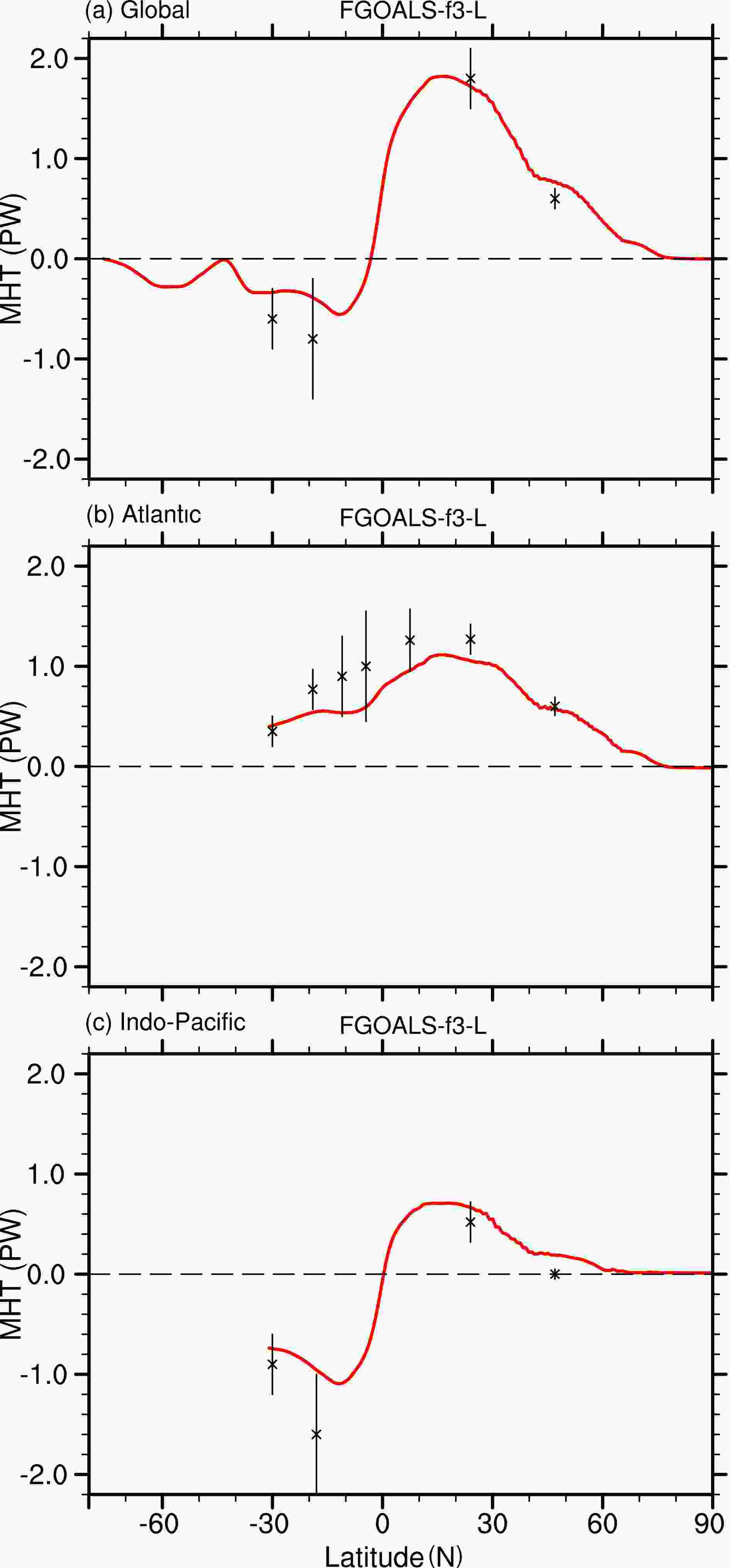 Figure9. Simulated (a) global, (b) Atlantic and (c) Indo-Pacific meridional heat transports (1 PW = 1015 W, positive northward) in FGOALS-f3-L (red curves, 1980–2014). Black crosses and lines are observed estimates and errors from WOCE.
4.1. Arctic
Sea ice is a critical factor in the high-latitude climate due to its effects on the exchange of sea–air fluxes and albedo on the surface. The capacity of simulating sea ice can greatly influence the performance of a coupled climate model at high latitudes. Figure 10 shows the climatology of the simulated and observed Arctic sea ice concentration (SIC) of FGOALS-f3-L (1980–2014) and FGOALS-s2 (1980–2004) in winter (February) and summer (September), as well as the simulated and observed seasonal cycle of sea ice extent.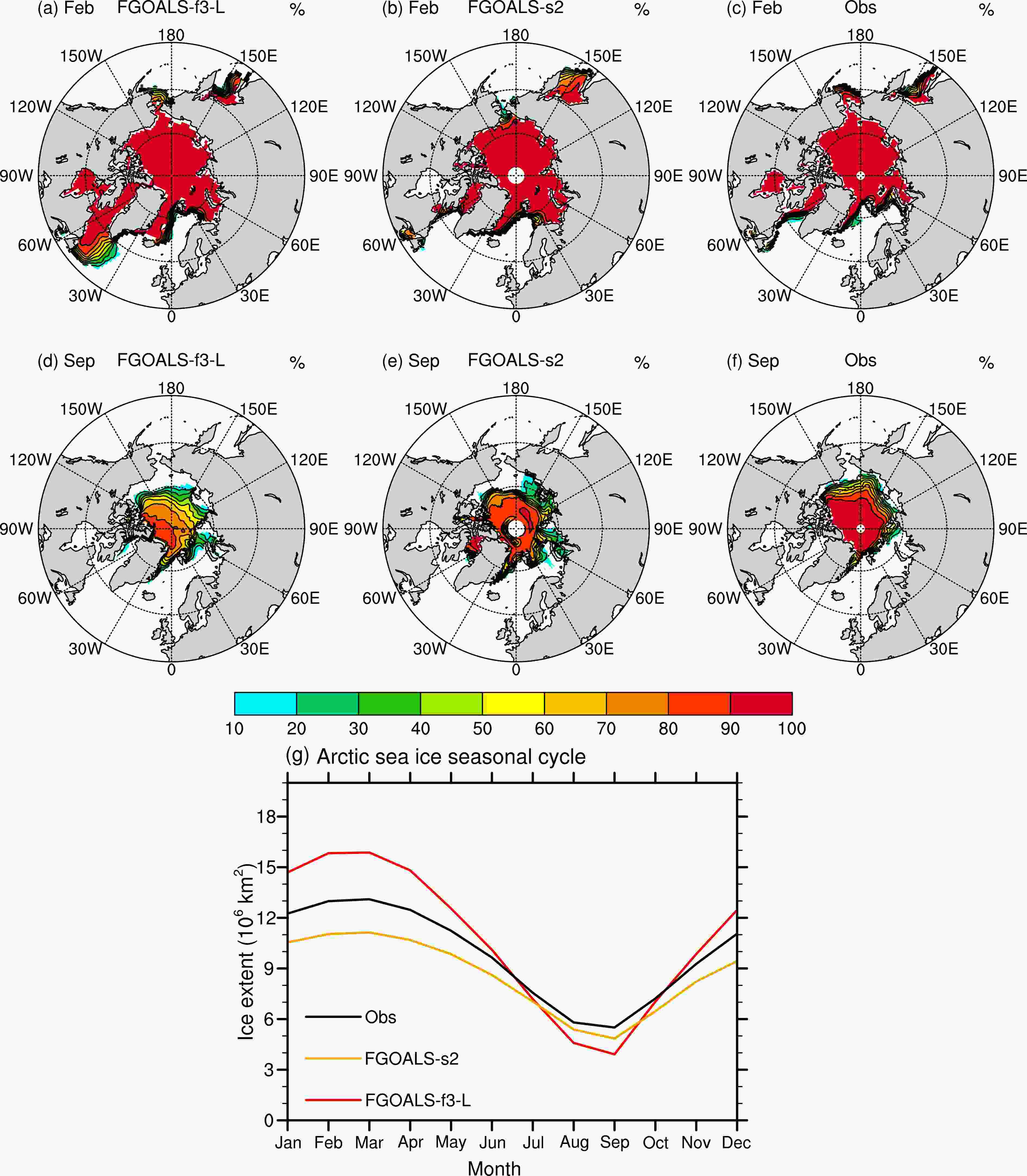 Figure10. Simulated sea ice concentrations (%) of (a, d) FGOALS-f3-L (1980–2014), (b, e) FGOALS-s2 (1980–2004) and (c, f) observations for the Arctic in (a–c) February and (d–f) September; and (g) the simulated seasonal cycle of sea ice extent (106 km2) in FGOALS-f3-L and FGOALS-s2, as well as the observation, for the Arctic. The observed sea ice concentration is from SMMR/SSMI Bootstrap; the sea ice extent is defined as the accumulated area where the sea ice concentration exceeds 15%.
As shown in Figs. 10a and d, FGOALS-f3-L can reproduce the general spatial distribution of sea ice in winter or summer, including the high SIC and large area in winter and low SIC and small area in summer. However, the simulated Arctic sea ice in FGOALS-f3-L still shows significant biases. The most obvious biases are located in the Labrador Sea, GIN Sea and Barents Sea, where the simulated winter sea ice shows a remarkably larger area than observed (Fig. 10a). Despite the overestimation of winter sea ice, which is a common bias in some CMIP5 models (Griffies et al., 2011; Jahn et al., 2012), the biases in FGOALS-f3-L are notably larger than those in other models, especially in the Labrador Sea. These significant overestimated biases are located exactly at the same locations where the aforementioned significant cold SST biases and freshwater SSS biases appear, which suggests a close relationship between the ice biases and SST or SSS biases. In addition, the overestimated sea ice could be related to the weakened vertical mixing and formation of deep water in FGOALS-f3-L at these locations, since weak mixing is an obvious source of coldness in the coupled model and thus might be related to the biases of temperature, salinity and MLDs. The spatial pattern of simulated sea ice in summer (Fig. 10d) is more realistic than in winter but, compared with observations, the simulated SIC is significantly lower, especially in the central area of sea ice, where the observed SIC exceeds 90% but the simulated SIC even reaches less than 80%. Additionally, the significant overestimation of sea ice extent in winter and the weak underestimation in summer are also found in the seasonal cycle of Arctic sea ice extent (Fig. 10g), showing an intensified seasonal cycle simulated by FGOALS-f3-L.
In contrast to the FGOALS-s2 simulations, FGOALS-f3-L can simulate the sea ice at the North Pole, due to the employment of a tripolar grid. However, the overestimation of winter sea ice in the Labrador Sea by FGOALS-f3-L is a new bias that was present in FGOALS-s2. In summer, the underestimation of SIC in the central Arctic in FGOALS-f3-L is generally stronger than that in FGOALS-s2, but the spatial pattern becomes more realistic since the sub-centers of SIC near the North Pole in FGOALS-s2 are fixed. For the seasonal cycle of sea ice extent, the simulation in FGOALS-f3-L is also remarkably more intensified than in FGOALS-s2, as both the simulated biases in winter and summer are larger (Fig. 10g). Conclusively, the simulated Arctic SIC in FGOALS-f3-L shows better spatial patterns, but the magnitude of SIC has become worse. Besides, the simulated seasonal cycle has also become worse in FGOALS-f3-L. Therefore, the processes in FGOALS-f3-L that impact the Arctic SIC magnitude and sea ice seasonal cycle need to be improved in future versions.
2
4.2. Antarctic
Figure 11 is the same as Fig. 10 but shows the sea ice in the Antarctic. As can be seen, the simulated sea ice in FGOALS-f3-L is significantly smaller and weaker than observed, especially in summer. As shown in Fig. 11a, the simulated summer sea ice nearly disappears, with only small areas in the Weddell Sea and Ross Sea remaining; while in the observation, there is more sea ice from the Weddell Sea to the Ross Sea, with the SIC exceeding 90%. In winter (Fig. 11d), although the simulated sea ice cover is close to the observations, the simulated SIC is still significantly lower at the ice edges, as most of the observed SIC can reach over 90% except at the edges. The underestimated sea ice in FGOALS-f3-L is also confirmed by the seasonal cycle of sea ice extent in each month in the Antarctic, but the intensity of the simulated seasonal cycle shows no obvious bias (Fig. 11g). The underestimation in FGOALS-f3-L is consistent with some CMIP5 models (Griffies et al., 2011) but different from another coupled model using the same ice component of CICE4 (Jahn et al., 2012) that overestimates the Antarctic sea ice, showing the disagreement in simulating Antarctic sea ice among various models.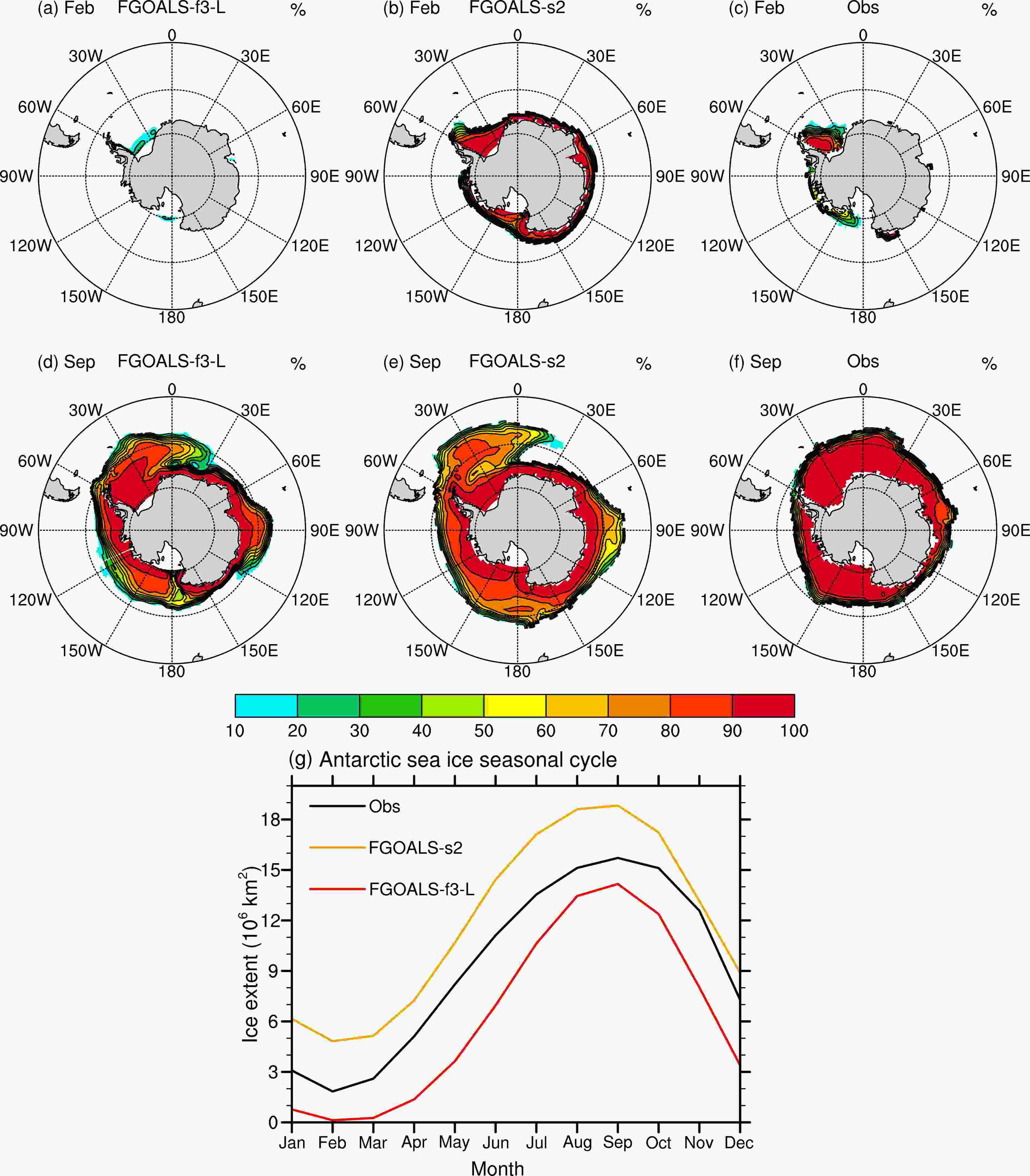 Figure11. Simulated sea ice concentrations (%) of (a, d) FGOALS-f3-L (1980–2014), (b, e) FGOALS-s2 (1980–2004) and (c, f) observations for Antarctica in (a–c) February and (d–f) September; and (g) the simulated seasonal cycle of sea ice extent (106 km2) in FGOALS-f3-L and FGOALS-s2, as well as the observation, for the Antarctic.
Comparing the FGOALS-f3-L and FGOALS-s2 simulations, the summer sea ice is overestimated in FGOALS-s2 but underestimated in FGOALS-f3-L in the Antarctic, which could be related to the weakened mixing and overestimated net heat fluxes there in the atmospheric model (He et al., 2019). For the winter Antarctic sea ice, the simulated spatial patterns in FGOALS-f3-L and FGOALS-s2 are similar, but the tail-like sea ice out of the Weddell Sea is remarkably reduced in FGOALS-f3-L, making the simulated sea ice distribution in this area more realistic. Additionally, for the seasonal cycle of sea ice extent (Fig. 11g), the bias changes from one of overestimation throughout the year in FGOALS-s2 to one of underestimation in FGOALS-f3-L, the causes of which need to be further analyzed.
Nevertheless, like most state-of-the-art coupled models (Johns et al., 2006; Griffies et al., 2011), obvious biases still exist in FGOALS-f3-L. The simulated global mean SST is colder than observed, and the most obvious SST biases are cold biases in the northwestern Pacific, northwestern Atlantic, GIN Sea and Barents Sea, and warm biases at the western and eastern oceanic boundaries and ACC areas. Most biases cannot be explained by simulated local net heat flux, except in the tropical oceans, but the simulated shortwave flux may contribute to these biases. The midlatitude cold biases could be related to the disadvantages of simulated western boundary currents and the strong anticyclonic curl of wind stresses. Besides, Huang et al. (2008) suggested that the lack of a wave mixing scheme could also contribute to midlatitude cold biases. The SSS is mainly underestimated globally; the freshwater biases in the western Pacific can be explained by excess precipitation; and the freshwater biases in the northwestern Atlantic can be explained by low evaporation. The simulated annual maximal MLDs mainly show deep biases in the subtropics and shallow biases at high latitudes. The subtropical deep biases could be related to the excess wind stresses and the high-latitude shallow biases could be related to the weak mixing. The abnormal distribution of MLD biases in the northern Atlantic could be related to sea ice biases. Regarding vertical structures, the main temperature biases are warm biases under 200 m, warm biases north of 60°N, and cold biases at high latitudes, which could be related to the weak mixing and water exchange between the Atlantic and Artic oceans. The main vertical salinity biases are freshwater biases in the upper 1000 m, except at 40°N and 60°S. AMOC observations are limited in time and space, but at 26.5°N—where the RAPID-AMOC data were collected—the simulated AMOC shows stronger northward (southward) transport in the upper (lower) ocean. The observations of MHTs from WOCE are also limited in several locations; however, in comparison, the simulated global MHT is smaller in the SH and similar in the NH, and the simulated Atlantic MHT is smaller north of 20°S and larger at 30°S.
As shown in the SIC distribution, the simulated Arctic winter sea ice is overestimated, while the Arctic summer sea ice and Antarctic (winter or summer) sea ice are underestimated. The overestimated biases of Arctic winter sea ice are mainly located from the Labrador Sea to the Barents Sea, which are the same locations as the aforementioned main biases of SST, SSS and MLDs, suggesting a close relationship between the sea ice biases and the other biases. The simulated Arctic sea ice extent is also overestimated in winter and underestimated in summer, showing an intense seasonal cycle, while the Antarctic sea ice extent is underestimated throughout the year.
Finally, all of the biases mentioned here highlight the disadvantages of FGOALS-f3-L, which must be noted by the developers and users of the model before applying it in scientific analyses and experiments. The most obvious biases in FGOALS-f3-L compared with FGOALS-s2 and other CMIP5 models are the cold biases in the northern Atlantic and the related overestimated sea ice, which are related to the weak mixing. Further in-depth studies need to be conducted on the specific physics and coupled interactions of the model to reveal the origins of the simulated biases, which will offer directions to improve the model in future versions.
Acknowledgements. This study was jointly supported by the Strategic Priority Research Program of the Chinese Academy of Sciences (Grant Nos. XDA19060102 and XDB42000000) and the National Natural Science Foundation of China (Grant Nos. 41530426, 91958201, and 41931183).
