HTML
--> --> -->Kellogg and Schilling (1951) conducted a study of stratospheric wind fields and first proposed a simple atmospheric circulation model that could reach up to an altitude of ~120 km. This model depicted the basic state of stratospheric circulation, and was later improved by other researchers (e.g., Murgatroyd, 1957; Batten, 1961; Kantor and Cole, 1964). Belmont and Dartt (1970) subsequently analyzed the characteristics of the monthly mean zonal winds at 40 and 50 km based on observational data for the time period 1961–1967. As a result of the temporal and spatial expansion of observational data, the stratospheric monthly mean zonal winds from 20 to 65 km were later analyzed for the time period 1961–1971 (Belmont et al., 1975). Clear seasonal variations and differences between the Northern and Southern Hemisphere were seen from the 11-year mean. For instance, during the Northern Hemisphere summer, easterly winds were dominant in the stratospheric wind fields above 20 km and enhanced significantly with height, whereas the westerly winds weakened significantly with height below 20 km, resulting in a weak wind layer at ~20 km with a wind speed < 10 m s?1. Lv et al. (2002) defined the concept of a zero wind layer based on the high air ball test, and the stratospheric quasi-zero wind layer (QZWL) was defined as the atmospheric layer in which the zonal wind direction reversed at ~20 km in the lower stratosphere, where the meridional wind speed and the full wind speeds were both very small.
The QZWL can provide a good meteorological environment for stratospheric airships and has therefore attracted much attention. Xiao et al. (2008) studied the temporal and spatial distribution of the stratospheric QZWL over China using ERA-40 reanalysis wind data, and found that the stratospheric QZWL over China mainly occurred in low latitudes in winter, in mid and high latitudes in summer, and in transitional areas in mid and low latitudes affected by the quasi-biennial oscillation (QBO). Tao et al. (2012) classified the stratospheric QZWL into two categories according to two different mechanisms of formation: The first type of stratospheric QZWL was a result of the transition between two phases of the QBO and mainly occurred in the tropical zone in winter. The second type of stratospheric QZWL was caused by the reversal of the meridional temperature gradient in the lower stratosphere and mainly existed in extratropical areas in summer and over the Pacific Ocean at mid and low latitudes (20°–40°N) in winter. Zhou et al. (2011) showed that the onset and withdrawal dates of the stratospheric QZWL were related to the stratospheric easterly winds.
Studies of the stratospheric QZWL have focused on the zonal distribution and statistical analysis of the stratospheric QZWL on interannual or seasonal time scales using data with a coarse spatial resolution (Belmont et al., 1975). There have been few studies that are able to help us recognize the fine structure and daily variation of the stratospheric QZWL. The flight time of stratospheric airships during testing is only few hours (Zhao et al., 2016), and the flight time of stratospheric airships with long-term targets is only one month (Yao et al., 2008). In addition, theory based on climatic reanalysis data that explain the zonal distribution of the stratospheric QZWL may not always apply to local and daily variations of the stratospheric QZWL. Therefore, to achieve long-duration flights and stable operation of stratospheric airships, it is necessary to determine the short-term variations of the stratospheric QZWL at higher temporal and spatial resolutions, given that existing research based on climatic reanalysis data has limited value for short-term flights of stratospheric airships. The control of stratospheric airships with artificial intelligence technology is inevitable and achievable in the near future. A better understanding of the fine structural features and short-term variations of the stratospheric QZWL is therefore required for better berthing, steering and other intelligent control of stratospheric airships. High-resolution data from radiosondes and numerical simulations with high resolutions are useful in achieving this goal.
We used high-resolution data from radiosondes in the Korla region to obtain the fine structure of the stratospheric QZWL. Information about the activities of mesoscale gravity waves in the lower stratosphere were based on previous studies (Yang et al., 2018), and the diagnostic equation for zonal winds was used to estimate the effect of the advection and wave terms on the stratospheric QZWL.
The stratospheric QZWL has not previously been analyzed quantitatively due to the lack of a specific definition. In this work, we classified the stratospheric QZWL as either a broadly or narrowly defined QZWL. A narrowly defined QZWL was defined as the weak wind layer between the altitudes of 18 and 22 km in which the minimum horizontal wind speed was < 2.5 m s?1, with reference to climate statistics (Yang., 2016), while a broadly defined QZWL was defined as the weak wind layer between the altitudes of 18 and 22 km in which the minimum horizontal wind speed was < 5 m s?1, with reference to engineering practices and observational data (Chen et al., 2018). Several other concepts related to the stratospheric QZWL were also defined to depict the stratospheric QZWL. The thickness of the narrowly (broadly) defined QZWL was the difference between the altitude (18–22 km) at which the contour of the horizontal wind speed with a value of 2.5 m s?1 (5 m s?1) occurred for the first and second time. The height of the narrowly (broadly) defined lower QZWL was the altitude (18–22 km) at which the contour of the horizontal wind speed with a value of 2.5 m s?1 (5 m s?1) occurred for the first time from bottom to top. The height of the narrowly (broadly) defined higher QZWL was the altitude (18–22 km) at which the contour of the horizontal wind speed with a value of 2.5 m s?1 (5 m s?1) occurred for the second time from bottom to top.
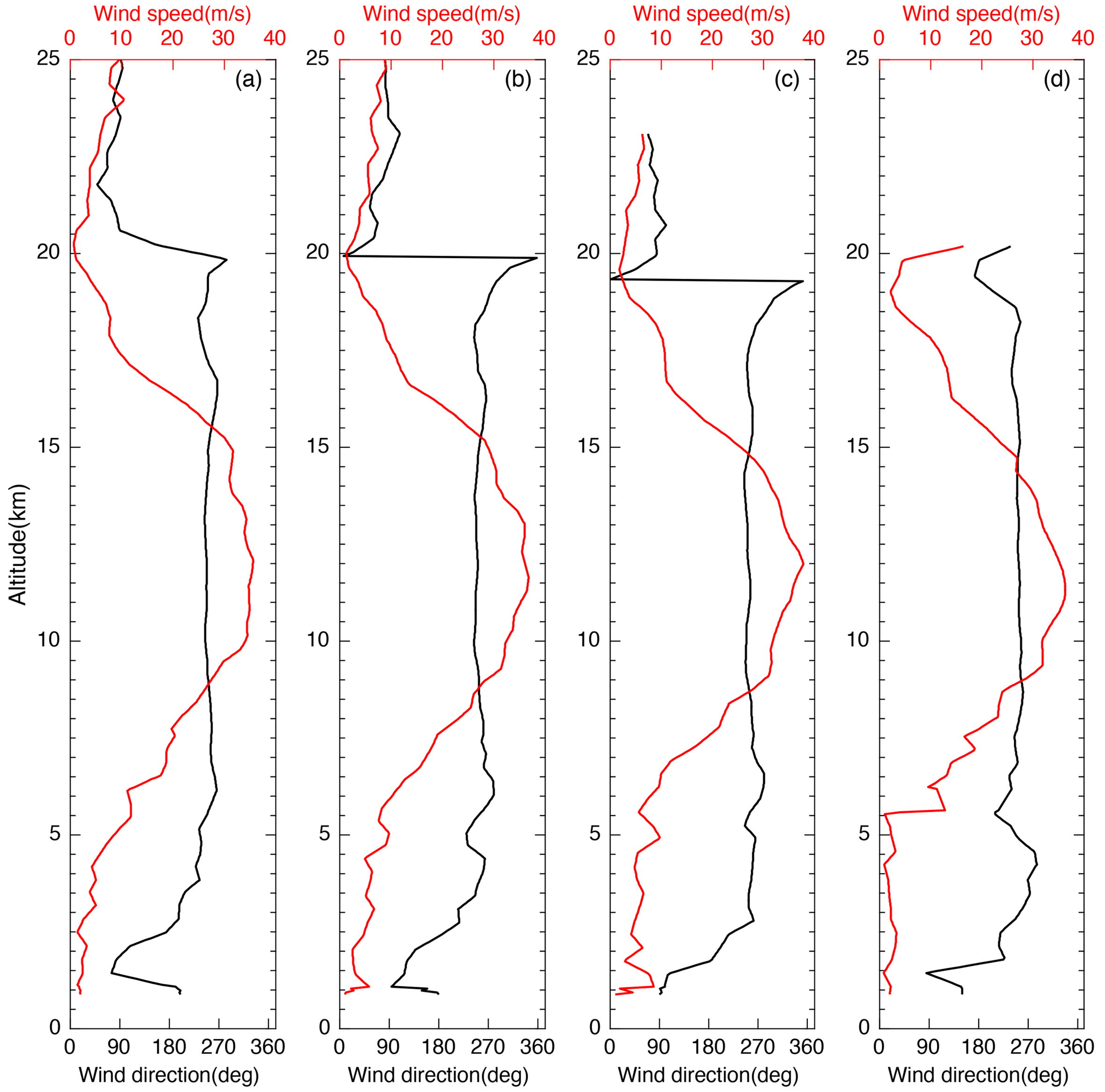 Figure1. Observed horizontal wind speed (red) and wind direction (black) at (a) 1800 UTC and (b) 2000 UTC 18 August 2016, and (c) 0000 UTC and (d) 0300 UTC 19 August 2016.
At 1800 UTC, the wind direction changed with height in a counterclockwise direction (Fig. 1a). The wind direction changed from westerly at 19.9 km to southerly at 20.2 km and then to easterly at 20.6 km, remaining easterly above this height. The maximum change in wind direction exceeded 180°. At 2000 UTC, by contrast, the wind direction in the QZWL region changed in a clockwise direction with height (Fig. 1b). The wind changed from westerly at 18.9 km to northerly at 19.9 km and then to easterly at 21.1 km, remaining easterly above this height. The maximum change in wind direction exceeded 180°. Similarly, at 0000 UTC, the wind direction in the QZWL region changed in a clockwise direction with height (Fig. 1c). The wind shifted from westerly at 18.2 km to northerly at 19.3 km and then to easterly at 20.1 km, remaining easterly above this height. The maximum change in wind direction also exceeded 180°. At 0300 UTC, the wind direction in the QZWL region changed in a counterclockwise direction with height (Fig. 1d). The wind shifted from westerly at 18.5 km to southerly at 19.5 km and then to westerly above 19.5 km; the maximum change in wind direction was only 90°.
Figure 2 shows the profile of the zonal and meridional winds during the four measurements. At 1800 UTC, both the zonal and meridional winds increased with increasing altitude below 5 km (Fig. 2a). The difference between the zonal and meridional wind speeds, which were both < 10 m s?1, was not large and both wind speeds increased rapidly at 5–12 km. The maximum meridional wind was ~18 m s?1 at 12–13 km, whereas the maximum zonal wind exceeded 30 m s?1 at 12 km. The zonal wind decreased rapidly above 12 km, reaching 0 m s?1 at ~20 km. The zonal wind shifted to easterly and increased with increasing altitude above 20 km. The meridional wind decreased rapidly above 13 km and reached 0 m s?1 at ~16.5 km. The meridional wind speed remained around 0 m s?1 above 16.5 km. The vertical structures of the zonal and meridional winds at 2000 (Fig. 2b) and 0000 (Fig. 2c) UTC were similar to those observed at 1800 UTC. At 0300 UTC, the winds differed from the trends observed during the previous three measurements (Fig. 2d). The meridional wind increased with increasing altitude after reaching a minimum at 18.5 km. The zonal wind increased with increasing altitude after reaching a minimum at 19.5 km. In the QZWL region, the zonal wind shifted from westerly to easterly, while the meridional wind speed was low and did not vary much from 0 m s?1.
 Figure2. Observed zonal winds (red) and meridional winds (blue) at (a) 1800 UTC and (b) 2000 UTC 18 August 2016, and (c) 0000 UTC and (d) 0300 UTC 19 August 2016.
The radiosonde profiles of temperature and humidity (Fig. 3) showed that the tropopause defined using the coldest point was 17–18 km, with a temperature of about ?68°C. The QZWL was located 1–2 km above the tropopause. The relative humidity decreased to a minimum value at 8–9 km during all four measurements. At 1800 and 2000 UTC, the relative humidity above 8 km was stabilized at ~10% and ~30%, respectively. At 0000 and 0300 UTC, the relative humidity above 9 km was stabilized at ~15% and ~5%, respectively.
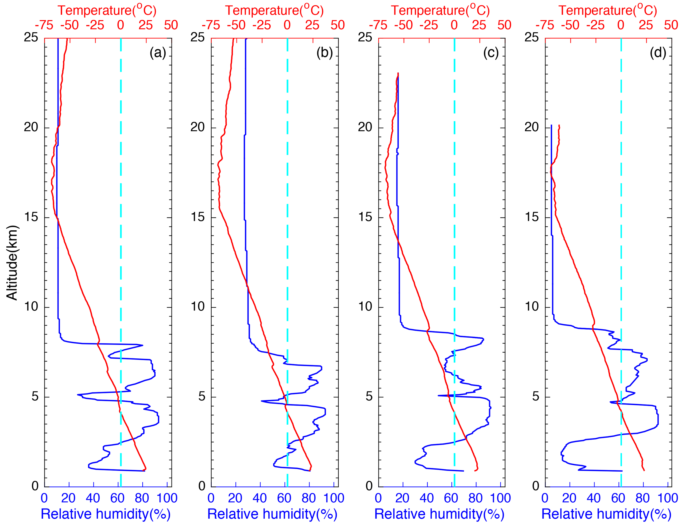 Figure3. Temperature (red) and relative humidity (blue) at (a) 1800 UTC and (b) 2000 UTC 18 August 2016, and (c) 0000 UTC and (d) 0300 UTC 19 August 2016.
 Figure4. Geopotential height (solid black lines; units: dagpm) and temperature (dashed red lines; units: K) at 500 hPa at (a) 1800 UTC 18 August 2016 and (b) 0000 UTC, (c) 0600 UTC and (d) 1200 UTC 19 August 2016.
At 1800 UTC, a stable ridge was observed at 100 hPa (Fig. 5) to the west of the Ural Mountains over the Caspian Sea. A trough to the east of the Aral Sea continuously developed southward and the South Asian high was maintained over the eastern Tibetan Plateau. Two isolated high-pressure centers had appeared by 0000 UTC as a result of the continuously southward-developing Central Asian trough. A high-pressure center emerged over the south of the Caspian Sea. The South Asian high over the eastern Tibetan Plateau moved eastward. The Central Asian trough weakened at 0600 UTC and the South Asian high extended westward, strengthening further at 1200 UTC.
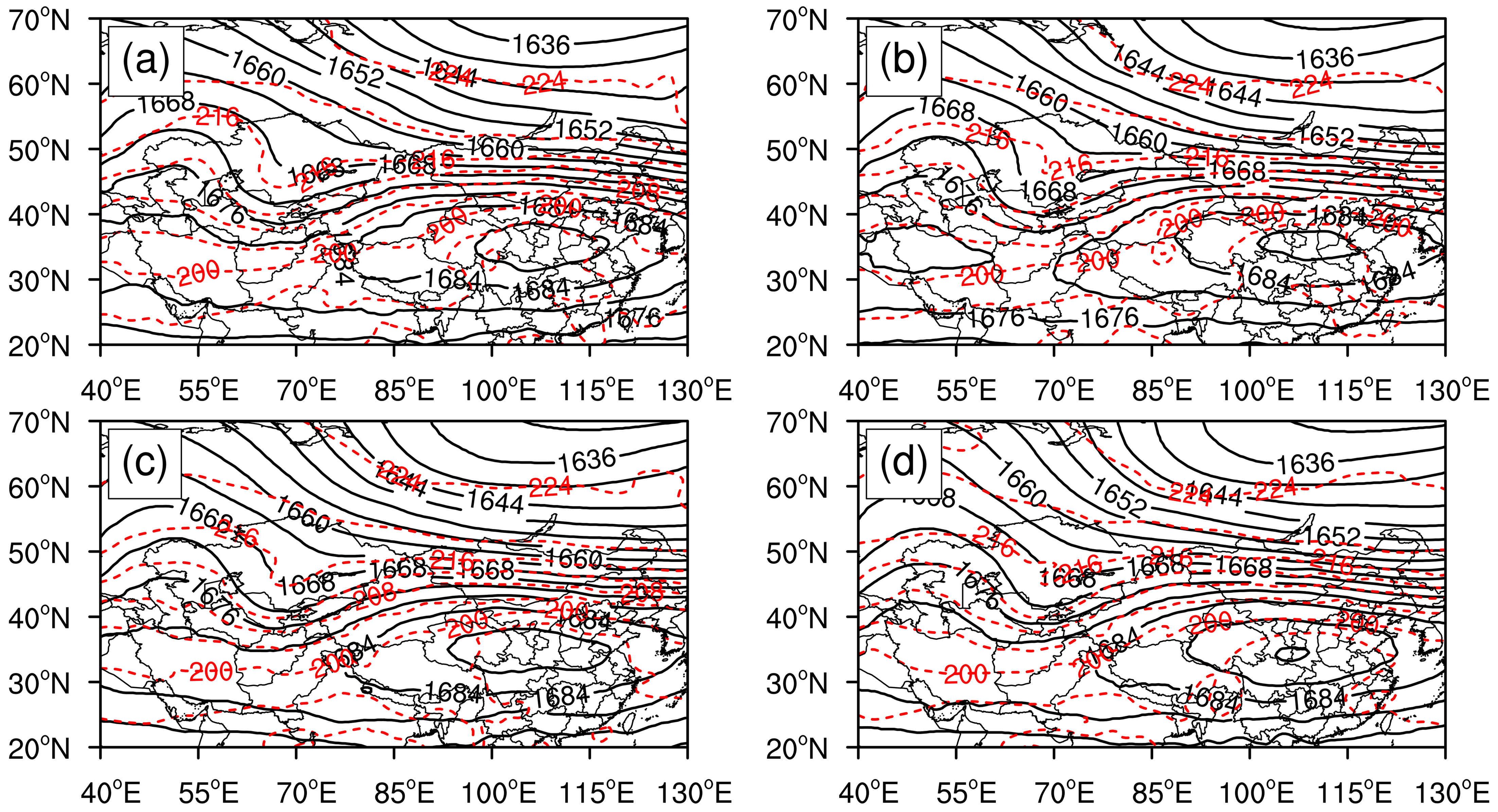 Figure5. . Geopotential height (solid black lines; units: dagpm) and temperature (dashed red lines; units: K) at 100 hPa at (a) 1800 UTC 18 August 2016 and (b) 0000 UTC, (c) 0600 UTC and (d) 1200 UTC 19 August 2016.
Analysis of the weather systems showed that the highs were stable and remained to the east of the Tibetan Plateau from 1800 to 1200 UTC the following day. The highs inclined westward with height and Korla was situated in the northwest of the highs. When the wind in the QZWL region shifted from westerly to easterly with height at 1800 UTC, the South Asian high was relatively strong and the Central Asian trough was relatively weak. However, when the wind in the QZWL region shifted from westerly to easterly with height at 0000 UTC, the South Asian high became weaker and the Central Asian trough became stronger. Strengthening (weakening) of the Central Asian trough was accompanied by weakening (strengthening) of the South Asian high and the relationship between the Central Asian trough and the South Asian high was related to the transformation mode of the wind direction in the QZWL region. The strengthening of the South Asian high and the weakening of the Central Asian trough resulted in the wind over the observation site becoming more affected by the South Asian high, which caused the wind to shift in a clockwise direction with height. By contrast, the weakening of the South Asian high and the strengthening of the Central Asian trough resulted in the wind over the observation site becoming more affected by the Central Asian trough, which caused the wind to shift in a counterclockwise direction with height.
5.1. Model description
The Weather Research and Forecasting (WRF) model, version 3.7.1, was used to simulate the stratospheric winds in a single domain with 539 × 384 grid points in the north–south and east–west directions, respectively, 100 vertical levels with a model top of 5 hPa, and a horizontal grid spacing of 3 km. The simulation was performed over a period of 48 h from 0600 UTC 18 August 2016 to 0600 UTC 19 August 2016. The main parameterizations used in the model were as follows: a microphysics scheme with ice, snow and graupel processes suitable for high-resolution simulation (Thompson microphysical scheme); a boundary scheme from the asymmetrical convective model with a non-local upward mixing and local downward mixing closure scheme (ACM2); a two-layer scheme from the Pleim–Xiu land surface model with vegetation and sub-grid tiling (PX LSM); and a longwave radiation scheme from the Rapid Radiative Transfer Model (RRTM). The model was set up to provide an output every 10 min. The simulation area and topographic distribution are presented in Fig. 6.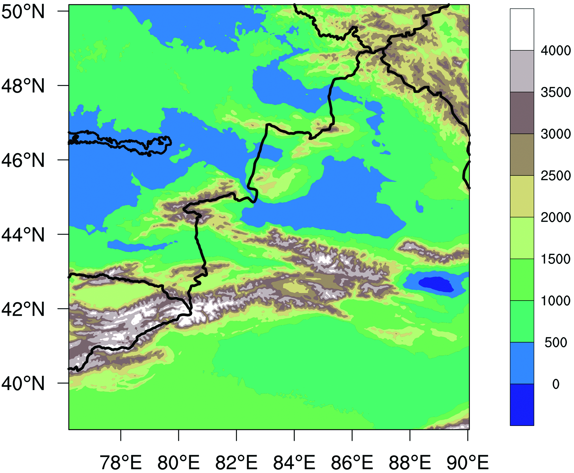 Figure6. Terrain height (units: m) in the numerical simulation domain.
2
5.2. Simulation of winds over Korla
A comparison of the radiosonde data and model-simulated vertical distributions of horizontal wind speed showed good agreement (Fig. 7), particularly in the QZWL region of the lower stratosphere, with a minimum wind speed at ~20 km. At 1800 UTC, the minimum wind speed in the simulation at 20 km was ~2.5 m s?1 (Fig. 7a), about 2 m s?1 greater than the observed speed. At 2000 UTC, the minimum wind speed in the simulation at 20 km was ~1.5 m s?1 (Fig. 7b), consistent with the observations. At 0000 UTC, the minimum wind speed in the simulation at 20 km was ~0.5 m s?1 (Fig. 7c), about 2 m s?1 lower than the observations; however, the simulated minimum wind speed occurred at a higher altitude than the observed result. At 0300 UTC, the minimum wind speed in the simulation at 20 km was ~1.5 m s?1 (Fig. 7d), consistent with the observations; however, the simulated minimum wind speed also occurred at a higher altitude than the observed result.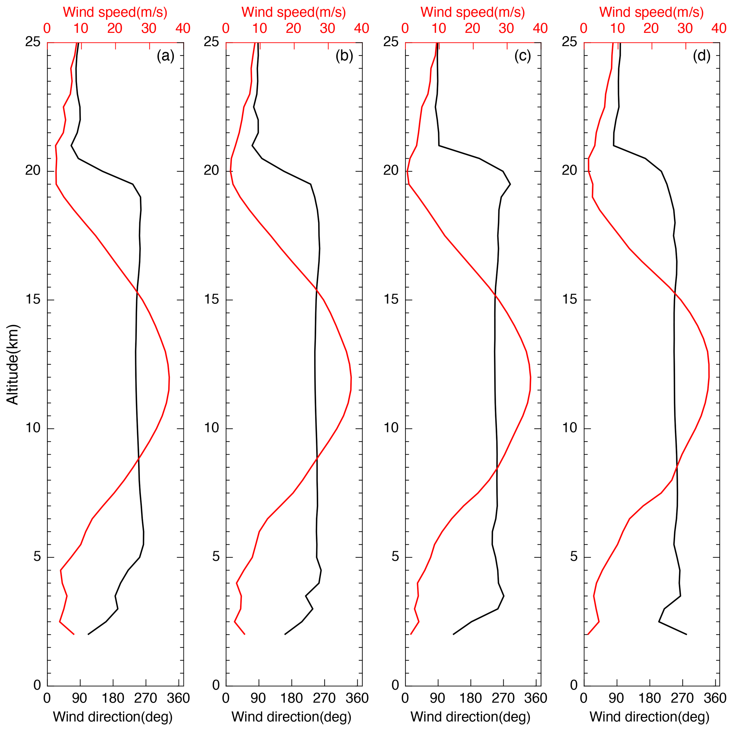 Figure7. Simulated horizontal wind speed (red) and wind direction (black) at (a) 1800 UTC and (b) 2000 UTC 18 August 2016, and (c) 0000 UTC and (d) 0300 UTC 19 August 2016.
The change in wind direction was simulated to occur at an altitude of ~20 km for the four time points. At 1800 UTC, the simulated wind direction shifted from westerly to easterly with height (Fig. 7a), consistent with the observations. Also consistent with the observations, the wind direction shifted from westerly to easterly in a counterclockwise direction with height and the maximum change in wind direction in the QZWL region was about 180°. At 2000 UTC, the simulated wind direction shifted from westerly to easterly in a counterclockwise direction with height (Fig. 7b), contrary to the observations. The simulated wind direction at 0000 UTC shifted from westerly to easterly in a clockwise direction with height (Fig. 7c), the same as the observations. At 0300 UTC, the simulated wind direction shifted from westerly to easterly in a counterclockwise direction with height and the maximum change in wind direction in the QZWL region was about 180° (Fig. 7d); however, the maximum change in the observations was only 90°.
Figure 8 presents the evolution of the horizontal wind speed and direction with height over a 24-h period from 0600 UTC 18 August to 0600 UTC 19 August 2016. The narrowly defined QZWL mainly appeared between 18.9 and 21.2 km and therefore the maximum thickness of the narrowly defined QZWL was 2.3 km. The broadly defined QZWL mainly appeared between 18.8 and 23.1 km, which meant that the maximum thickness of the broadly defined QZWL was about 4.3 km. The height of the narrowly defined higher QZWL and the height of the narrowly defined lower QZWL both varied rapidly with time, whereas the height of the broadly defined lower QZWL varied slowly with time. The height of the broadly defined higher QZWL varied dramatically with time, especially from 1200 to 1800 UTC 18 August 2016, when the height of the broadly defined higher QZWL decreased rapidly with time. The height of both the broadly and narrowly defined higher QZWL decreased fastest with time from 1700 to 2000 UTC 18 August 2016, during which time the height of the broadly defined higher QZWL decreased sharply to 20.8 km from 1700 to 1800 UTC 18 August 2016 and the narrowly defined QZWL was interrupted from 1800 to 1900 UTC 18 August 2016. After a short interruption, the narrowly defined QZWL recovered quickly and the thickness of both the broadly and narrowly defined QZWL was relatively stable. Based on classical atmospheric dynamics theory, the change in the vertical gradient of zonal winds is largely determined by the change in the meridional gradient of the temperature field, which, in turn, is determined by the large-scale circulation and synoptic-eddy structures and can result in the formation of the QZWL. However, the flow under rapid changes is likely ageostrophic and thus does not satisfy the thermal wind balance.
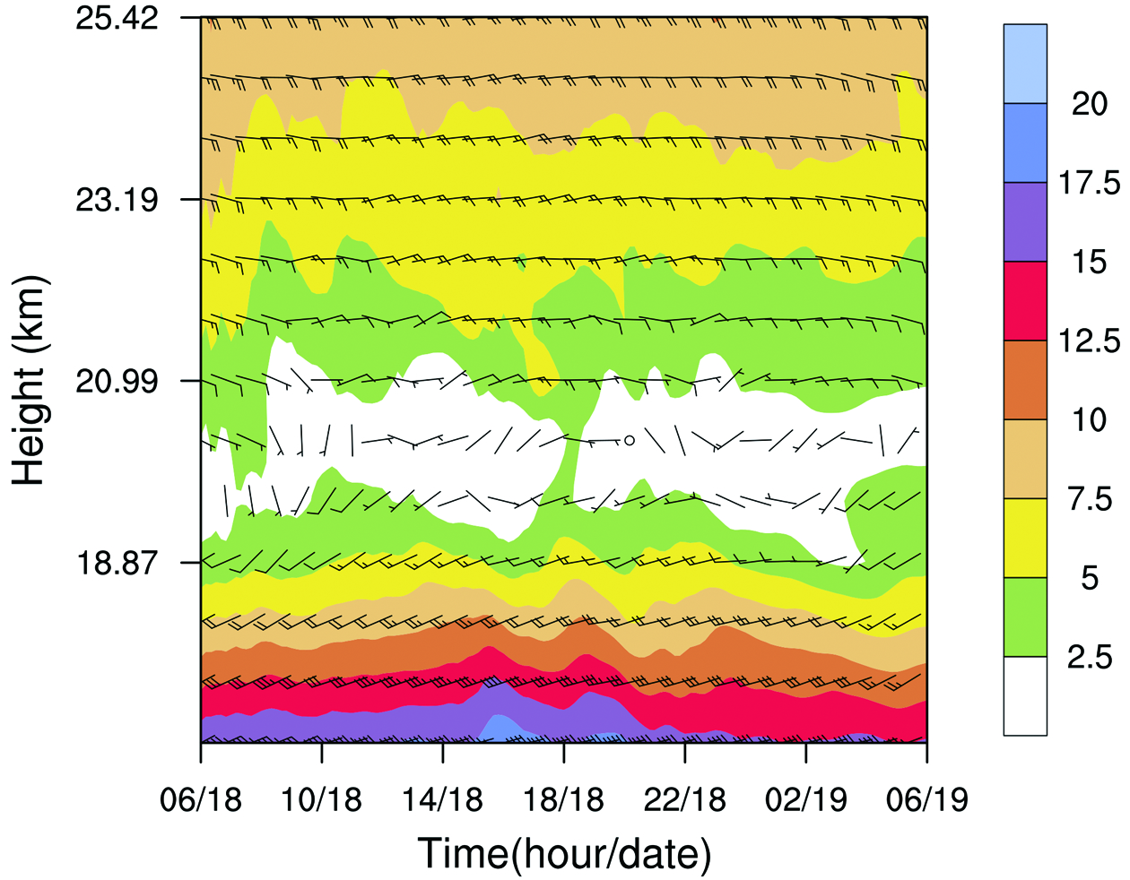 Figure8. Evolution of horizontal wind speed (units: m s?1) and wind direction over Korla from 0600 UTC 18 to 0600 UTC 19 August 2016.
2
5.3. Diagnosis of the zonal wind
The horizontal wind speed was mainly affected by the zonal wind, especially in the QZWL region. The zonal wind was significantly greater than the meridional wind below 20 km and the meridional wind approached 0 m s?1 above 20 km. The changes in the winds in the QZWL region were predominantly determined by the zonal wind and therefore the zonal wind was used to analyze the forcing factors affecting the height and thickness of the stratospheric QZWL.Kinoshita and Sato (2013a, b) derived the form of three-dimensional Eliassen–Palm flux suitable for mesoscale gravity waves based on the basic equations of atmospheric motion. These equations could be used to diagnose the forcing effect of mesoscale waves on the mean flow. The residual circulations defined by Kinoshita and Sato (2013a, b) were improved to obtain a form of three-dimensional Eliassen–Palm flux suitable for analysis under non-hydrostatic equilibrium (Liu et al., 2019):
where the variable with the signal of “-” represents the time mean and the variable with the signal of “ ′ ” represents the deviation from the time mean; x, y, z represent horizontal and vertical component of physical quantity; t is time; u, v and w are the zonal, meridional and vertical velocities, respectively; p is the pressure; ρ is the air density; f is the Coriolis parameter;


where θ is the potential temperature; g is gravitational acceleration; and


We define


Although the analyzed QZWL at Korla is local, it may well be part of a large-scale phenomenon as well as being influenced by ageostrophic, mesoscale disturbances such as gravity waves. If the former dominates, the changes in zonal winds are largely determined by the changes in the meridional gradient of the temperature field, which is, in turn, determined by the large-scale circulation and synoptic-eddy structures. To evaluate the ageostrophic effect, a Barnes filter was used to filter out the ageostrophic components. The expressions of the modified Barnes filter are as follows (Zou et al., 2018):
where D(x, y) is the variable (e.g. geopotential height) simulated by the WRF model, D0(x, y) is the initial filter value of D(x, y), D1(x, y) is the final filter value of D(x, y), M is the grid number within an influence range of the grid point (x, y),


where θ and φ are the longitude and latitude, respectively, of grid point (x, y) and


A low-pass filter was applied to extract the large-scale background flow with horizontal wavelengths over 300 km (Zhang, 2004; Zhang et al., 2007; Wei and Zhang, 2015; Kim et al., 2016). The response function is shown in Fig. 9, in which the response with C = 2500 and G = 0.35 is close to 0.8 when the wavelength is 300 km.
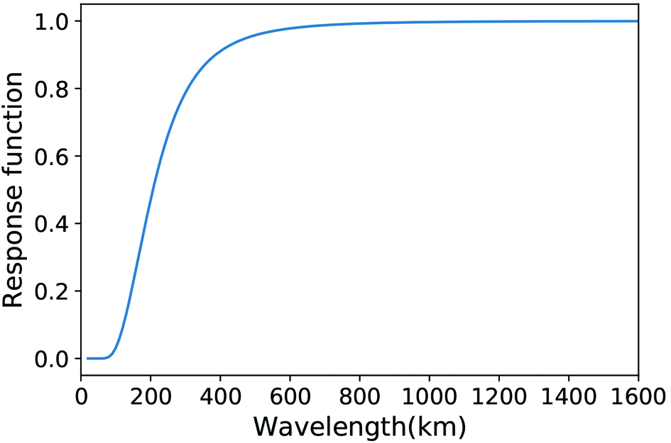 Figure9. Response function of the Barnes filter when C = 2500 and G = 0.35.
Figure 10 shows the influence of these forcing factors on the zonal winds at 1700 and 1800 UTC 18 August 2016. Comparing the two times, the advection term had the most important role among the three forcing terms. The pressure gradient term was the weakest forcing term and was two orders of magnitude smaller than the other two forcing terms, meaning that it had a very limited forcing effect on the zonal wind. The influence of the wave term was weaker than that of the advection term, but was significant in some regions over the observation site. For the advection term, negative forcing was dominant at ~21 km, whereas positive forcing was remarkable below 20 km over the observation site at 1700 UTC. Negative forcing was also remarkable for the wave term at ~21 km over the observation site at 1700 UTC and its forcing effect was comparable with that of the advection term. The negative forcing of the advection and wave terms together caused an increase in easterly winds at 21 km (Fig. 10). The forcing of the advection term on the horizontal wind became positive at ~21 km over the observation site at 1800 UTC, whereas forcing of the wave term on the zonal wind became very weak. This meant that the advection term began to force the easterly winds to decrease and the effect of the wave term became very small. As a result, the horizontal wind speed began to increase after 1800 UTC. The effect of the advection term was always strong, explaining the maintenance of the ridge–trough pattern shown in Figs. 4 and 5.
 Figure10. Diagnosed results along 41.82°N at (a–c) 1700 UTC and (d–f) 1800 UTC 18 August 2016, based on the diagnostic equation of zonal wind: (a, d) advection term (equ2) (units: 10?4 m2 s?3); (b, e) pressure gradient term (equ3) (units: 10?6 m2 s?3); and (c, f) wave term (equ4) (units: 10?4 m2 s?3). The vertical dashed black line indicates the position of 86.77°E.
Figure 10 shows that the advection and wave terms were the main forcing factors for the zonal wind. The two terms were further divided into different sub-items. The advection term (equ2), where equ2 =


 Figure11. Diagnosed results along 41.82°N at (a–d) 1700 and (e–h) 1800 18 August 2016, based on the diagnostic equation of zonal wind: (a, e) equ21 term (units: 10?5 m s?2); (b, f) equ22 term (units: 10?5 m s?2); (c, g) equ23 term (units: 10?5 m s?2); and (d, h) equ24 term (units: 10?4 m s?2). The vertical dashed black line indicates the position of 86.77°E.
The wave term (equ4) was also divided into three sub-items: equ41 =


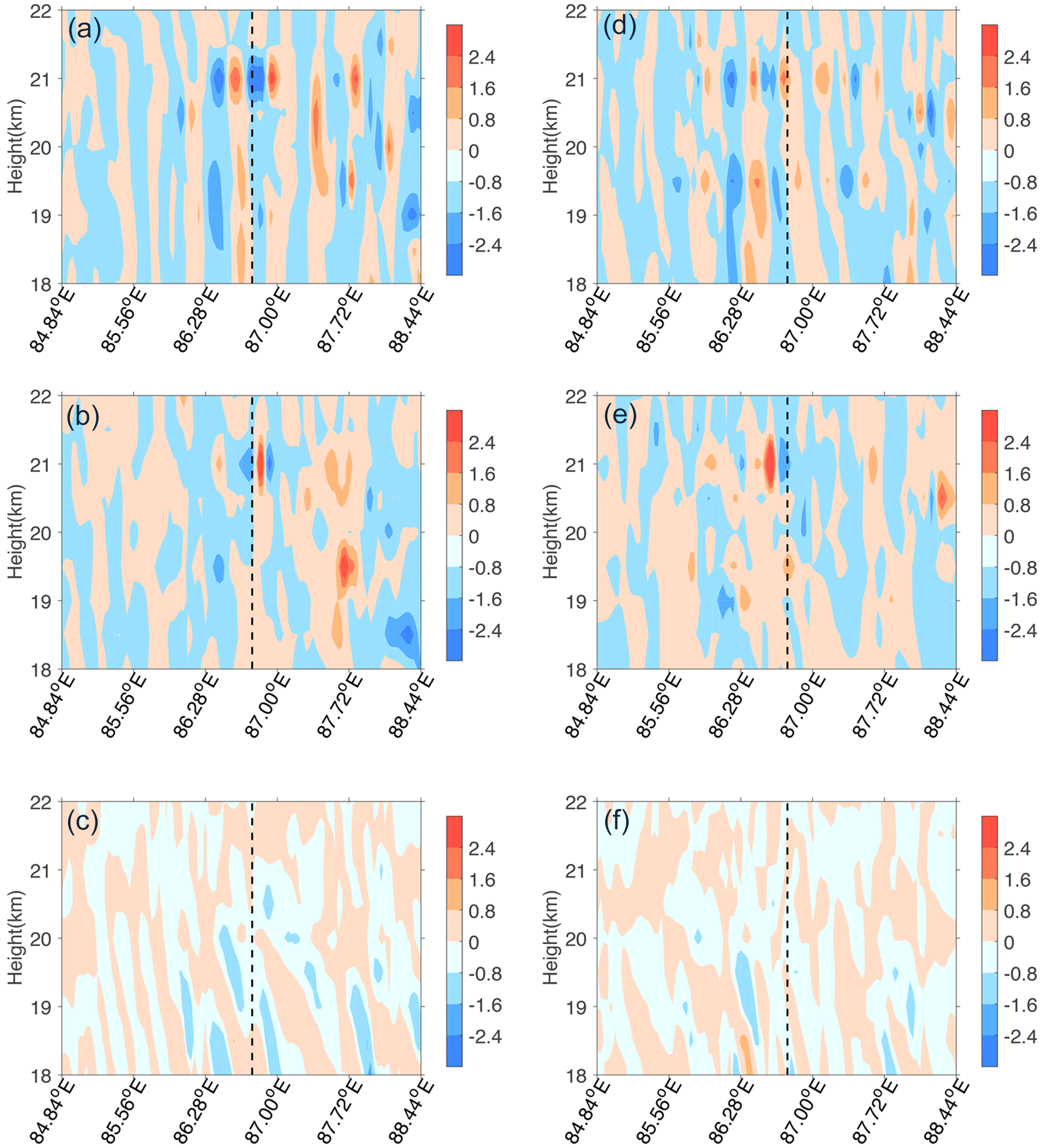 Figure12. Diagnosed results along 41.82°N at (a–c) 1700 UTC and (d–f) 1800 UTC 18 August 2016, based on the diagnostic equation of zonal wind: (a, d) equ41 term (units: 10?4 m s?2); (b, e) equ42 term (units: 10?4 m s?2); and (c, f) equ43 term (units: 10?4 m s?2). The vertical dashed black line indicates the position of 86.77°E.
Numerical simulation of the wind speed and direction over the observation site effectively captured the structural characteristics of the change in the stratospheric QZWL with time and height. The narrowly (broadly) defined QZWL appeared at 18.9–21.2 km (18.8–23.1 km), with the thickness varying from 0 to 2 km (2 to 5 km). The simulation was able to reproduce the minimum wind speed in the QZWL region and the height at which the wind direction reversed.
The analysis based on the diagnostic equation of the zonal wind further clarified the influence of the different forcing factors on the zonal wind in the QZWL region. The advection term was the dominant factor and the pressure gradient term was the weakest factor. The wave term also played a significant part at some times and in some locations and, together with the advection term, interrupted the stratospheric QZWL. The residual term, the zonal transportation term and the meridional transportation term were the main factors in the advection and wave term, respectively.
The fine structure and time-varying characteristics of the stratospheric QZWL were analyzed from the observational data and the ability of the WRF model to simulate the structural features of the stratospheric QZWL was tested. The model simulated the horizontal wind speed well, but the simulations of the reversal of wind direction in the QZWL region need to be improved. Analysis of the results showed the indispensable influence of the wave term in the QZWL region, although additional research is required to strengthen our understanding of the stratospheric QZWL.
Acknowledgments. This work was supported by the Strategic Priority Research Program of the Chinese Academy of Sciences (Grant No. XDA17010105). The GFS data used in this paper are available at http://nomads.ncdc.noaa.gov/data/gfs4.
