HTML
--> --> -->The results of OMIP-1 and OMIP-2 from 11 state-of-the-art global low-resolution ocean–sea-ice models were evaluated by Tsujino et al. (2020). Some improvements to key features were identified from the comparison, such as the attenuation of the warming biases off the eastern coast of the Pacific Ocean, as well the reproduction of the observed global warming and warming hiatus in the sea surface temperature (SST). However, some common model biases still persist, indicating errors in representing important processes or biases in the surface forcing. Among the possible causes, the horizontal resolution of the model is considered to be one of the important factors, particularly for the biases in eddy-rich regions, western boundary currents, and narrow straits. Therefore, additional OMIP-2 experiments using global eddy-resolving ocean–sea-ice models were proposed and compared by Chassignet et al. (2020) to identify the robust improvements of ocean–sea-ice simulation by refining the model resolution from 100 km to 10 km.
Under the framework of this resolution-related comparison, four ocean modeling groups have conducted and submitted a pair of experiments: 100 km and 10 km versions of the model forced by the JRA55-do dataset for only one cycle (1958–2018). The experiments of the coarse resolution are just the same as the first cycle of OMIP-2 in Tsujino et al. (2020). The Chinese Academy of Science, State Key Laboratory of Numerical Modeling for Atmospheric Sciences and Geophysical Fluid Dynamics/Institute of Atmospheric Physics (LASG/IAP) Climate system Ocean Model, version 3 (CAS-LICOM3) is one of the models that has participated in the comparisons, which was developed based on the previous version, CAS-LICOM2 (Liu et al., 2012). CAS-LICOM3 is also the ocean component of FGOALS3, participating in CMIP6. The eddy-resolving simulation of CAS-LICOM3 for OMIP-2 (hereafter called CAS-LICOM3_High) was finished in November 2019 and the data submitted to the Earth System Grid Federation (ESGF) data server (
The organization of the paper is as follows. In section 2, we describe the ocean model, the experiment design, and the methods used here. Section 3 presents the basic technical validation of CAS-LICOM3_High. In this section, firstly, the temporal evolution of SST, sea surface salinity (SSS), Atlantic Meridional Overturning Circulation (AMOC), kinetic energy (KE), and upper-ocean temperature are presented for examining the trends and variabilities of the simulation. Secondly, the simulated spatial pattern and standard deviation (STD) of sea surface height (SSH) and SST are validated by splitting the large-scale signal and mesoscale eddies. Thirdly, the ocean surface currents are provided for showing the major currents, such as the western boundary currents and Antarctic Circumpolar Current (ACC). Finally, the North Equatorial Undercurrent (NEUC) is selected to evaluate this dataset, because it is a good indicator to examine the long-term and high-resolution simulation (Li et al., 2018). In section 4, the data record is described. Section 5 provides usage notes.
2.1. Introduction to the model
CAS-LICOM is a global ocean general circulation model developed by LASG/IAP of the Chinese Academy of Sciences (Zhang and Liang, 1989; Liu et al., 2004, 2012; Yu et al., 2018). CAS-LICOM3 is an ocean general circulation model with a free sea surface and Arakawa B grid, and uses the primitive equations with Boussinesq and hydrostatic approximations. It has been extensively upgraded since CAS-LICOM2. First, the coordinates of the dynamical core have been replaced by arbitrary orthogonal curvilinear coordinates (Yu et al., 2018). Therefore, the tripolar grid from Murray (1996) can be applied in CAS-LICOM3, with two North Poles, on the Eurasian (55°N, 95°E) and North American (55°N, 85°W) continents, respectively.Second, the coupler was updated from NCAR flux coupler 6 to coupler 7 when the ocean component was coupled with the Community Ice Code, version 4 (CICE4). Also, it has been proved to be helpful for the high-resolution coupling (Lin et al., 2016).
Third, the central difference scheme is used in the momentum equations and the Leapfrog format with an Asselin filter is used for the time integration of the momentum equations. Additionally, the two-step preserving shape advection scheme (Yu, 1994; Xiao, 2006) and implicit vertical viscosity/diffusivity (Yu et al., 2018) were adopted for the tracer equations.
Fourth, with regard to the physical processes, the St. Laurent et al. (2002) internal tidal mixing scheme has been introduced into CAS-LICOM3 (Yu et al., 2017). The vertical viscosity and diffusion coefficients in the mixed layer are computed by the scheme of Canuto et al. (2001, 2002), with background values of 2 × 10?6 m2 s?1 and upper limit of 2 × 10?2 m2 s?1. Besides, the chlorophyll-a dependent solar penetration of Ohlmann (2003) introduced by Lin et al. (2007) was also implemented in CAS-LICOM3.
2
2.2. High-resolution experiment design
The eddy-resolving simulation of CAS-LICOM3 (CAS-LICOM3_High) is forced by JRA55-do data (Tsujino et al., 2018), which were developed based on the JRA-55 product (Kobayashi et al., 2015). The temporal resolution of JRA55-do is 3-h and the horizontal resolution is 0.5625°. The atmospheric state variables and radiative fluxes are employed to compute the net surface flux into the ocean–sea-ice system in JRA55-do data, which included the air temperature at 10 m, the air density at 10 m, the relative humidity at 10 m, the surface wind vectors at 10 m, the sea surface pressure, the surface downward and upward shortwave flux, and the surface downward longwave flux (here, flux into the ocean is called “downward”). The turbulence heat and momentum fluxes of JRA55-do data have been computed using the bulk formula of Large and Yeager (2004). In the formula, the relative 10 m winds are employed and they are obtained by subtracting full ocean currents from the 10 m winds. The freshwater flux includes the precipitation (snow and rainfall) from JRA-55, as well as the continental runoff, which incorporates the runoff of ice sheets and glaciers from Greenland and Antarctica. The simulation is forced every 6 hours, even though the JRA55-do data are three-hourly, and integrated for 61 years from 1958 to 2018.The experiment follows the OMIP-2 protocol, with the initial condition of the temperature and salinity from observation and a state of rest. The initial values in this study are different from the standard OMIP-2 experiment; they are the temperature and salinity on 1 January 2014 from the Mercator Ocean analysis (Lellouche et al., 2018; Artana et al., 2019), not the World Ocean Atlas (Antonov et al., 2006, 2010; Locarnini et al, 2006, 2010). Meanwhile, the surface salinity is restored to the monthly Polar Science Center Hydrographic Climatology, version 3 (PHC3.0; Steele et al., 2001) over the entire domain with a salinity piston velocity of 50 m (4 yr)?1 [plus 50 m (30 d)?1 for the sea ice regions].
The horizontal grid contains 3600 × 2302 points with a resolution of approximately 1/10°, which is 11 km zonally and varies from 11 km at the equator to 8 km in midlatitudes and 2.7 km around the Antarctic. The higher resolution of CAS-LICOM3_High than the forcing data may imply that eddy-resolving activities come from the internally generated variability. The

2
2.3. Methods
To avoid the interference of the long-term trend and seasonal cycle when analyzing the temporal variations, the least-squares linear trend is first removed. Then, the de-seasonalized method is applied. The de-seasonalized method here means the removal of the climatological monthly mean from the detrended time series.The STD here is calculated after removing the least-squares linear trend and the seasonal cycle. Also, the data from CAS-LICOM3_High are interpolated into a 25-km resolution when comparing with the observations or reanalysis data.
The spatial correlation coefficient calculated in this study is the Pearson product-moment coefficient of linear correlation between two datasets. For the Pearson correlation coefficient, the linear change of the two variables will not change the value of Pearson correlation. That is, high correlation does not mean two variables are exactly the same; rather, that they have the same spatial gradient.
The root-mean-square error (RMSE) of SST calculated in this study is also based on the model data interpolated to the observation grid. The formula is:
where Ai stands for the area of each grid cell; and SSTmodel and SSTobs are the simulated and observed SST, respectively.
A spatial filter method is used here, which is adopted from Bryan et al. (2010) and Lin et al. (2019), to extract the oceanic mesoscale signal. First, a filter box with 3° of longitude and 3° of latitude is used for monthly mean data to obtain the box-mean value as the lowpass-filtered value. The value is considered as the large-scale signal. Second, the STDs of both daily SST and the lowpass-filtered monthly SST are calculated. Third, the difference between those two STDs is used to reflect the role of the mesoscale signal. In that way, the impact of the interannual variability of large-scale signals can be removed.
The eddy kinetic energy (EKE) computed here is the square of the temporal anomaly of the velocity (


where


3.1. Temporal evolution
The temporal evolutions of the annual mean globally averaged SST, SSS, AMOC, KE and temperature anomaly over the Ni?o3.4 index region from CAS-LICOM3_High are evaluated against the observation, reanalysis and the low-resolution experiment (CAS-LICOM3_Low; see details in Appendix A) (Fig. 1). The temporal evolution of the annual globally averaged SST is captured well by CAS-LICOM3_High (Fig. 1a). Here, three validated datasets have been applied, including the Extended Reconstructed SST, version 5 (ERSST.v5; resolution of 2°; Huang et al., 2017), Optimum Interpolation Sea Surface Temperature, version 2 (OISSTv2; resolution of 1/4°; Banzon et al., 2016; Reynolds et al., 2007), and SST from IAP (IAP_T; resolution of 1°; Cheng et al., 2015). An obvious warming trend of about 0.11°C (10 yr)?1 can be seen during 1958–2018, and 0.13°C (10 yr)?1 during 1982–2018, in CAS-LICOM3_High. The trends during the two periods are larger than those from ERSST.v5 and slightly smaller than those from OISSTv2. Compared with OISSTv2, the trends in CAS-LICOM3_High are better than those in CAS-LICOM3_Low, which may be related to the better simulation of both large-scale currents and mesoscale eddies in CAS-LICOM3_High. The STDs range from 0.06°C to 0.08°C for all simulations and observations, and the correlations are all higher than 0.9, as listed in Table 1. This suggests both the magnitude and phase of interannual–decadal variability in CAS-LICOM3_High match the observed one very well. Figure1. Annual global mean (a) SST (unit: °C), (b) SSS (unit: psu), (c) AMOC (unit: Sv), and (d) global KE (unit: cm2 s?2) during the whole cycle from 1958–2018. The left-hand panel of (e) is the depth–time section of the upper 300-m temperature anomaly averaged over the Ni?o3.4 region (5°N–5°S, 170°–120°W), with shading for CAS-LICOM3_High and contours for EN4.2.1 analyses. The thick lines refer to the 0°C isotherm. Dashed (solid) lines mean negative (positive) temperature anomalies. The right-hand panel of (e) shows the profiles of the annual temperature anomaly STDs for the EN4.2.1 dataset (cyan) and CAS-LICOM3_High (black). The annual mean data are used here.
| Variables | Data | Annual Mean | STD | Linear Trend | Correlation (CAS-LICOM3_High) | Correlation (CAS-LICOM3_Low) |
| SST (SST1982) | OISST | (18.15) | (0.07) | (0.15) | (0.93) | (0.93) |
| ERSST | 18.18 (18.29) | 0.07 (0.06) | 0.09 (0.11) | 0.97 (0.95) | 0.97 (0.95) | |
| IAP_T | 18.29 (18.42) | 0.08 (0.07) | 0.07 (0.08) | 0.96 (0.94) | 0.96 (0.94) | |
| CAS-LICOM3_Low | 18.33 (18.41) | 0.07 (0.07) | 0.07 (0.08) | 0.99 | ? | |
| CAS-LICOM3_High | 18.24 (18.32) | 0.08 (0.07) | 0.11 (0.13) | ? | 0.99 | |
| SSS(SSS2005) | Argo | (34.91) | (0.01) | (0.00) | (0.23) | (0.37) |
| IAP_S | 34.89 (34.90) | 0.01 (0.01) | ?0.00 (?0.00) | ?0.16 (0.50) | ?0.16 (0.63) | |
| CAS-LICOM3_Low | 34.63 (34.64) | 0.02 (0.01) | 0.00 (0.00) | 0.79 | ? | |
| CAS-LICOM3_High | 34.62 (34.62) | 0.02 (0.01) | 0.01 (0.01) | ? | 0.79 | |
| EKE(EKE1993) | AVISO | (173.63) | (3.83) | (1.87) | (0.53) | ? |
| CAS-LICOM3_High | 140.40 (147.60) | 3.40 (2.42) | 3.97 (6.15) | ? | ? |
Table1. Climatological annual mean (units: °C, psu, cm2 s?2), STD (units: °C, psu, cm2 s?2) and linear trend [units: °C (100 yr)?1, psu (10 yr)?1, cm2 s?2 (10 yr)?1] of SST, SSS and EKE during 1958–2018 from CAS-LICOM3_High, CAS-LICOM3_Low, and multiple observations. The temporal correlation coefficients of these variables between models and observations during the full period are also shown. The values in brackets represent the values during different periods. SST1982, SSS2005 and EKE1993 represent the values during 1982–2018, 2005–2018 and 1993–2018, respectively.
Figure 1b shows the time series of the global mean annual SSS from CAS-LICOM3_High, Argo data (
The temporal evolution of AMOC is displayed in Fig. 1c. Compared with observation from RAPID (RAPID/MOCHA/WBTS array; Cunningham et al., 2007), CAS-LICOM3_High has a better simulation of AMOC evolution than CAS-LICOM3_Low. Although we cannot exactly figure out the reason for the improvement in CAS-LICOM3_High yet, the refined horizontal resolution does contribute to improving the simulation of the ocean large-scale circulations. The improvement of the mesoscale eddy, the location of the Gulf Stream and the deep convection area, and the heat and salinity budget in the upper mixed layer, are all possibly responsible for the improvement in the AMOC variation.
Figure 1d shows the evolution of the global mean KE from CAS-LICOM3_High during the whole integration period. The global KE increases quickly during first two years, and then decreases slowly in the next five or ten years. It finally keeps a steady state at values of around 15 cm2 s?2 in the following years. Therefore, the 61-year integration can reach a steady state for the global mean KE, but it may be not long enough for the deep circulation.
Figure 1e displays the time–depth section and STD profiles of the annual mean upper 300-m temperature anomaly averaged over the Ni?o3.4 region (5°N–5°S, 170°–120°W) from CAS-LICOM3_High and EN4.2.1 objective analyses (Good et al., 2013). The close match of the temperature anomaly and the STD profiles between those two datasets indicates a good simulation of the interannual variability by CAS-LICOM3_High. The STDs of the annual mean SST anomaly over the Ni?o3.4 region are 0.65°C for CAS-LICOM3_High and 0.62°C for EN4.2.1. The temporal correlation coefficient of the annual mean SST anomaly over the Ni?o3.4 region between EN4.2.1 and CAS-LICOM3_High is significantly high (0.93). All these results indicate CAS-LICOM3_High can reproduce El Ni?o and La Ni?a events well. In addition, the warm temperature anomalies appear more frequently below the depth of 100 m before 1980 than they do after 1980. This phenomenon might be deserving of further research.
2
3.2. SSH and STD
The simulated spatial pattern of large-scale SSH from CAS-LICOM3_High is almost identical to the Archiving, Validation and Interpretation of Satellite Oceanographic Data (AVISO; Figure2. (a) Climatological annual mean SSH (unit: cm) and (c) the STD of daily SSH from AVISO during 1993–2018. (b, d) As in (a, c) but for CAS-LICOM3_High. The pattern correlation coefficients (R) between AVISO and CAS-LICOM3_High are provided in the figures. (e) Annual global mean EKE (units: cm2 s?2) for CAS-LICOM3_High (black curves) and AVISO (cyan curves).
Apart from the large-scale circulation, mesoscale eddies can also be reproduced in CAS-LICOM3_High. The amplitudes of mesoscale eddies are shown through the STD of the daily SSH anomaly from both AVISO and CAS-LICOM3_High (Figs. 2c and d). The high values of STD are presented in the western boundary currents (e.g., Kuroshio extension, Gulf Stream) and ACC, both for CAS-LICOM3_High and AVISO. There are also large STDs in the western and central tropical Pacific, which may be caused by the tropical instability waves (TIWs). The spatial correlation coefficient of the STD between AVISO and CAS-LICOM3_High is 0.93, which may be related to the eddy-resolving horizontal grid spacing of CAS-LICOM3_High.
Although the present resolution can resolve these western boundary currents well, it is still a challenge to simulate a correct separation owing to the sensitivity to the magnitude and formula of viscosity (Chassignet and Marshall, 2008). Thus far, we believe that the wrong separation location is related to the large viscosity in CAS-LICOM3_High. The biharmonic viscosity equation is employed with a viscosity coefficient of ?2.8 × 10¹⁰ m4 s?1 in the present experiment. In addition to the explicit viscosity, the Euler backward differences in the two-step shape preservation advection will provide additional numerical viscosity. Generally, the simulated amplitudes of eddy activities are underestimated compared with the observed ones, which is also shown and discussed in the time series of EKE later (Fig. 2e).
The temporal evolution of simulated EKE from CAS-LICOM3_High is compared with the value from AVISO, which has a horizontal resolution of 25 km, in Fig. 1e. Because the value from AVISO is available after October 1992, the statistics for both 1993–2018 and 1958–2018 are chosen and computed. The global annual mean EKE from CAS-LICOM3_High is underestimated by about 15%–20% compared with AVISO, which may be caused by the relatively high viscosity or high numerical damping effects in CAS-LICOM3_High. The linear trend is overestimated during 1993–2018, with 6.15 cm2 s?2 (10 yr)?1 in CAS-LICOM3_High and 1.87 cm2 s?2 (10 yr)?1 in AVISO. The variability of observed EKE can be captured by CAS-LICOM3_High, with a temporal correlation coefficient of 0.53 during the same period. The magnitude of the variability of the simulated annual EKE is underestimated in CAS-LICOM3_High, as the STD is about 3.83 cm2 s?2 for AVISO and 2.42 cm2 s?2 for CAS-LICOM3_High.
2
3.3. SST and STD
The large-scale spatial features of SST are also simulated well by CAS-LICOM3_High (Figs. 3a and b), with a spatial correlation coefficient close to 1.0 between CAS-LICOM3_High and OISSTv2. We find that the meridional contrast of warm SST in the low latitudes and cold SST in the high latitudes, as well as the zonal contrast of the warm pool [enclosed by the 28°C contour (thick blue line) in Fig. 3a] in the western Pacific and cold tongue in the eastern Pacific, are represented well in CAS-LICOM3_High. Also, the global RMSE is 0.47°C, which is smaller than that of CAS-LICOM3_low (0.59°C). The improvements of the SST simulation in these regions can mostly be attributed to the better simulation of the eddy transports in CAS-LICOM3_High than those in CAS-LICOM3_Low. For the Labrador Sea, the reduced bias may be related to convection processes, which have a correct location in CAS-LICOM3_High. However, in CAS-LICOM3_High, there are still larger biases in the regions over the western boundary, which may be caused by the bias of the simulation of the western boundary jet axes, as shown in Figs. 2 and 4.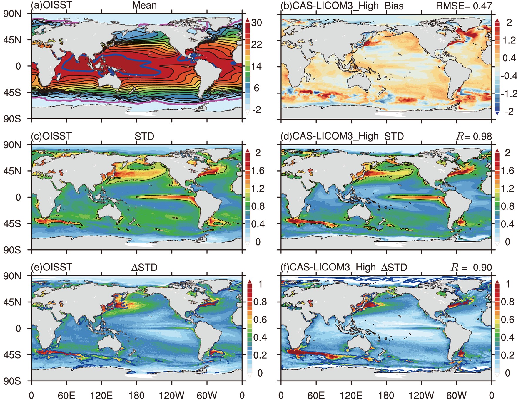 Figure3. Climatological annual mean SST (unit: °C) from (a) OISSTv2 and (b) the biases of CAS-LICOM3_High during 1982–2018 against OISSTv2. The blue and magenta lines in (a) are the 28°C and 0°C isotherms, respectively. (c, d) De-seasonalized STD of daily SST (STD; unit: °C) from (c) OISSTv2 and (d) CAS-LICOM3_High during 1982–2018. (e, f) As in (c, d) but for the ?STD by subtracting the STD of 3° × 3° low-pass filtered monthly SST from the STD of daily SST during 1982–2018. The black contours in (c, d) are the 1°C isotherms. The blue contours in (e, f) are the ratio of 0.5 between ?STD and STD. The RMSE and pattern correlation coefficients (R) between observation and CAS-LICOM3_High are also provided in the figures.
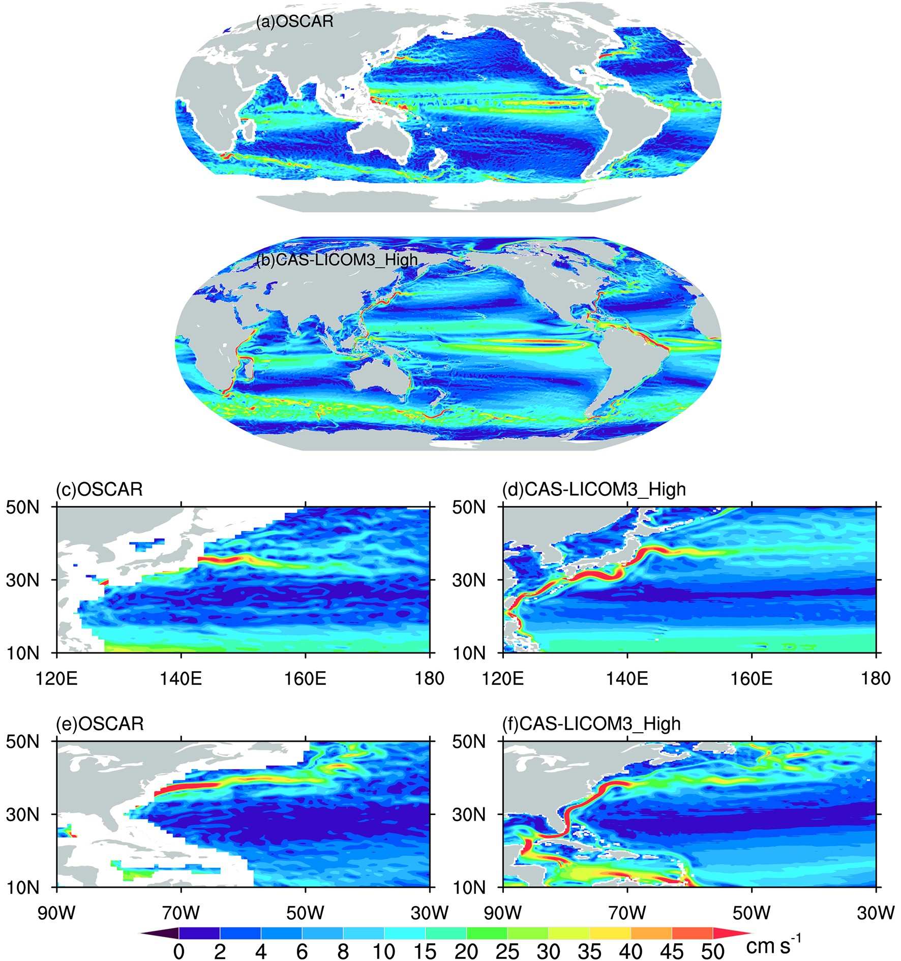 Figure4. Climatological annual mean velocity of ocean surface currents from OSCAR during 1993–2018 for the (a) global, (c) Kuroshio and its extension, and (e) Gulf Stream regions. (b, d, f) As in (a, c, e) but from CAS-LICOM3_High (units: cm s?1).
The de-seasonalized STDs of the daily SST anomaly from OISSTv2 and CAS-LICOM3_High are shown in Figs. 3c and d. The spatial pattern of STDs is simulated well, with a global spatial correlation coefficient of 0.98 between CAS-LICOM3_High and OISSTv2. The large STD values (> 1°C) are located in the equatorial Pacific, western boundary currents and their extensions, the Argentine Basin, and the Southern Ocean between the Indian Ocean and Atlantic Ocean. In the equatorial Pacific, the large STD is mainly due to the interannual variability associated with ENSO, and partly due to the intraseasonal variability related to eddy-induced TIWs. However, there are some underestimations of the simulated STD (Fig. 3d) over the warm SST regions (> 26°C contour lines in Fig. 3a).
Figures 3e and f show the difference between the daily SST STD and 3° × 3° lowpass-filtered monthly SST STD (ΔSTD). The difference indicates the variability due to the highpass signal related to mesoscale activities. As Figs. 3c and d show in the observation and CAS-LICOM3_High, large daily SST STDs are located in the eddy-rich regions, such as the western boundary and ACC. In those places, ΔSTD can reach 1°C (Figs. 3e and f). These large ΔSTD values are attributable to mesoscale eddies, which means the mesoscale signal can contribute to 50% of the total STD of daily SST (Figs. 3e and f). Meanwhile, in the eastern part of the Pacific, mesoscale eddies can contribute to 20% of the STD in the observation and relatively less in CAS-LICOM3_High.
2
3.4. Surface ocean currents
The global large-scale surface current velocity during 1993–2018 for both the Ocean Surface Current Analyses Real-time (OSCAR;For the western boundary currents, the simulated Kuroshio path flows along the shelf break inside the East China Sea between Taiwan Island and Yonaguni-jima Island, which is also proven by observations and other numerical simulations (Johns et al., 2001; Yang et al., 2012). The Gulf Stream in CAS-LICOM3_High can extend to 40°W, but it does not extend as a coherent feature past the New England seamounts, which is also exhibited in the 1/25° simulation from Chassignet and Xu (2017). However, there is a bias about the western boundary currents, as the separation of both the Kuroshio and Gulf Stream shifts northward by about 2° of latitude, compared with OSCAR.
2
3.5. NEUC
The zonal belt structure of the zonal currents are important features for the global ocean, which also cannot be simulated by coarse-resolution models. As discussed in Li et al. (2018), the simulation of the NEUC requires both a high-resolution and long-term simulation, thus meaning the NEUC is a good metric to evaluate high-resolution and long-term simulations. As presented in Fig. 5, the meridional sections of zonal velocity averaged over 135°–140°E, 175°–180°E, and 150°–145°W, from 11-year mean Argo data (Roemmich and Gilson, 2009) and CAS-LICOM3_High, show three branches of NEUCs (Qiu et al., 2013), in all three meridional sections. The Argo zonal velocities are estimated from the density gradients calculated based on the observed temperature and salinity. The upper boundary of the three NEUC jets for CAS-LICOM3_High become deeper with increasing latitude and shallower from west to east, which is exactly the same as in Argo. Although the locations of the NEUC jets are reproduced very well by CAS-LICOM3_High, their strength in CAS-LICOM3_High is weaker than in Argo, which may be related to the non-geostrophic velocity (Li et al., 2018) or the relatively large viscosity in the model. Figure5. (a) The 11-year mean zonal velocity (shading; units: cm s?1) averaged over 135°–140°E (left), 175°–180°E (middle), and 150°–145°W (right) for Argo during 2004–2014. (b) As in (a) but for CAS-LICOM3_High. The zero contours are shown as solid contours.
In summary, CAS-LICOM3_High can reproduce well the long-term trend and interannual–decadal variability of various variables. The refined resolution simulation can not only capture the mesoscale eddies, the western boundary currents, and the zonal jets, but also improve the representation of large-scale circulations. In addition, the mesoscale activities can affect the magnitude of the variabilities, as the mesoscale signal is responsible for up to 50% of the variability of daily SST in eddy-rich regions. The processes related to these variabilities can be further investigated using this dataset and the added value of the high resolution can also be evaluated by comparing with the low-resolution simulation, particularly where the biases have been significantly reduced. In addition, this preliminary evaluation also indicates some systematic biases in the global temperature and salinity, the EKE, and regional current patterns. We will further improve the model in the future.
| Level | T-grid | W-grid |
| 1 | 2.50 | 0.00 |
| 2 | 7.51 | 5.00 |
| 3 | 12.56 | 10.02 |
| 4 | 17.67 | 15.10 |
| 5 | 22.86 | 20.24 |
| 6 | 28.15 | 25.48 |
| 7 | 33.57 | 30.83 |
| 8 | 39.14 | 36.32 |
| 9 | 44.87 | 41.96 |
| 10 | 50.79 | 47.78 |
| 11 | 56.90 | 53.79 |
| 12 | 63.22 | 60.01 |
| 13 | 69.76 | 66.44 |
| 14 | 76.54 | 73.09 |
| 15 | 83.55 | 79.98 |
| 16 | 90.81 | 87.12 |
| 17 | 98.31 | 94.49 |
| 18 | 106.05 | 102.12 |
| 19 | 114.04 | 109.98 |
| 20 | 122.26 | 118.09 |
| 21 | 130.72 | 126.44 |
| 22 | 139.40 | 135.01 |
| 23 | 148.29 | 143.79 |
| 24 | 157.37 | 152.78 |
| 25 | 166.64 | 161.96 |
| 26 | 176.07 | 171.32 |
| 27 | 185.65 | 180.83 |
| 28 | 195.36 | 190.48 |
| 29 | 205.17 | 200.24 |
| 30 | 215.06 | 210.10 |
| 31 | 225.01 | 220.02 |
| 32 | 235.00 | 230.00 |
| 33 | 245.00 | 240.00 |
| 34 | 257.08 | 250.00 |
| 35 | 275.35 | 264.15 |
| 36 | 303.81 | 286.54 |
| 37 | 346.28 | 321.09 |
| 38 | 406.31 | 371.48 |
| 39 | 487.12 | 441.14 |
| 40 | 591.53 | 533.09 |
| 41 | 721.96 | 649.98 |
| 42 | 880.31 | 793.95 |
| 43 | 1067.98 | 966.68 |
| 44 | 1285.80 | 1169.28 |
| 45 | 1534.07 | 1402.32 |
| 46 | 1812.49 | 1665.81 |
| 47 | 2120.22 | 1959.17 |
| 48 | 2455.88 | 2281.28 |
| 49 | 2817.55 | 2630.48 |
| 50 | 3202.83 | 3004.62 |
| 51 | 3608.89 | 3401.05 |
| 52 | 4032.51 | 3816.78 |
| 53 | 4470.13 | 4248.28 |
| 54 | 4917.95 | 4691.98 |
| 55 | 5371.96 | 5143.91 |
| 56 | 5600.00 |
TableB. Depth of model levels for T- and W-grid.
There are 23 variables and 4 parameters provided in this dataset, including daily and monthly SSS, SST and SSH. The monthly three-dimensional ocean temperature, salinity and ocean velocities are also included. The monthly global mean temperature, salinity and AMOC are also uploaded in the dataset. Information on the data grid, such as area, mask, cell thickness and volume for every ocean grid, is also provided. The detail of each variable can be found in Appendix C, Table C.
| Name | Description | Horizontal resolution | Vertical resolution | Frequency |
| mlotst | Ocean mixed-layer thickness defined by sigma-T | 25 km | 1 layer | Monthly |
| msftmz | Ocean meridional overturning mass streamfunction | 50 km | 55 layers | Monthly |
| so | Seawater salinity | 25 km | 55 layers | Monthly |
| soga | Global mean seawater salinity | ? | ? | Monthly |
| sos | Sea surface salinity | 25 km | 1 layer | Monthly |
| sosga | Global average sea surface salinity | ? | ? | Monthly |
| thetao | Seawater potential temperature | 25 km | 55 layers | Monthly |
| thetaoga | Global average seawater potential temperature | ? | ? | Monthly |
| tos | Sea surface temperature | 25 km | 1 layer | Monthly |
| tosga | Global average sea surface temperature | ? | ? | Monthly |
| uo | Seawater X-velocity | 25 km | 55 layers | Monthly |
| vo | Seawater Y-velocity | 25 km | 55 layers | Monthly |
| wo | Seawater vertical velocity | 25 km | 55 layers | Monthly |
| zos | Sea surface height above geoid | 25 km | 1 layer | Monthly |
| tob | Seawater potential temperature at sea floor | 25 km | 1 layer | Monthly |
| sob | Seawater salinity at sea floor | 25 km | 1 layer | Monthly |
| amoc_rapid | Mean max AMOC at 26°N | ? | ? | Monthly |
| smoc | Mean at 34°S for maximum streamfunction for AMOC | ? | ? | Monthly |
| mfo_drake | Monthly Drake Passage transport | ? | ? | Monthly |
| mfo_indo | Monthly Indonesian Throughflow transport | ? | ? | Monthly |
| sos | Sea surface salinity | 25 km | 1 layer | Daily |
| tos | Sea surface temperature | 25 km | 1 layer | Daily |
| zos | Sea surface height above geoid | 25 km | 1 layer | Daily |
| areacello | Grid-cell area for ocean variables | 25 km | 1 layer | Fixed |
| deptho | Sea floor depth below geoid | 25 km | ? | Fixed |
| thkcello | Ocean model cell thickness | 25 km | 55 layers | Fixed |
| volcello | Ocean grid-cell volume | 25 km | 55 layers | Fixed |
TableC. Description of dataset variables.
This appendix describes the experiment design of CAS-LICOM3_Low and compares it with CAS-LICOM3_High.
CAS-LICOM3_Low shares most settings with CAS-LICOM3_High, but there are some differences. First, CAS-LICOM3_Low uses the PHC3.0 temperature and salinity as the initial state. In CAS-LICOM3_Low, the Laplacian scheme was used, which is different from the biharmonic scheme in CAS-LICOM3_High. The biharmonic scheme has the so-called “scale selected” feature. It is more effective to damp the checkerboard noise than the Laplacian scheme. Therefore, the resolved scales are less damped. This is good for the simulation of the mesoscale eddies.
The coupled CICE4 in CAS-LICOM3_Low contains both dynamic and thermodynamic sea-ice processes, while only the thermodynamic process of CICE4 is coupled in CAS-LICOM3_High. The lack of dynamic sea ice can lead to bias in the Arctic, especially for sea-ice volume. A detailed description of the low-resolution dataset can be found in Lin et al. (2020). Table A compares the parameters from CAS-LICOM3_Low and CAS-LICOM3_High.
| CAS-LICOM3_High | CAS-LICOM3_Low | |
| Horizontal grid spacing | 1/10° (11 km in longitude, about 11 km at the equator, and 8 km at midlatitudes) | 1° (110 km in longitude, about 110 km at the equator, and 80 km at midlatitudes) |
| Explicit horizontal viscosity | Biharmonic A4 = ?2.8 × 10¹⁰ m4 s?1 | Laplacian A2 = 5400 m2 s?1 |
| Explicit vertical viscosity | Background viscosity of 2 × 10?6 m2 s?1 in Canuto et al. (2001, 2002) with upper limit of 2 × 10?2 m2 s?1 | Background viscosity of 2 × 10?6 m2 s?1 in Canuto et al. (2001, 2002) with upper limit of 2 × 10?2 m2 s?1 |
| Explicit Horizontal diffusivity | Biharmonic A4 = ?2.8 × 10¹⁰ m2 s?1 | Laplacian A2 = 5400 m2 s?1 |
| Explicit vertical diffusivity | Background viscosity of 2 × 10?6 m2 s?1 in Canuto et al. (2001, 2002) with upper limit of 2 × 10?2 m2 s?1 | Background viscosity of 2 × 10?6 m2 s?1 in Canuto et al. (2001, 2002) with upper limit of 2 × 10?2 m2 s?1 |
| Isopycnal scheme, e.g., GM | No GM and Redi, Biharmonic A4 = ?2.8 × 10¹⁰ m4 s?1 | Both Redi and GM with the same coefficient computed by Ferreira et al. (2005) |
| Mixed layer scheme | Canuto et al. (2001, 2002) | Canuto et al. (2001, 2002) |
| Advection scheme | Leapfrog for momentum; two step preserved shape advection scheme for tracer (Yu, 1994) | Leapfrog for momentum; two step preserved shape advection scheme for tracer (Yu, 1994) |
| Time stepping scheme | Split-explicit Leapfrog with Asselin filter (0.2 for barotropic; 0.43 for baroclinic; 0.43 for tracer) | Split-explicit Leapfrog with Asselin filter (0.2 for barotropic; 0.43 for baroclinic; 0.43 for tracer) |
| Bottom drag | Cb = 2.6 × 10?3 | Cb = 2.6 × 10?3 |
| Surface wind-stress | Absolute wind stress | Absolute wind stress |
| Vertical coordinates | 55 $ \eta $ levels | 30 $ \eta $ levels |
| SSS restoring | 50 m (4 yr)?1; 50 m (30 d)?1 for sea-ice region | 50 m (4 yr)?1; 50 m (30 d)?1 for sea-ice region |
TableA. Comparison between CAS-LICOM3_High and CAS-LICOM3_Low.
Acknowledgements. This study was supported by National Key R&D Program for Developing Basic Sciences (2018YFA0605703, 2016YFC1401401, 2016YFC1401601), the Strategic Priority Research Program of Chinese Academy of Sciences (Grant No. XDB42010404, XDC01000000), and the National Natural Science Foundation of China (Grants 41976026, 41776030 and 41931183, 41931182, 41576026). The authors acknowledge the technical support from the National Key Scientific and Technological Infrastructure project “Earth System Science Numerical Simulator Facility” (EarthLab).
Open Access This article is distributed under the terms of the Creative Commons Attribution 4.0 International License (
