HTML
--> --> -->Different modes of sea surface temperature (SST) can explain most of the inter-annual and inter-decadal variations of rainfall in China (Yang and Lau, 2004). Two modes of SST that reflect strong climatic teleconnections with the EASM rainfall are El Ni?o and the Pacific Decadal Oscillation (PDO) (Ma, 2007). An El Ni?o event is characterized by anomalous warming in the central and eastern equatorial Pacific Ocean and occurs, on average, every two to seven years. By contrast, the PDO (Mantua et al., 1997; Qian and Zhou, 2014) is marked by an inter-decadal cycle, and is mainly present in the North Pacific (poleward of 20°N). During the warm phase of the PDO, SST tends to be anomalously cool in the central North Pacific, coincident with anomalously warm SST in the eastern North Pacific, whereas the spatial pattern of SST is reversed during the cool phase of the PDO.
Because the inter-annual variability in the atmospheric concentrations of CO2 induced by El Ni?o is mainly attributed to tropical terrestrial ecosystems (Yang and Wang, 2000; Cox et al., 2013; Wang et al., 2013; Liu et al., 2017), previous studies have primarily focused on how terrestrial carbon fluxes in the tropics responding to changes in the Earth’s climate (especially changes in temperature and rainfall) caused by El Ni?o (Gu and Adler, 2011; Bastos et al., 2013; Wang et al., 2016; Fang et al., 2017). The most common way to investigate the decadal variability in the terrestrial carbon budget caused by the PDO is to use the long-term teleconnection between the PDO indices and specific carbon cycle variables (Wharton and Falk, 2016; Zhang et al., 2018). However, this method is unable to reflect the impact of the variability of local chaotic weather events (Ito, 2011), especially when the responses of terrestrial carbon cycle to different El Ni?o events are contrasting (Liu et al., 2017; Wang et al., 2018). Hence, the mixed effects of El Ni?o and the PDO on the carbon cycle in the extratropical monsoon regions of China are still poorly understood.
Even though the spatiotemporal patterns of rainfall anomalies over East Asia associated with individual El Ni?o episodes are variable (Wang et al., 2017), Feng et al. (2014) still found relatively stable relationships between the EASM rainfall and El Ni?o under different phases of the PDO. When the PDO is in a cool phase, with a high-pressure area in the subtropical western Pacific clearly experiencing two northward shifts, positive rainfall anomalies move from southern to northern China. By contrast, when the PDO is in a warm phase, a greater amount of rainfall is observed in central China, whereas less rainfall is observed in southern and northern China. How GPP responds to these specific rainfall patterns is still unclear.
The purpose of this study was to determine the relationship between the GPP and the changes in rainfall associated with El Ni?o under different phases of the PDO in eastern China. In particular, we attempted to identify the regions driving this relationship and to demonstrate the response of GPP to El Ni?o and the PDO. The results may have implications for how terrestrial carbon dynamics responding to variabilities in the Earth’s climate.
2.1. MsTMIP GPP and CRU–NCEP Datasets
The rainfall patterns described in the fourth paragraph of the Introduction were revealed and explained by data spanning from 1957 to 2010. Given the data consistency, this study also focused on the same period and selected the same El Ni?o years (see Table 1) as Feng et al. (2014). Compared with other approaches, the Terrestrial Biosphere Model (TMB) is a preferred method to estimate carbon fluxes over such a long period because of the availability of climate forcing data and process-based simulation. The monthly GPP products of 15 TMBs in the Multi-scale synthesis and Terrestrial Model Intercomparison Project (MsTMIP) (Huntzinger et al., 2013; Wei et al., 2014) were applied here. The MsTMIP version 1.0 dataset includes four global (0.5° × 0.5° resolution) sensitivity simulations (SG1, SG2, SG3 and BG1) which can systematically assess the impacts of different forcing factors. The model-driven data in MsTMIP version 1.0 are climate variables (Climate), land use/land cover changes (LUCC), the atmospheric CO2 concentration (CO2) and nitrogen deposition (N). The time-varying drivers in the four global sensitivity simulations are Climate (SG1), Climate + LUCC (SG2), Climate + LUCC + CO2 (SG3), and Climate + LUCC + CO2 + N (BG1). BG1 only includes a limited number of models as a result of the lack of a nitrogen cycle in other MsTMIP members. SG3 and BG1 are presumed to be closer to reality than SG1 and SG2 and were therefore used in this study. The CLASS-CTEM-N model was excluded because its GPP estimates for China are much lower than is reasonable (Shao et al., 2016).| PDO phase | El Ni?o years and intensities | |||||||
| Warm | Major | Minor | Super | Moderate | Moderate | Major | Super | Moderate |
| 1957 | 1976 | 1982 | 1986 | 1987 | 1991 | 1997 | 2002 | |
| Cool | Minor | Major | Minor | Major | Moderate | Moderate | Minor | Major |
| 1963 | 1965 | 1968 | 1972 | 1994 | 2004 | 2006 | 2009 | |
| Note: The intensities of El Ni?o were categorized as defined in Wang et al. (2017). | ||||||||
Table1. Characteristics of the 16 El Ni?o years in this study.
The available climatology datasets from the Climate Research Unit (CRU) (Harris et al., 2014) and the National Centers for Environmental Prediction (NCEP)/National Center for Atmospheric Research (NCAR) (Kalnay et al., 1996) cannot fully meet the spatial and temporal requirements of MsTMIP. Therefore, a new dataset named CRU-NCEP was produced by combining the strengths of the datasets from the CRU and NCEP/NCAR as driver data for MsTMIP. The CRU–NCEP dataset not only maintains a good match to the observed rainfall in China (Zhao and Fu, 2006), but also corrects the known biases in temperature and downward shortwave radiation in the NCEP/NCAR reanalysis products (Wei et al., 2014). Therefore, the globally gridded (0.5° × 0.5°) and monthly CRU-NCEP dataset was chosen to determine the relationships between GPP and the particular meteorological factors (rainfall, temperature, and downward shortwave radiation).
2
2.2. Bayesian Model Averaging
Eight typical ChinaFLUX sites (see Appendix A.1) were selected to validate modeled GPP. After comparing with the observed GPP from ChinaFLUX, it was found that there were large uncertainties in the MsTMIP GPP (see Appendix A.2). Selecting only one model may lead to statistical biases and an underestimation of the uncertainties (Neuman, 2003; Raftery et al., 2005). Bayesian model averaging (BMA) (Hoeting et al., 1999) can effectively solve this problem. After comprehensively considering the conditional distribution of each ensemble member, BMA takes the maximum of the probability density function (PDF) as an individual model’s weighted coefficient following a training process. Thus, the final weighted average results reflect each model’s optimum contribution to the quantities of interest (Wasserman, 2000). We used the MATLAB toolbox provided by Vrugt (2016) to implement BMA. The core mathematical expressions are as follows. If


The optimum of the likelihood function is:
After implementation of training with data


The plant function types (PFTs) were simply merged into three classes (trees, grasses, and crops) when the BMA was trained during 2003–08 (see Appendix A.3). Before the weighted coefficients for different models were used at the regional scale, they needed to be further modified depending on the proportion of land cover types in each grid cell. If the BMA weighted coefficients trained in the ChinaFLUX sites for


where


2
2.3. Data Preprocessing
To highlight the impact of the EASM on GPP, May and September were defined as the start and end months of the growing season corresponding to the onset and withdrawal months of the EASM. When analyzing the response characteristics of GPP to El Ni?o over China and the corresponding mechanism, GPP and the meteorological data were not only limited to the growing season in each year, but also were detrended to minimize the possible influence of long-term trends. Trends were calculated by simple linear regression.3.1. Validation of the BMA GPP at the ChinaFLUX Sites
The MsTMIP and BMA GPP data in the grid cells containing ChinaFLUX sites from 2009 to 2010 were chosen to evaluate the rationality of using BMA. The efficiency criteria used in this section are Ef indices (see Appendix A.4). The Ef indices for different models are listed in Table 2. BMA performed better than the MsTMIP models in the qualified grid cells corresponding to Changbaishan, Qianyanzhou, Yucheng, and Inner Mongolia, thereby proving its strength for the typical PFTs at these sites. Even though the Ef indices calculated in the grid cells for Dinghushan and Haibei were not statistically significant, the relatively small absolute values still indicated that the magnitude of the BMA GPP was acceptable, especially in the subtropical region where Dinghushan is located. The evergreen broad leaf trees in Xishuangbanna and the grasses in Dangxiong are rainforests and alpine meadows, respectively, and the negative Ef indexes suggested that the manner in which BMA was used in this study was unable to reduce the uncertainties from these two specific PFTs.| Model Name | Site | |||||||
| Changbaishan | Qianyanzhou | Dinghushan | Xishuangbanna | Yucheng | Inner Mongolia | Haibei | Dangxiong | |
| BIOME–BGC | 0.84 | –0.20 | –3.20 | –1.68 | –0.54 | 0.29 | –0.56 | 0.82 |
| CLM4 | 0.82 | –8.53 | –62.37 | –1.34 | –0.15 | 0.46 | –0.23 | –7.82 |
| CLM4VIC | 0.91 | –4.49 | –61.78 | –3.05 | –0.37 | –0.39 | –0.83 | –7.74 |
| DLEM | 0.42 | 0.24 | –0.87 | 0.68 | 0.06 | –0.67 | –0.53 | 0.16 |
| GTEC | 0.96 | –1.54 | –3.27 | –8.74 | –0.07 | –2.03 | 0.60 | –5.68 |
| ISAM | 0.78 | 0.76 | –2.07 | –0.65 | –0.52 | 0.34 | –0.53 | –1.31 |
| LPJ–wsl | 0.94 | –0.32 | –5.07 | –2.22 | –0.08 | 0.06 | –0.47 | –48.65 |
| ORCHIDEE–LSCE | 0.88 | 0.17 | –15.43 | –5.06 | 0.16 | 0.23 | 0.51 | –44.53 |
| SiB3 | 0.91 | 0.52 | –14.52 | –2.35 | 0.50 | –0.16 | –0.68 | 0.57 |
| SiBCASA | 0.89 | –0.27 | –7.27 | –6.30 | 0.40 | 0.35 | –0.31 | 0.27 |
| TEM6 | 0.86 | –1.17 | –2.17 | –1.05 | –0.89 | 0.22 | –0.32 | 0.39 |
| TRIPLEX–GHG | 0.56 | –1.25 | –27.17 | –4.54 | 0.09 | 0.36 | 0.01 | –10.68 |
| VEGAS2.1 | 0.49 | 0.56 | –9.17 | 0.47 | –0.16 | –0.06 | 0.19 | –1.51 |
| VISIT | 0.89 | –2.51 | –54.13 | –1.11 | –0.98 | –0.20 | –0.93 | –0.26 |
| BMA | 0.95 | 0.81 | –4.62 | –1.11 | 0.27 | 0.31 | –0.01 | –0.59 |
Table2. Nash–Sutcliffe efficiency index values for GPP simulated by 14 terrestrial biosphere models and Bayesian model averaging at eight ChinaFLUX sites.
2
3.2. The Response of GPP to El Ni?o in Different Phases of the PDO
Figure 1 shows the average spatial anomalies of the BMA GPP and the CRU–NCEP rainfall for the selected El Ni?o years with different phases of the PDO. The GPP and rainfall with large anomalies were mainly distributed in northern China (32°–38°N, 111°–122°E) and the Yangtze River valley (28°–32°N, 111°–122°E). The similar spatial distribution of the GPP and the rainfall anomalies shown in Fig. 1 indicate that rainfall is the connection between the El Ni?o and GPP in eastern China (28°–38°N, 111°–122°E). Figure1. Spatial anomalies of BMA GPP during the growing season (May–September) averaged from El Ni?o years under (a) the cool phase of the PDO and (b) the warm phase of the PDO in China. (c) and (d) are the same as (a) and (b) respectively, but for rainfall. The anomalies are relative to the mean of the time period 1957–2010. The dashed lines denote negative anomalies and the colored areas denote positive anomalies. The target zones (28°–32°N, 111°–122°E; 32°–38°N, 111°–122°E) are shown by the rectangles. GPP and rainfall were detrended in advance.
The spatial anomalies of the GPP averaged from multiple El Ni?o years (Fig. 1a, Fig. 1b) leads to the following hypotheses: (1) the zone in which GPP was significantly affected by El Ni?o was in eastern China (28°–38°N, 111°–122°E); (2) when the El Ni?o years were in the cool phase of the PDO, GPP was higher in northern China (32°–38°N, 111°–122°E) and lower in the Yangtze River valley (28°–32°N, 111°–122°E); and (3) when the El Ni?o years were in the warm phase of the PDO, the spatial anomaly patterns of the GPP in these two regions were reversed.
To check whether these hypotheses are valid, the response of GPP to each El Ni?o year was analyzed. Figure 2 shows the spatial anomalies of GPP in eight typical El Ni?o years under the cool phase of the PDO. Except for 1968 and 1994, the graphs for other years in Fig. 2 all support these hypotheses and the most positive anomalies in northern China (32°–38°N, 111°–122°E) were statistically significant.
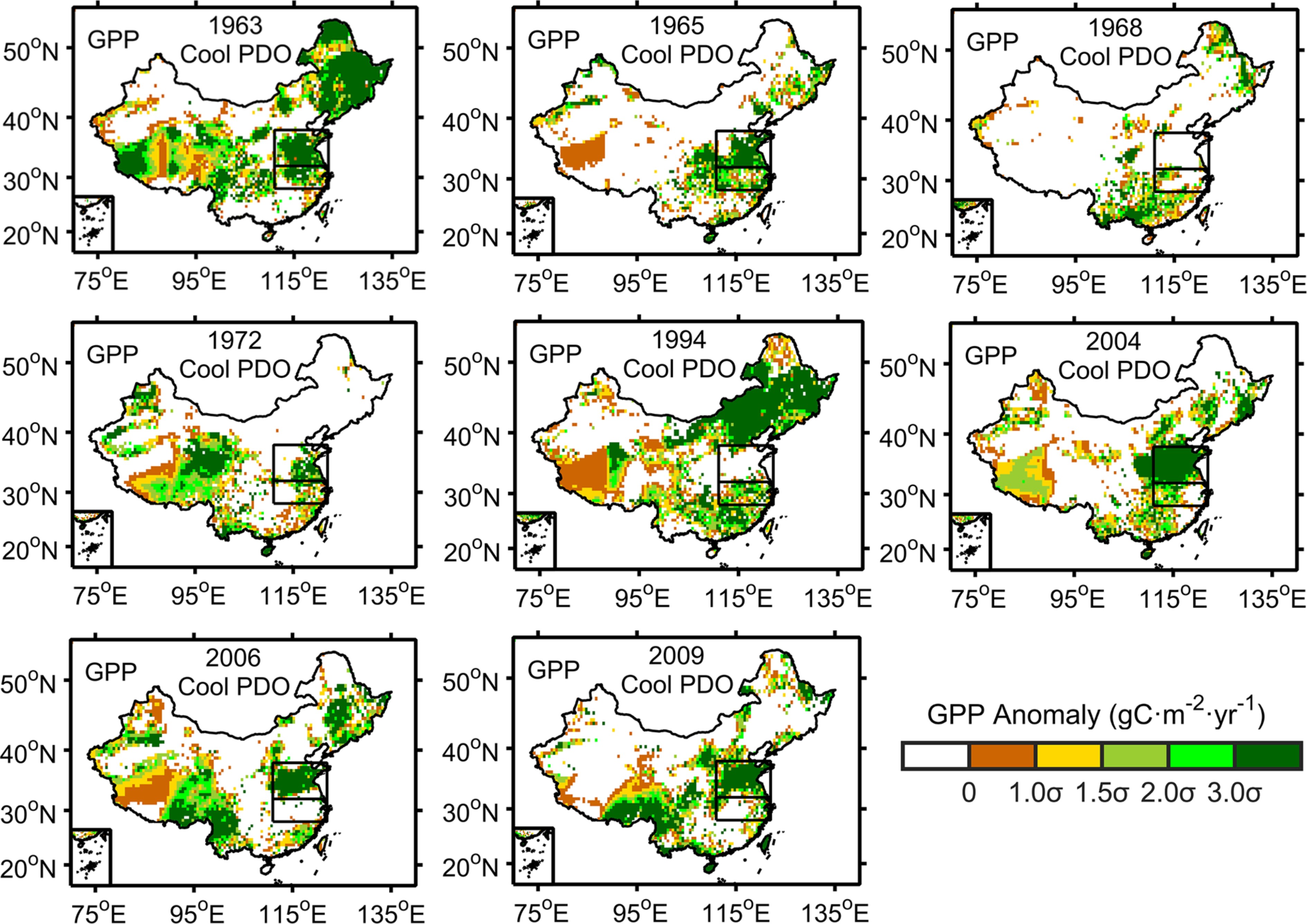 Figure2. Spatial anomalies of BMA GPP during the growing season (May–September) for eight selected El Ni?o years under the cool phase of the PDO in China. The anomalies are relative to the mean of the time period 1957–2010. The blank areas denote negative anomalies and the colored areas denote positive anomalies. The target zones (28°–32°N, 111°–122°E; 32°–38°N, 111°–122°E) are shown by the rectangles. σ is the standard deviation of the BMA GPP anomalies, where ≥1.5σ means that the positive anomalies are significant. GPP was detrended in advance.
Figure 3 shows the spatial anomalies of GPP in eight typical El Ni?o years under the warm phase of the PDO. Excluding 1957 and 1976, the positive anomalies of GPP for the remaining El Ni?o years were mainly distributed in the Yangtze River valley (28°–32°N, 111°–122°E), which further verified the hypotheses from the averaged El Ni?o years. Less significant positive GPP anomalies were found in the Yangtze River valley. This difference suggests that plants in northern China are more sensitive to El Ni?o than those in the Yangtze River valley.
 Figure3. Spatial anomalies of BMA GPP during the growing season (May–September) for eight selected El Ni?o years under the warm phase of the PDO in China. The anomalies are relative to the mean of the time period 1957–2010. The blank areas denote negative anomalies and the colored areas denote positive anomalies. The target zones (28°–32°N, 111°–122°E; 32°–38°N, 111°–122°E) are shown by the rectangles. σ is the standard deviation of the BMA GPP anomalies, where ≥1.5σ means that the positive anomalies are significant. GPP were detrended in advance.
The evolution of the zonal-time anomaly (May–September) of rainfall and GPP averaged from 111° to 122°E for typical El Ni?o years in the cool and warm phases of the PDO are shown in Fig. 4 and Fig. 5. Even when there are some deflections, it is still clear that the large anomalies in the rainfall and GPP are synchronized both spatially and temporally. This confirms that the close relationship between GPP and El Ni?o in eastern China is related to the north–south movement of the rain belt.
 Figure4. Latitude–time cross-sections of the (a) rainfall (mm yr?1) and (b) BMA GPP (gC m?2 yr?1) anomalies during the growing season (May–September) for El Ni?o years under the cool phase of the PDO in eastern China (28°–38°N, 111°–122°E). The dashed lines denote negative anomalies and the colored areas denote positive anomalies. GPP and rainfall were detrended in advance.
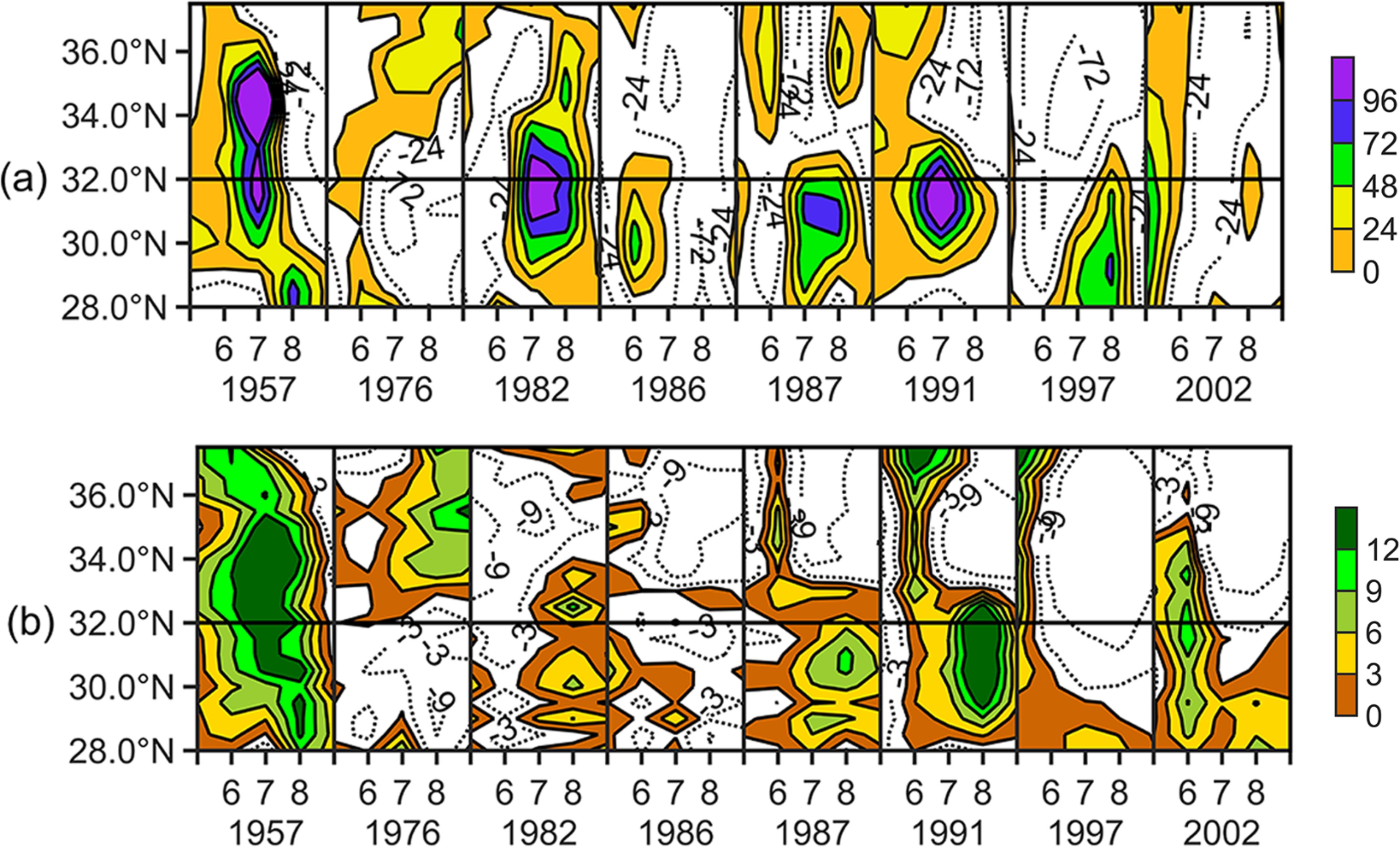 Figure5. Latitude–time cross-sections of the (a) rainfall (mm yr?1) and (b) BMA GPP (gC m?2 yr?1) anomalies during the growing season (May–September) for El Ni?o years under the warm phase of the PDO in eastern China (28°–38°N, 111°–122°E). The dashed lines denote negative anomalies and the colored areas denote positive anomalies. GPP and rainfall were detrended in advance.
2
3.3. The Solid Relationship between GPP and Rainfall in Eastern China
The inter-annual relationships between meteorological factors and vegetation activity can be changed in different decades (Piao et al., 2014). The EASM weakened from the late 1970s but has gradually recovered since the early 1990s (Liu et al., 2012). Two abrupt climate change points are recognized in 1978 and 1992 (Ding et al., 2008). To determine whether the relationships between GPP and the particular meteorological factors (rainfall, temperature, and the downward shortwave radiation) are consistent under different EASM intensities, they were compared in different time periods (1957–78, 1979–92, and 1993–2010).To confirm the role of key meteorological factors for GPP, partial correlations between GPP and rainfall, downward shortwave radiation, and temperature in China are given in Fig. 6. This analysis shows that rainfall dominated the inter-annual changes of the GPP in eastern China from 1957 to 2010. By contrast, the roles of temperature and downward shortwave radiation in the same region were rather limited, although the effect of temperature was clearer in the time period 1957–78. The bar diagrams in Fig. 7 show the proportions of partial correlations between GPP and the particular meteorological factors in northern China and the Yangtze River valley, respectively. The highest proportions of positive partial correlations are between GPP and rainfall in all periods in Fig. 7, which clearly shows the importance of rainfall. The results in this section further enhance the credibility of the response characteristics of GPP to El Ni?o in eastern China being mostly due to its close relationship with rainfall.
 Figure6. Spatial patterns of partial correlations between the growing season (May–September) BMA GPP and (a) rainfall (RAIN), (b) downward shortwave radiation (DWSR), and (c) temperature (TEMP) in China in 1957–78. (d), (e), and (f) are the same as (a), (b), and (c), respectively, but in 1979–92. (g), (h), and (i) are also the same as (a), (b), and (c), respectively, but in 1993–2010. Gray regions indicate insignificant partial correlations (P > 0.05). The target zones (28°–32°N, 111°–122°E; 32°–38°N, 111°–122°E) are shown by rectangles. The GPP and meteorological factors were detrended in advance.
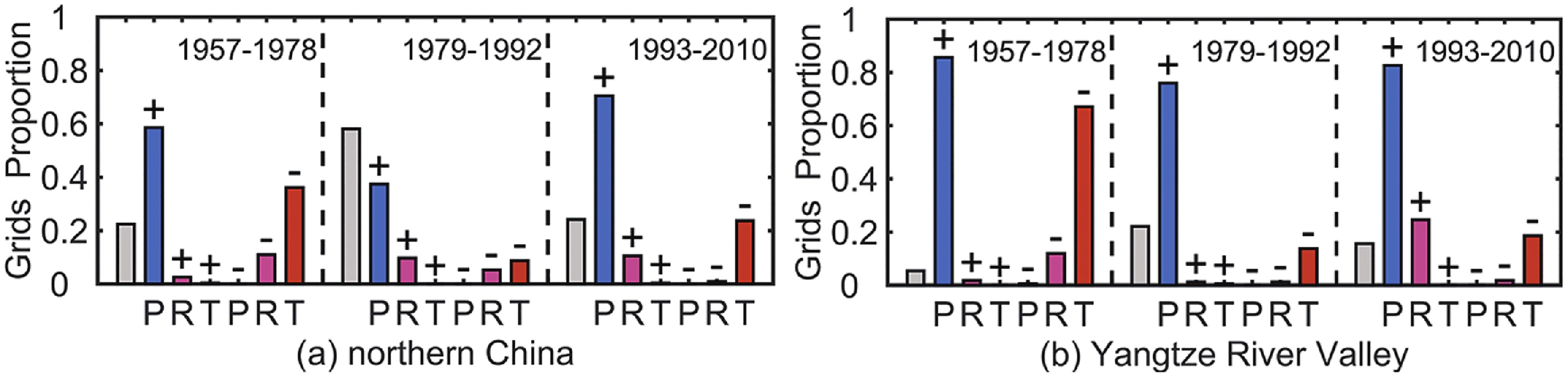 Figure7. Proportions of positive (+) and negative (–) partial correlations between the growing season (May–September) BMA GPP and rainfall (P), temperature (T), and downward shortwave radiation (R) in (a) northern China (32°–38°N, 111°–122°E) and (b) the Yangtze River valley (28°–32°N, 111°–122°E) in strong and weak East Asian Summer Monsoon periods (1957–78, 1979–92, and 1993–2010). Gray bars indicate the proportions of insignificant partial correlations. All data were detrended in advance.
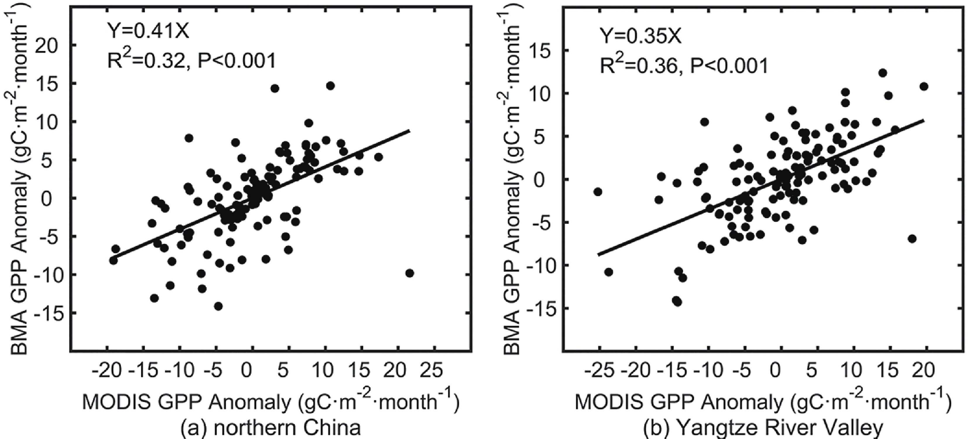 Figure8. Anomaly scatterplots of the monthly MODIS GPP against the monthly BMA GPP averaged in (a) northern China (32°–38°N, 111°–122°E) and (b) the Yangtze River valley (28°–32°N, 111°–122°E) in the time period 2000–10. All of the GPP data were detrended in advance.
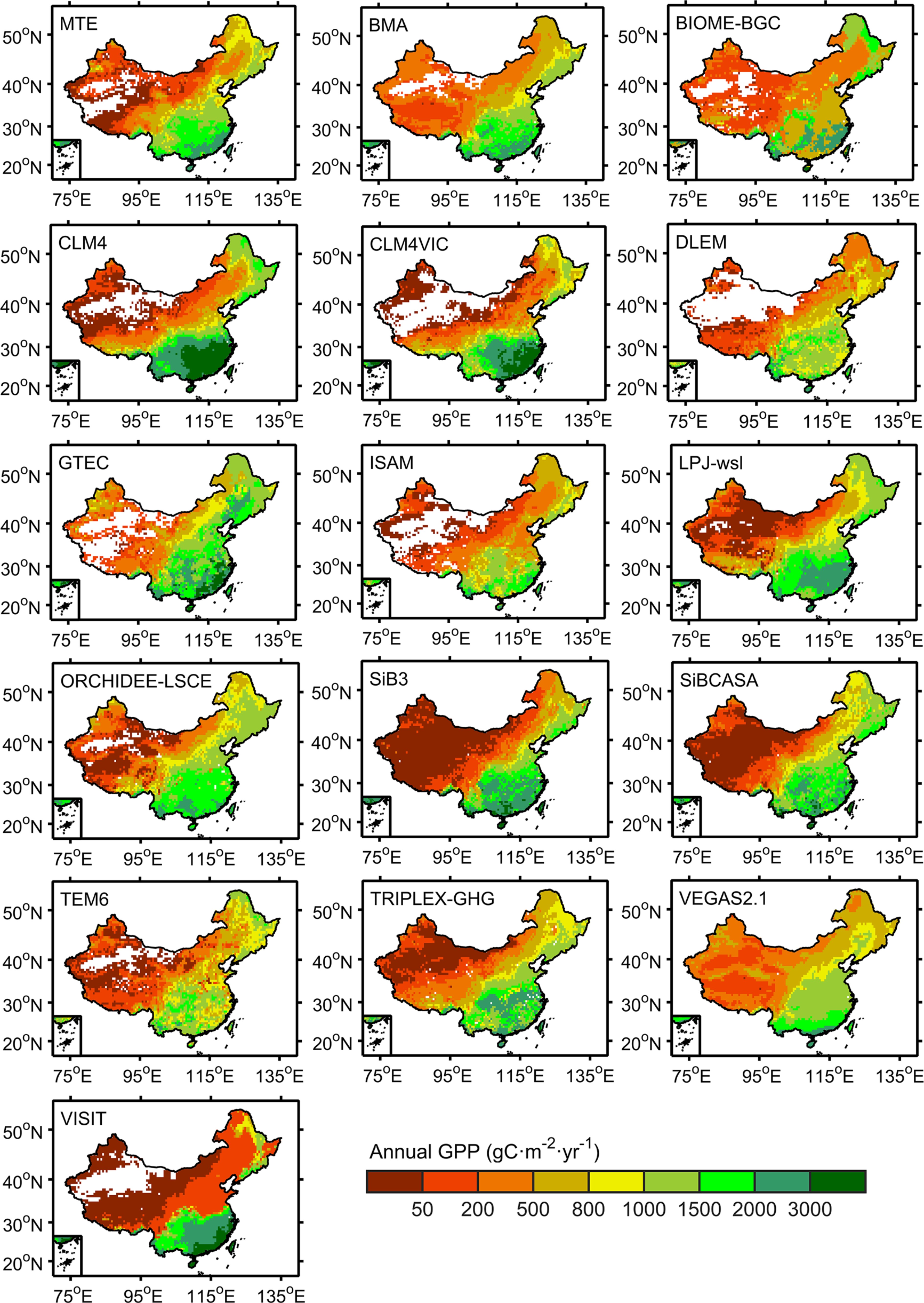 Figure9. Spatial patterns of the annual GPP in China averaged from MTE, BMA, and the various MsTMIP model contributors during 1982?2010.
The general consensus is that GPP in the tropics is usually reduced due to the warm and dry conditions caused by El Ni?o (Cavaleri et al., 2017; Yang et al., 2018; Qian et al., 2019; Yan et al., 2019). By contrast, the current study was carried out in the temperate zone (28°–38°N, 111°–122°E) of China. We found that GPP was not simply increased or decreased, but showed opposite north–south anomalies (divided by 32°N) when El Ni?o occurred under different phases of the PDO. However, the spatial anomalies of the BMA GPP in eastern China for 1957, 1968, 1976, and 1994 did not follow the general pattern seen in most selected El Ni?o years. This inconsistency suggests that using a combination of El Ni?o and the phase of the PDO to predict GPP is not completely reliable. The misplacement of the BMA GPP anomalies in eastern China for 1968 (minor El Ni?o) compared with 2006 (minor El Ni?o), 1994 (moderate El Ni?o) compared with 2004 (moderate El Ni?o), and 1957 (major El Ni?o) compared with 1991 (major El Ni?o) also indicates that a classification of the El Ni?o event as “strong” or “weak” is not sufficient to judge the inter-annual variations in the GPP. The diversities in how GPP responds to different El Ni?o episodes further complement and deepen our understanding of the nonlinear climatic effects of sea surface temperature on local plants.
The inter-annual variabilities of the GPP derived from eddy covariance network observations are controlled by rainfall in temperate regions (Jung et al., 2011), which is consistent with the results in this study. The different responses of GPP to El Ni?o in tropical and temperate regions are seen not only for the enzyme-driven land surface models in this paper, but are also reported for the model driven by remote sensing data (Zhang et al., 2019b). Specific terrestrial biosphere models (e.g., DLEM, LPJ, VEGAS, VISIT, CLM, ISAM, and ORCHIDEE) with a proven ability to reproduce the deviations in carbon flux caused by El Ni?o (Wang et al., 2016; Chang et al., 2017; Bastos et al., 2018) also took part in MsTMIP and contributed to the BMA GPP. Therefore, our conclusions based on the BMA GPP are credible.
The GPP in eastern China is difficult to describe quantitatively as a result of the uncertainties in the modeled GPP and the variety of climatic effects from different El Ni?o events (Schwalm et al., 2011), therefore the responses of GPP to El Ni?o are only qualitatively shown here. This study only focused on the inter-annual relationships between different climate variables (rainfall, temperature, and downward shortwave radiation) and GPP, so the roles of specific climate changes (e.g., an increase/decrease in the intensity or frequency of rainfall) were neglected. Given the complexities of the Earth’s climate system, the physical mechanisms in dry episodes associated with El Ni?o and the resulting state of the vegetation in eastern China still require further research. TBMs simulated the physiological processes of crops more poorly than other PFTs that were less affected by human activities (see Appendix A.2). A benefit from the advantages of the BMA method is that this defect in eastern China where crops occupy a large proportion of the area can be minimized by weighting different models according to their performance. Additionally, the intensity of agricultural management (especially irrigation) is difficult to evaluate at a regional level, so its impacts on the conclusions found in this study also need further investigation.
In contrast to the tropics, where it is generally believed that local plant physiology can be significantly affected by El Ni?o, this paper focused on the neglected eastern monsoon region of China. The spatial anomalies of BMA GPP averaged from the multiple El Ni?o years in different phases of PDO produced the following hypothesis: El Ni?o during the cool phase of the PDO led to greater GPP in northern China (32°–38°N, 111°–122°E) and less GPP in the Yangtze River valley (28°–32°N, 111°–122°E); but El Ni?o during the warm phase of PDO reversed the GPP anomalies in these two regions. Even though there were some discrepancies, most individual El Ni?o years supported the hypothesis mentioned above, and therefore the conclusions have high applicability. It should also be noted that the effects of El Ni?o are more significant in northern China than in the Yangtze River valley.
The synchronized spatiotemporal distribution in selected El Ni?o years and high partial correlation both in strong and weak periods of the EASM all demonstrated that rainfall linked El Ni?o and GPP in eastern China. Although EASM systems are complex (Ding and Chan, 2005) and the movements of the EASM rain belt are difficult to forecast (Gao et al., 2011, 2014; Fan et al., 2012), this study showed that we can still predict how GPP will change in eastern China (28°–38°N, 111°–122°E) when El Ni?o occurs if we can identify the phase of the PDO. The results of this study also provide a reference for future research on the impact of El Ni?o on the carbon cycle of terrestrial ecosystems in China.
Acknowledgments. This study was jointly supported by the National Key Research and Development Program of China (Grant Nos. 2016YFA0602501 and 2018YFA0606004) and the Strategic Priority Research Program of the Chinese Academy of Sciences (Grant Nos. XDA20040301 and XDA20020201).
APPENDIX A.1 Observed GPP from ChinaFLUX
The monthly observed GPP data from eight typical flux measurement sites in the ChinaFLUX network (Yu et al., 2006) were used to validate the modeled GPP. The selected eddy covariance tower sites cover all the main ecosystem types in China and have been successfully applied to validate the performance of different models (Li et al., 2013; Wang et al., 2015; Zhang et al., 2016). Detailed information about these sites is given in Table A1.| Site | Latitude (°N) | Longitude (°E) | Time period | Biome type | Biome classification |
| Changbaishan | 42.40 | 128.10 | 2003–10 | DMT | Trees |
| Qianyanzhou | 26.74 | 115.06 | 2003–10 | ENT | Trees |
| Dinghushan | 23.17 | 112.53 | 2003–10 | EBT | Trees |
| Xishuangbanna | 21.93 | 101.27 | 2003–10 | EBT | Trees |
| Yucheng | 36.83 | 116.57 | 2003–10 | CRO | Crops |
| Inner Mongolia | 43.33 | 116.40 | 2004–10 | GRA | Grasses |
| Haibei | 37.62 | 101.32 | 2003–10 | SHB | Grasses |
| Dangxiong | 30.50 | 91.07 | 2004–10 | GRA | Grasses |
| DMT: Deciduous Mixed Leaf Trees; ENT: Evergreen Needle Leaf Trees; EBT: Evergreen Broad Leaf Trees; CRO: Crops; GRA: Grasses; SHB: Shrubs. | |||||
TableA1. Information for the eight ChinaFLUX sites used in this study
2
APPENDIX A.2 Uncertainties in the MsTMIP GPP
The monthly MsTMIP GPP values in the grid cells corresponding to the location of each flux site were selected for comparison with the observed GPP. The statistical properties obtained in this way only had a credible significance when the dominant plant function types (PFTs) in the selected grid cells were the same as the observed PFTs at the flux sites and their proportions were >50% (Peng et al., 2015). The land use and land cover change maps used by MsTMIP were prescribed by the SYNergetic land cover MAP (SYNMAP) (Jung et al., 2006). Fig. A1 displays the SYNMAP biome type fractions in the grid cells corresponding to the ChinaFLUX sites (see Table A1). Even if we accounted for the number of mixed trees, the proportion of the target PFT in the grid cell corresponding to Dinghushan was still <50% and did not meet the requirements mentioned above. The grid cell containing the Haibei site had similar problems. Evergreen broad leaf trees (EBT) and shrubs (SHB) are widely distributed in China. Unfortunately, Dinghushan and Haibei are the only two sites in China that share observations, respectively, for subtropical EBT and alpine SHB in the time period 2003–2010, and therefore cannot be replaced.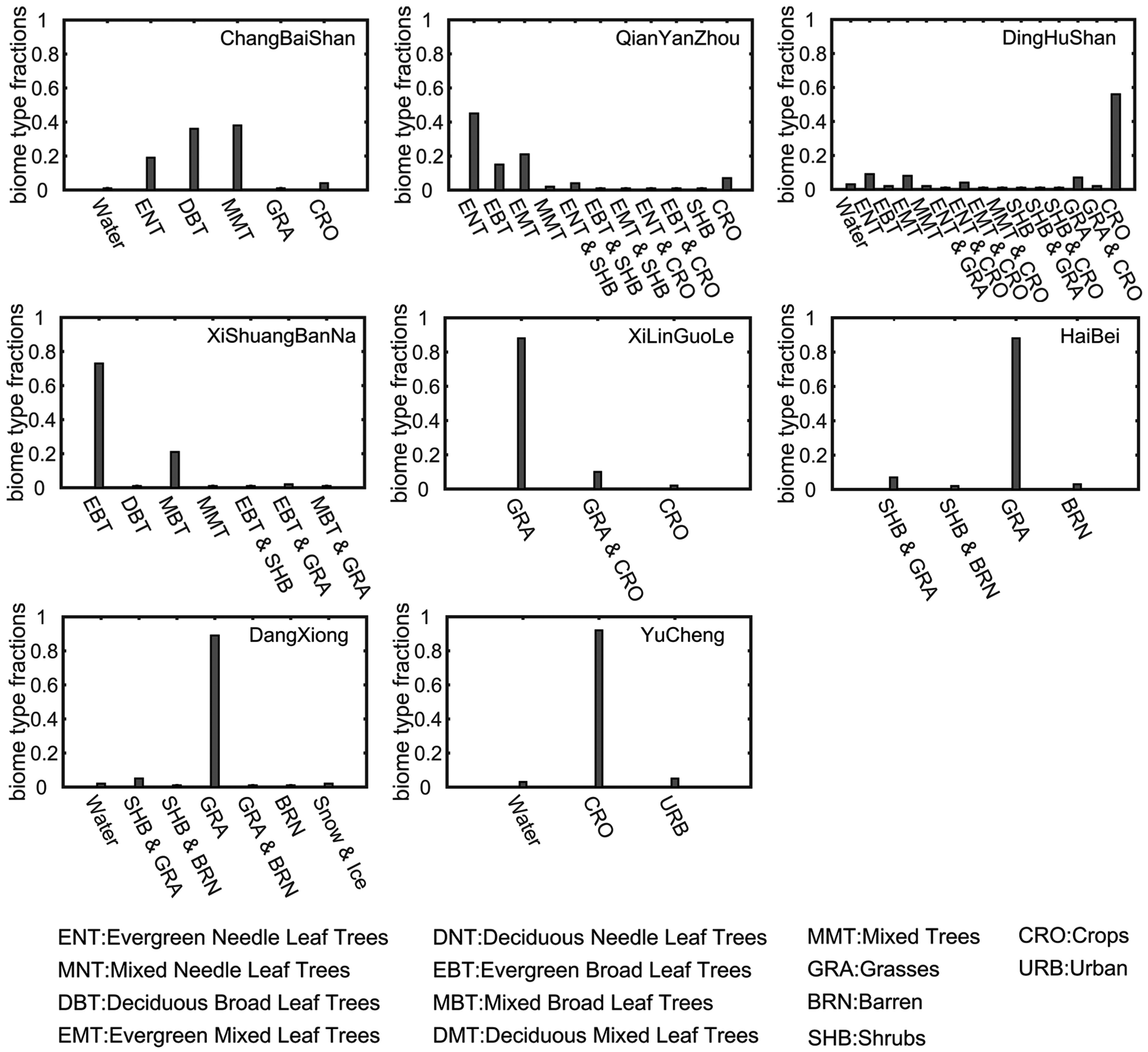 FigureA1. Biome type compositions in the SYNMAP grids corresponding to the ChinaFLUX sites.
Taylor diagrams were used to indicate how well the modeled results matched the observed values in terms of three statistics: the Pearson correlation coefficient (R), the root-mean-square difference (RMSD), and the standard deviation (STD) (Taylor, 2001). The STD and RMSD are proportional to the radial distance from the origin to the observed point. R is defined as the cosine of the azimuth angle. In general, the closer a modeled point is to the observed point, the better the model performs. The Taylor diagrams in Fig. A2 show how closely the GPP from the 14 MsTMIP models matched the observations from 2003 to 2010. The GPP simulations had large uncertainties, especially at YuCheng, where the ground cover was cropland. This means that simple equal-weighted averaging cannot correct the bias when most models have a poor performance for specific PFTs. The diversity in the multi-model results in Fig. A2 shows the need to use a multi-model averaging method that can weight each model according to its simulation skill.
 FigureA2. Taylor diagrams for GPP simulations from 14 MsTMIP models at eight ChinaFLUX sites. The red dashed lines are the observed standard deviations at the sites.
2
APPENDIX A.3 Merging of PFTs when using BMA
When use is made of the observed GPP from ChinaFLUX to train BMA, the dominant PFTs in the qualified grid cells cannot cover all of the PFTs in the SYNMAP legend. To reduce the errors caused by mixed PFTs in the grid cells and the limited number of ChinaFLUX sites, the PFTs at ChinaFLUX sites and used by MsTMIP were categorized as trees, grasses, and crops when BMA was applied. The detailed classifications of the PFTs at ChinaFLUX sites and SYNMAP legend are listed in Table A1 and Table A2, respectively. After being trained by the observed GPP at the grouped ChinaFLUX sites and the MsTMIP GPP in the corresponding grid cells during 2003–08, the weight coefficients of trees, grasses, and crops for different MsTMIP models were calculated by BMA (see Table A3).| SYNMAP legend | BMA classification | ||
| Tree leaf longevity | Tree leaf type | Life form | |
| Evergreen/Deciduous/Mixed | Needle/Broad/Mixed | Trees | Trees |
| Evergreen/Deciduous/Mixed | Needle/Broad/Mixed | Trees & Shrubs | ? Trees, ? Grasses |
| Evergreen/Deciduous/Mixed | Needle/Broad/Mixed | Trees & Grasses | |
| Evergreen/Deciduous/Mixed | Needle/Broad/Mixed | Trees & Crops | ? Trees, ? Crops |
| ? | ? | Shrubs | Grasses |
| ? | ? | Shrubs & Grasses | |
| ? | ? | Shrubs & Crops | ? Grasses, ? Crops |
| ? | ? | Shrubs & Barren | ? Grasses |
| ? | ? | Grasses | Grasses |
| ? | ? | Grasses & Crops | ? Grasses, ? Crops |
| ? | ? | Grasses & Barren | ? Grasses |
| ? | ? | Crops | Crops |
TableA2. Summary of SYNMAP land cover types used for Bayesian model averaging.
| Model Name | Land cover | ||
| Trees | Crops | Grasses | |
| BIOME–BGC | 0.000 | 0.003 | 0.002 |
| CLM4 | 0.000 | 0.000 | 0.005 |
| CLM4VIC | 0.003 | 0.001 | 0.000 |
| DLEM | 0.027 | 0.084 | 0.003 |
| GTEC | 0.001 | 0.005 | 0.013 |
| ISAM | 0.341 | 0.190 | 0.128 |
| LPJ–wsl | 0.000 | 0.003 | 0.002 |
| ORCHIDEE–LSCE | 0.000 | 0.031 | 0.015 |
| SiB3 | 0.564 | 0.594 | 0.011 |
| SiBCASA | 0.034 | 0.071 | 0.001 |
| TEM6 | 0.022 | 0.000 | 0.006 |
| TRIPLEX–GHG | 0.000 | 0.005 | 0.004 |
| VEGAS2.1 | 0.000 | 0.004 | 0.800 |
| VISIT | 0.000 | 0.003 | 0.003 |
TableA3. Weight coefficients for 14 different models calculated by Bayesian model averaging.
2
APPENDIX A.4 Nash–Sutcliffe efficiency index
The Nash–Sutcliffe efficiency index (Ef; Nash and Sutcliffe, 1970) was used to evaluate the performance of the GPP from BMA and individual model in MsTMIP. Its mathematical expression is:where


2
APPENDIX A.5 MODIS GPP and MTE GPP
The monthly MODerate-resolution Imaging Spectroradiometer (MODIS) Version MOD17A2 GPP product (Zhao et al., 2005) was used to evaluate the temporal evolution of the BMA GPP in the target zones. To reduce the disadvantages caused by the difference in spatial resolution (MODIS: 0.05° × 0.05°; MsTMIP: 0.5° × 0.5°) and land cover classification system (MODIS: MOD12Q1; MsTMIP: SYNMAP), we only compared their spatially averaged anomalies from 2000 to 2010.The monthly Model Tree Ensemble (MTE) GPP upscaled from FLUXNET observations to global 0.5° × 0.5° grids during 1982?2010 (Jung et al., 2011) was selected to estimate the magnitude of BMA GPP. Considering that the empirical relationships in machine learning algorithm are time-sensitive, we weakened the time dimension and only compared the spatial patterns of multi-year averaged GPP from MTE, BMA, and MsTMIP to show the rationality of BMA GPP distribution.
