Ning JIANG,
Congwen ZHU^,

Corresponding author: Congwen ZHU,zhucw@cma.gov.cn

State Key Laboratory of Severe Weather and Institute of Climate System, Chinese Academy of Meteorological Sciences, Beijing 100081, China
Manuscript received: 2020-04-03
Manuscript revised: 2020-08-12
Manuscript accepted: 2020-09-10
Abstract:It has been suggested that a warm (cold) ENSO event in winter is mostly followed by a late (early) onset of the South China Sea (SCS) summer monsoon (SCSSM) in spring. Our results show this positive relationship, which is mainly determined by their phase correlation, has been broken under recent rapid global warming since 2011, due to the disturbance of cold tongue (CT) La Ni?a events. Different from its canonical counterpart, a CT La Ni?a event is characterized by surface meridional wind divergences in the central-eastern equatorial Pacific, which can delay the SCSSM onset by enhanced convections in the warming Indian Ocean and the western subtropical Pacific. Owing to the increased Indian?western Pacific warming and the prevalent CT La Ni?a events, empirical seasonal forecasting of SCSSM onset based on ENSO may be challenged in the future.
Keywords: monsoon onset,
SCSSM,
ENSO,
cold tongue La Ni?a,
seasonal forecast
摘要:冬季ENSO暖（冷）事件通常伴随着次年春季南海夏季风的推迟（提前）爆发。我们的研究结果发现，这种相关关系主要是由两者的位相关系决定，而非强度；但是伴随着2011年后全球快速变暖，这种关系被频发的冷舌型La Ni?a事件破坏。与传统的La Ni?a事件不同，这种冷舌型La Ni?a事件主要是由中东太平洋的经向风辐散所主导，能够使副热带西太平洋海温增暖、对流增强，联合印太暖池的增温趋势，进而抑制了南海夏季风的爆发。伴随着印度洋和西太平洋的持续增温，以及冷舌型La Ni?a事件的频发，未来，基于ENSO的南海夏季风爆发的经验预测充满了挑战。
关键词:季风爆发,
南海夏季风,
ENSO,
冷舌型La Ni?a,
季节预测

HTML

--> --> -->

The South China Sea (SCS) summer monsoon (SCSSM) onset generally occurs around 16 May. It has broadly been regarded as the prelude to the East Asian summer monsoon rainy season (Tao and Chen, 1987; Lau and Yang, 1997; Wang et al., 2004; Zhu et al., 2005), and widely concerned in sub-seasonal to seasonal forecasting in China (Zhu and Li, 2017). The crucial physical processes during SCSSM onset are characterized by an eastward extension of the South Asian high in the upper level (He et al., 1987; Liu and Zhu, 2016; Wei et al., 2019), eastward withdrawal of the western North Pacific subtropical high (Xie et al., 1998; Wang et al., 2009), and the generation of convections and cross-equatorial flow over the SCS (Gao and Xue, 2006; Hu et al., 2018).
ENSO has been regarded as the most important factor in the seasonal prediction of the SCSSM onset time on the interannual time scale (Zhou and Chan, 2007; Luo et al., 2016; Luo and Lin, 2017; Martin et al., 2019). According to previous understanding, a warm (cold) ENSO event in winter tends to delay (advance) the onset of the SCSSM by strengthening (weakening) the western North Pacific subtropical high (Zhou and Chan, 2007). On the decadal time scale, warming sea surface temperature (SST) in the equatorial western Pacific can cause earlier SCSSM onset by enhancing intraseasonal variability and tropical cyclone activities (Kajikawa and Wang, 2012), as well as the western Pacific warm pool heat content (Feng and Hu, 2014). However, the onset of the SCSSM has been observed to be relatively late in the past decade, even though the observed SST has kept on warming over the equatorial western Pacific (Luo and Lin, 2017), particularly against a La Ni?a-like SST background (Liu and Zhu, 2019).
In this study, we found that the broken relationship between the SCSSM onset and ENSO can be attributed to the disturbance of cold tongue (CT) La Ni?a events. The prevalent CT La Ni?a events along with the Indian?western Pacific warming in the past decade were able to delay the onset of the SCSSM. Therefore, some previous empirical seasonal forecast models based on ENSO SST indices may fail owing to the recently frequent CT La Ni?a events.

The present study uses monthly and daily SST from the Hadley Centre Sea Ice and Sea Surface Temperature dataset, version 1 (HadISST1), with a 1° × 1° grid (Rayner et al., 2003), and the National Oceanic and Atmospheric Administration (NOAA) High-resolution Blended Analysis of Daily SST (Reynolds et al., 2007). The NOAA interpolated daily outgoing longwave radiation (OLR) (Liebmann and Smith, 1996) and the monthly mean precipitation from the Climate Prediction Center Merged Analysis of Precipitation (CMAP), with a spatial resolution of 2.5° × 2.5° (Xie and Arkin, 1997), are also used. The daily and monthly atmospheric components are taken from the National Centers for Environmental Prediction?National Center for Atmospheric Research (NCEP?NCAR) reanalysis products (Kalnay et al., 1996) from 1948 to present, with a 2.5° × 2.5° horizontal resolution. The mean seasonal cycle from 1981 to 2010 was removed to derive the anomalies for all the variables.
We, following Shao et al. (2015), define the SCSSM onset date by considering both the circulation and convection criteria. Also, the SCSSM onset date anomalies are referred to as the departure from the climatological onset date (16 May; reference line in Fig. 1a). The timing of SCSSM onset based on this definition is nearly consistent to the previous work (Shao et al., 2015), especially for the years to be analyzed (Wang et al., 2004; Liu et al., 2016; Liu and Zhu, 2019). Four ENSO indices (Ni?o 3.4, Ni?o 3, Ni?o 4, Ni?o 1+2) are used to assess the relationship of ENSO diversity with SCSSM onset. Besides Pearson correlation, Spearman (Kendall) Rank correlation—namely, intensity (phase) rank correlation—is used to evaluate the intensity (phase) correlation of ENSO with SCSSM onset. The Spearman Rank (intensity rank) correlation is simply the Pearson correlation coefficient computed using the ranks of the data in intensity. Furthermore, Kendall (phase rank) correlation here is calculated by considering the matching relationship of the data pairs in phases, where the Ni?o indices and the SCSSM onset dates are classified into positive, negative and normal (0) categories.
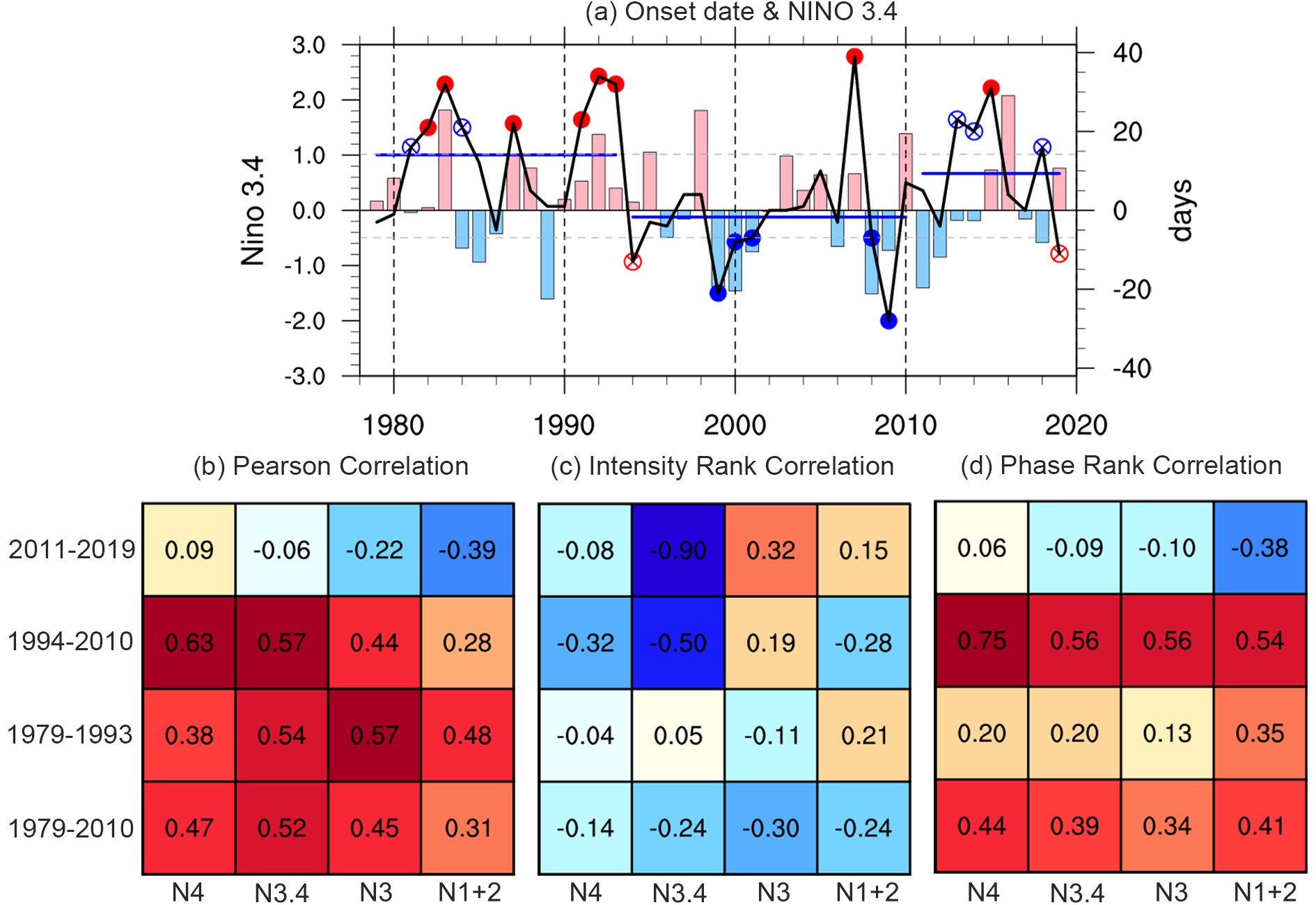Figure1. (a) Time series of SCSSM onset date anomalies and the DJF Ni?o3.4 index (bars). The two horizontal dashed lines represent the averaged values for the late and early onset date anomalies respectively. The SCSSM onset dates exceeding the dashed lines are marked by the dots and circles. The red (blue) dots indicate a late (an early) onset with a positive (negative) Ni?o3.4 index in the previous winter, and instead the others with a reverse relationship are marked by the circles. The blue lines illustrate the averaged onset dates for the periods of 1979?94, 1995?2010 and 2011?19. (b?d) Correlation coefficients between four ENSO indices and SCSSM onset date during the three periods. The Pearson correlation, Intensity Rank correlation and Phase Rank correlation are illustrated in (b?d) respectively.

The SCSSM onset shows a decadal variability, characterized by alternating late-onset [1979?93 (P1) and 2011?19 (P3)] and early-onset [1994?2010 (P2)] periods during recent decades. The interdecadal change between P1 and P2 has been discussed in several studies (Kajikawa and Wang, 2012; Feng and Hu, 2014; Chen, 2015). It is suggested that the relationship between SCSSM onset and ENSO varies on the decadal time scale (Wang et al., 2013; Ding et al., 2016; Liu et al., 2016). To examine whether or not the relationship between ENSO and SCSSM onset is stable, we calculated the correlations of the SCSSM onset anomaly with four ENSO SST indices (Ni?o 4, Ni?o 3.4, Ni?o 3 and Ni?o 1+2) in the previous winter (Fig. 1). The positive correlation during P2 is more notable than that during P1 (Fig. 1b), which seems to be attributable to the Atlantic Multidecadal Oscillation or Pacific Decadal Oscillation (e.g., Ding et al., 2016; Liu et al., 2016; Wang et al., 2017). However, the Pearson correlations of SCSSM onset with all Ni?o indices drop significantly during P3, suggesting the traditionally positive relationship between ENSO and SCSSM onset has been broken in the past decade.
The Pearson correlation between the SCSSM onset and ENSO indices is a result combining the mutual relationship of the intensities and phases between the two time series. The positive Pearson correlations between the SCSSM onset and ENSO indices during the period before 2010 (Fig. 1b) are mainly contributed by their phase correlation (Fig. 1c), instead of the intensity correlation (Fig. 1d). This implies that the influences of ENSO on SCSSM onset are mainly determined by the spatial pattern of El Ni?o-like or La Ni?a-like SST anomalies (SSTAs) instead of the amplitude of ENSO indices (extreme or moderate). It is noted that the warm phase of ENSO is mostly followed by late SCSSM onset during the whole period of 1979?2019, but the cold phase of ENSO can be followed by either earlier or late onset (Fig. 1a). It has been suggested that the notable positive correlation between ENSO and SCSSM onset during the early-onset period (P2) can be attributed to the frequent La Ni?a events (Liu et al., 2016). However, the three cold events (2013, 2014 and 2018) during P3, corresponding to the negative phase of ENSO, are all followed by late SCSSM onset. This suggests that the broken positive correlation between ENSO and SCSSM onset during P3 is possibly contributed by the negative phase of ENSO in the past decade.
To verify our hypothesis, we investigate five La Ni?a-like events (1999, 2000, 2001, 2008 and 2009) followed by notable early SCSSM onsets for comparison, and try to reveal the distinct impacts of cold ENSO between P2 and P3. Their composite SSTAs in the previous winter (DJF; December?January?February) resemble the canonical La Ni?a pattern (Fig. 2a) along with strengthened pan-tropical Pacific Walker circulation and enhanced convection over the SCS (Fig. 2b). Two opposite anomalous vertical circular circulation centers are located over the west and east of the SCS (Fig. 2b) with strong low-level zonal wind convergence over the SCS (Fig. 2a). The central-eastern Pacific cooling is likely related to the Bjerknes feedback, which emphasizes the role of the zonal wind in air?sea interaction.
Figure2. (a) DJF SST (shading), 10-m wind (vectors) and precipitation anomalies (contours; blue: positive, red: negative), and (b) zonal mass stream function, pressure velocity (omega × ?50; units: Pa s^?1), and zonal divergent wind (units: m s^?1) averaged within 5°S?5°N for the composite of La Ni?a events (1999, 2000, 2001, 2008 and 2009). The second, third and fourth rows represent those in 2013, 2014 and 2018 (precipitation anomalies: contours with crossing lines; 2 mm d^?1 interval). Only the values for the wind and SST (precipitation) anomalies above the 90% confidence level are shown (marked by dots) in (a). The white boxes in (a) and (c, e, g) represent the areas (5°S?5°N, 150°E?150°W and 2.5°S?2.5°N, 170°W?120°W) that define the ${U_{\rm{w}}}$ and ${\rm{M}}{{\rm{D}}_{\rm{c}}}$ indices, respectively. (i) Scatterplot of ${U_{\rm{w}}}$ and ${\rm{M}}{{\rm{D}}_{\rm{c}}}$ for winters (DJF) from 1979 to 2019. Blue dots represent the La Ni?a events followed by early SCSSM onset. The 2013, 2014 and 2018 cases with late SCSSM onset are shown as red dots. (j) Time series of DJF Ni?o3.4 index: observations (gray); linear regression with the residual ${\rm{M}}{{\rm{D}}_{\rm{c}}}$ as the only predictor (red); and linear regression with both the ${U_{\rm{w}}}$ and residual ${\rm{M}}{{\rm{D}}_{\rm{c}}}$ indexes as predictors (blue).


Although the three cold events (2013, 2014 and 2018) in P3 share a roughly similar anomalous SST morphology in P2 as the canonical La Ni?a events, the detailed atmospheric circulation structures are quite different (Figs. 2c-h vs. Figs. 2a and b). The cooling areas in the east of the tropical Pacific for the three events are much narrower in the meridional direction (white boxes in Figs. 2c, e and g) along the equator, and their zonal trade wind anomalies around the dateline are much weaker. The equatorial narrow cooling in the three La Ni?a events is closely related to the surface meridional wind divergence instead of the zonal trade wind. In addition, the associated convections surrounding the eastern cooling regions are located in the western Pacific and north and south subtropical Pacific (Figs. 2c, e and g). Compared with the canonical La Ni?a events in Figs. 2a and b, the convections in the recent three cold events are much weaker and located in the east of the SCS. Correspondingly, a strong vertical circular circulation is located to the east of 150°E. Some scattered convections around the SCS also induce several reversed vertical circular circulations, but seem irrelevant to the large-scale Pacific Walker circulation (Figs. 2d, f and h). Considering the common unique features of the three cold events, these La Ni?a-like events along with surface meridional wind divergence and narrow east cooling resembles the so-called CT mode (Zhang et al., 2010; Li et al., 2015; Jiang and Zhu, 2018, 2020)—namely a background mode under recent global warming. Therefore, these cold events in P3 can be named as CT La Ni?a events. However, it is hard to distinguish these CT La Ni?a events from the canonical La Ni?a events based only on the current SST Ni?o indices. Thus, a new index is introduced to depict the CT La Ni?a events.
Considering the surface wind features of CT La Ni?a events, the surface meridional wind divergence $\left( {{\partial v}}/{{\partial y}}\right)$ averaged within the box in Fig. 2c—namely, ${\rm{M}}{{\rm{D}}_{\rm{c}}}$ index—is used to depict the variation related to the CT La Ni?a events. However, the strengthened zonal winds for the canonical La Ni?a events within the box (${U_{\rm{w}}}$ index) in Fig. 2a can also induce meridional wind divergence sometimes (Fig. 2i). On the other hand, compared with canonical La Ni?a events followed by early SCSSM onsets (marked with blue dots), the zonal trade winds (${U_{\rm{w}}}$) in the CT La Ni?a events (marked with red dots) are much weaker. It seems that both strengthened zonal trade winds and the surface meridional wind divergence can lift the thermocline and cool the SST in the eastern Pacific. To address the CT La Ni?a dominated by ${{\partial v}}/{{\partial y}}$, the residual ${\rm{M}}{{\rm{D}}_{\rm{c}}}$ is obtained by linearly removing the influence of the ${U_{\rm{w}}}$ index. Figure 2j illustrates the time series of the observed Ni?o3.4 index and that regressed on the residual ${\rm{M}}{{\rm{D}}_{\rm{c}}}$ and the combination of the residual ${\rm{M}}{{\rm{D}}_{\rm{c}}}$ and ${U_{\rm{w}}}$ index. Results show that Ni?o3.4 index regressed on the combination of the residual ${\rm{M}}{{\rm{D}}_{\rm{c}}}$ and ${U_{\rm{w}}}$ index gives a times series more correlated with the observed Ni?o3.4 index [mean squared error (MSE): 0.12] than that regressed on the residual ${\rm{M}}{{\rm{D}}_{\rm{c}}}$ alone (MSE: 0.67). However, the Ni?o3.4 indices of the three CT La Ni?a events are reproduced well by the residual ${\rm{M}}{{\rm{D}}_{\rm{c}}}$(MSE: 0.016) in the past decade, suggesting a dominant role of the meridional wind divergence in inducing eastern Pacific cooling in the recent three CT La Ni?a events. Therefore, the residual ${\rm{M}}{{\rm{D}}_{\rm{c}}}$ is used as an index to depict the CT La Ni?a events. Since there are distinct differences between the CT La Ni?a events and the canonical ones, their impacts on the pre-onset stage of the SCSSM onset are further examined.

The persistence of SSTAs and the circulation patterns from the previous winter to spring may maintain the ENSO?SCSSM linear relationship and favor the seasonal forecasting of SCSSM onset (Figs. 3a-f). Figure 3 shows the temporal evolution of air?sea anomalies (OLR and SSTA) before the SCSSM onset for each cold event during P2 and P3. The five La Ni?a events followed by early SCSSM onsets in P2 exhibit persistent enhanced convection over the SCS from winter to spring (April), favoring early onset of the SCSSM (marked by black circles in Figs. 3a-f). In contrast, no obvious persistence of enhanced convection signals is observed in the SCS following the CT La Ni?a events in P3, and the suppressed convections over the SCS in May postpone the onset of the SCSSM.
Figure3. Hovm?ller diagrams for OLR (shading) and SST (contours; red: positive, blue: negative) anomalies averaged within the tropical band (10°?20°N) for composited (f) and individual cases. Panel (f) represents the case composited by (a?e). The horizontal and vertical reference lines represent the climatological SCSSM onset date and the SCS position. The yellow stars indicate the SCSSM onset dates for different years, and the evolutions of convection around SCSSM onset are marked by the black circles.


Consistent with the persistence of convection over the SCS, the air?sea structures of the canonical La Ni?a events during P2 also persist from winter to spring (Figs. 4a-c). However, the structures of the CT La Ni?a events change greatly in spring. An evident anomalous anticyclone (marked by the letter “A” in the left-hand column in Fig. 4) in the lower troposphere is centered over the SCS with suppressed convection, which possibly postpones the SCSSM onset. The enhanced convections surrounding the SCS are mainly located over the northern Indian Ocean, Maritime Continent, and western Pacific (150°E?180°), inducing vertical circular circulations influencing the SCSSM onset. For instance, in May 2013, the enhanced convections over the Maritime Continent and northern Indian Ocean induce strong descending motion over the SCS (second row in Fig. 4). Besides the convections over the Maritime Continent and northern Indian Ocean, the enhanced convections over the northern subtropical Pacific also suppress the convections over the SCS in 2018 (last row in Fig. 4).
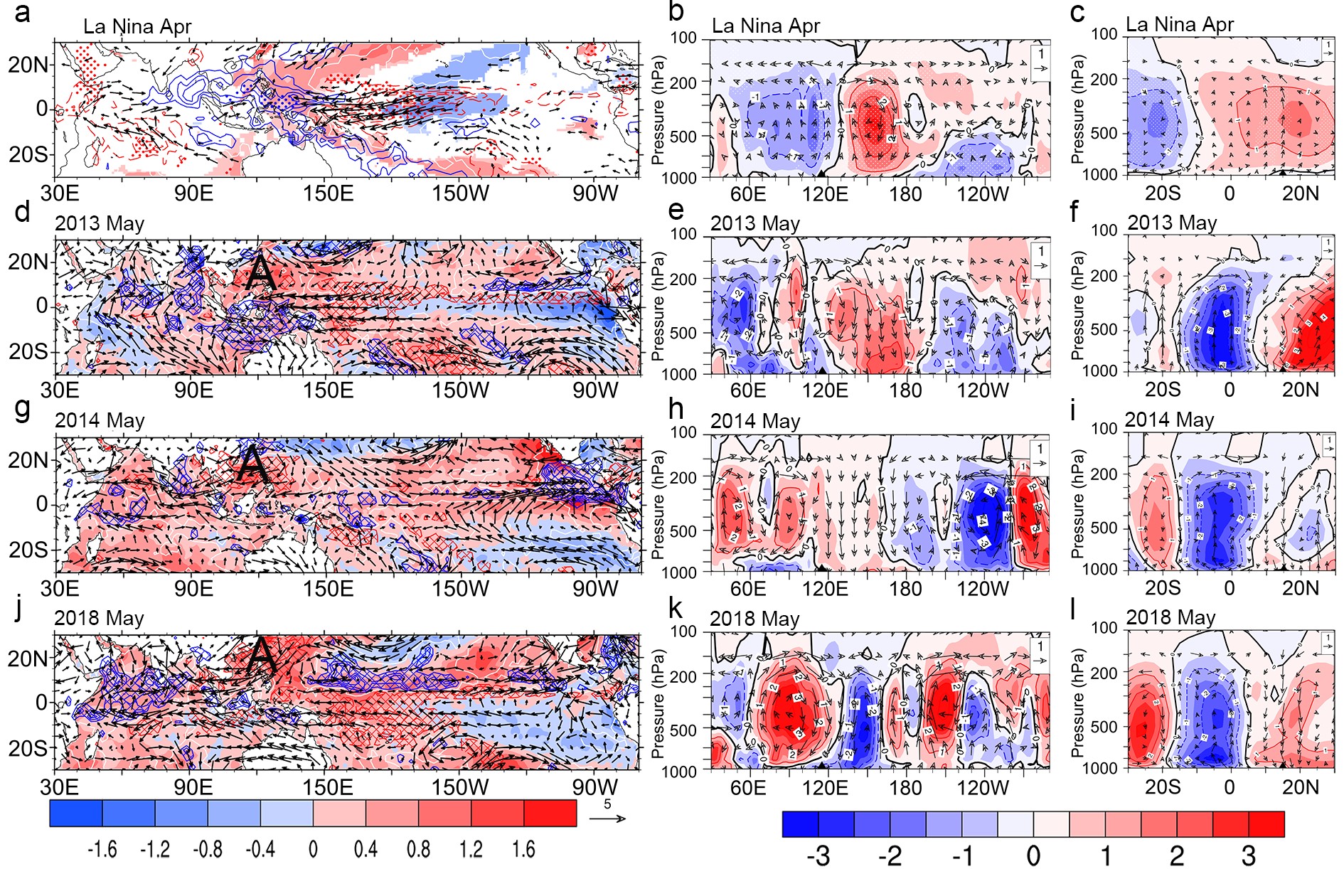Figure4. Similar to Fig. 2 but for (a) SST (shading), 10-m wind (vector) and precipitation (contours; blue: positive, red: negative) anomalies, (b) zonal mass stream function, pressure velocity (omega × ?50; units: Pa s^?1), and zonal divergent wind (units: m s^?1) averaged within 10°?20°N, and (c) meridional mass stream function, pressure velocity (omega × ?50; units: Pa s^?1), and meridional divergent wind (units: m s^?1) averaged within 110°?120°N for the composited La Ni?a case in May. The second, third and fourth rows represent those in 2013, 2014 and 2018. The location of the SCS is marked by the black triangle in the last two rows.


According to the above analyses, the canonical La Ni?a events in P2 strengthen the pan-tropical Pacific Walker circulation, enhance persisting convection over the SCS, and advance the SCSSM onset, supporting the positive relationship between SCSSM onset and ENSO. In contrast, the CT La Ni?a events in P3 induce a vertical circular circulation over the east of the SCS, but it cannot maintain to spring. The late onset of the SCSSM following the CT La Ni?a years in P3 is mainly postponed by enhanced convections over the northern Indian Ocean, Maritime Continent, and western Pacific surrounding the SCS.
To further verify the impact of CT La Ni?a on late SCSSM onset, we firstly remove the influence of the zonal wind (${U_{\rm{w}}}$), and then indicate the variations of the CT La Ni?a events by the DJF residual ${\rm{M}}{{\rm{D}}_{\rm{c}}}$ index. By regressing the SSTAs on the DJF residual ${\rm{M}}{{\rm{D}}_{\rm{c}}}$ index, the winter (DJF) SSTA pattern resembles that of the three CT La Ni?a events, characterized by a narrow cooling in the eastern equatorial Pacific along with significant meridional wind divergence (Fig. 5a). In addition, there is slight cooling over the Indian Ocean and the oceans surrounding the Maritime Continent.
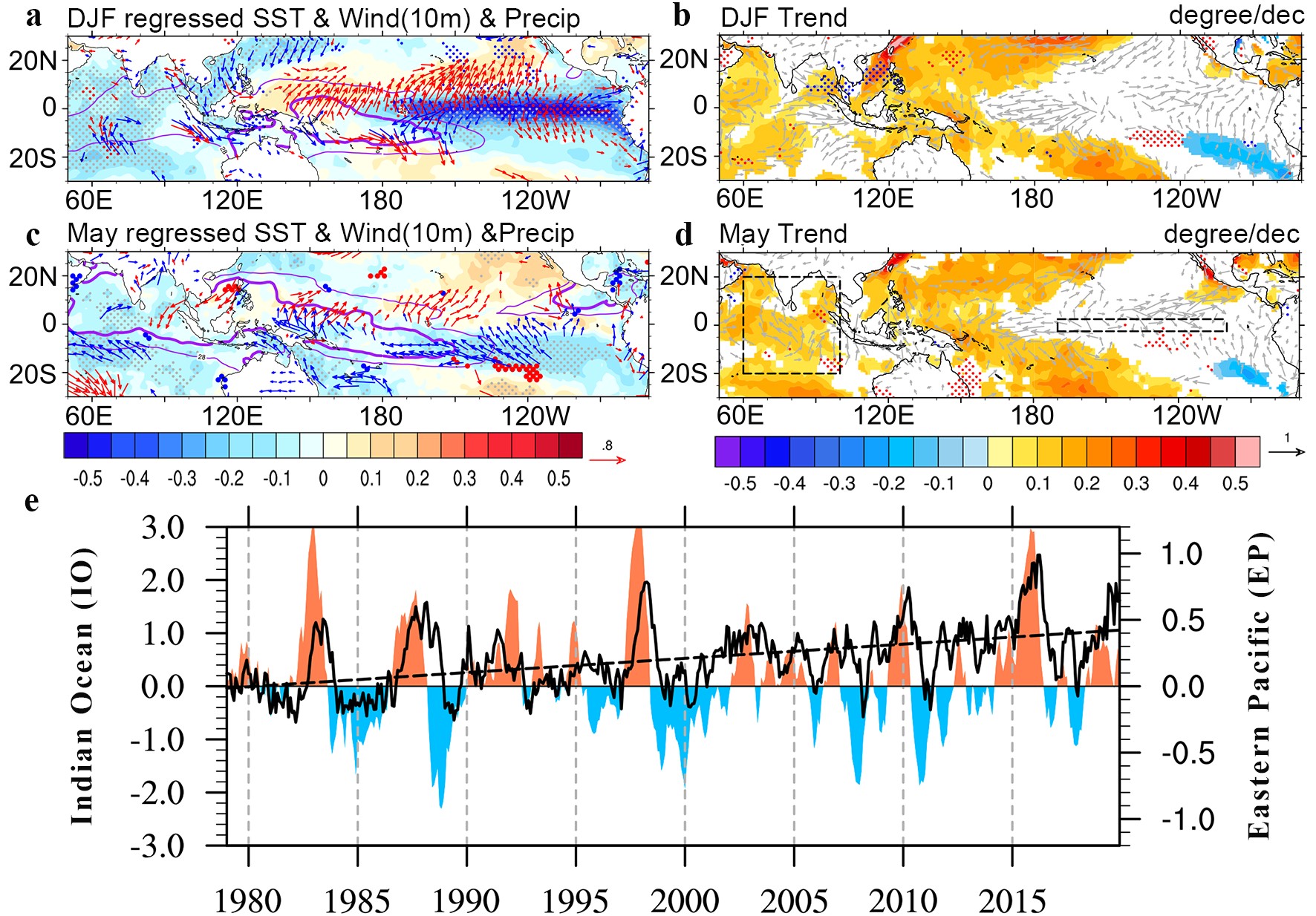Figure5. (a) The DJF residual ${\rm{M}}{{\rm{D}}_{\rm{c}}}$-regressed (a) DJF and (c) May SSTA spatial distribution (shading; 0.05 K interval), horizontal wind at 10 m (vectors), and precipitation (dots; mm d^?1). The blue (red) dots indicate the positive (negative) precipitation anomalies. The surface wind anomalies stronger (weaker) than the climatological winds are in blue (red). The thin and thick purple lines indicate the climatological 28°C and 29°C isotherms in (a) DJF and (c) May. (b, d) Trends in SST [units: °C (10 yr)^?1], 10 m winds [arrows; units: m s^?1 (10 yr)^?1], and precipitation (blue dots: positive, red dots: negative) for (b) DJF and (d) May. (e) SSTA averaged within the Indian Ocean (black solid line) and eastern Pacific (blue and red shading) regions [marked in (d) by dashed line boxes (20°S?20°N, 60°E?120°E and 2.5°S?2.5°N, 170°W?100°W) ] in which the dashed line indicates the linear trend for the time series of the Indian Ocean SSTA.


The warming Indian Ocean?western Pacific and the cooling along the coast of Peru in the CT La Ni?a events during P3 are mainly contributed by their trends under global warming (Fig. 5b). Also, the northern and southern subtropical Pacific are warming significantly via the wind?evaporation?sea surface temperature feedback (Fig. 5a). Considering the seasonal march of the warm pool regions (purple lines in Figs. 5a and c) and the evolution of CT La Ni?a, the convections over the SCS should be suppressed thanks to the surrounding enhanced convections, particularly over the Indian Ocean and the northern subtropical Pacific.
Besides the interannual variation, the warming trend of the Indian Ocean is also significant. Although the Indian Ocean Capacitor effect (Xie et al., 2009) after ENSO can still be detected by the phase-lag relationship of SSTAs between the eastern Pacific and Indian Ocean (Fig. 5e), the SSTA barely cools owing to the rapid warming in the Indian Ocean in the past decade, suggesting an asymmetrical response of the Indian Ocean SSTA to ENSO. For the three CT La Ni?a events during P3, the warming surrounding the SCS could have enhanced convections and postponed the SCSSM onset. Since SCSSM onset can also be triggered by synoptic or intraseasonal activities, the warming SST in the Indian Ocean can enhance convection and atmospheric disturbance and in turn bring greater uncertainties for the seasonal forecasting of SCSSM onset. Following an El Ni?o event, the warming SSTA may become remarkable in the Indian Ocean and result in enhanced convection disturbances to trigger an early onset of the SCSSM. For example, the extreme early SCSSM onset in 2019 was attributed to the intraseasonal oscillation (Hu et al., 2020) and typhon “Fani” (Liu and Zhu, 2020). Liu and Zhu (2020) indicated that the anomalous condensation heating released by the typhon not only shifted the South Asian high northward, but also reinforced the upper-level barotropic trough to the west of the Tibetan Plateau at midlatitudes. This facilitated the early establishment of monsoon convection by intensifying the upper-level pumping over the SCS.

ENSO has been treated as the most important predictor for SCSSM onset in empirical and dynamical models (Zhu and Li, 2017; Martin et al., 2019). A warm (cold) ENSO event is often followed by late (early) onset of the SCSSM. However, this positive correlation does not work during 2011?19. Our results show that the anomaly of SCSSM onset is mainly determined by the phases (warm or cold) of ENSO, instead of the amplitude of the anomalous SST index. The recent invalid positive correlation between SCSSM onset and ENSO can be attributed to the disturbance of CT La Ni?a events during 2011?19.
The anomalous SST morphology of CT La Ni?a resembles that of conventional events, but its cooling area is narrowed along the equator with weaker trade winds. We found that the cooling SST of CT La Ni?a events is dominated by the meridional wind divergence in the eastern Pacific, which is distinct from canonical La Ni?a events with strong trade winds. Following a CT La Ni?a in the preceding winter, the suppressed convections over the SCS in May postpone the SCSSM onset, which is mainly due to the enhanced convections over the northern Indian Ocean, western Pacific, and Maritime Continent. It is suggested that both the evolution of CT La Ni?a and the warming SST in the Indian?western Pacific contribute to late SCSSM onset.
CT La Ni?a events dominated by surface meridional wind divergence have been more likely to occur in recent years, but can barely be distinguished from canonical events by the SST ENSO indices alone. Due to the distinct influences of CT La Ni?a events, some known empirical seasonal forecast models based on ENSO SST indices may be challenged. Therefore, besides these SST ENSO indices, it is suggested that additional indices, such as ${U_{\rm{w}}}$ and ${\rm{M}}{{\rm{D}}_{\rm{c}}}$, are also used to monitor ENSO diversity for the seasonal forecasting of SCSSM onset. The increasing frequency of CT La Ni?a events may also affect the diversity of ENSO, including the SST patterns and evolutions. Hence, more studies should be carried out with the aim to better understand CT La Ni?a events.
Acknowledgements. The authors acknowledge the anonymous reviewers’ helpful suggestions, and Dr. Jeremy Cheuk-Hin LEUNG’s polishing. This work was jointly sponsored by the National Key R&D Program (Grant No. 2018YFC1505904), the National Science Natural Foundation of China (Grant No. 41830969) and the Basic Scientific Research and Operation Foundation of the Chinese Academy of Meteorological Sciences (Grant Nos. 2018Z006 and 2018Y003), and the scientific development foundation of CAMS (2020KJ012). This study was also supported by the Jiangsu Collaborative Innovation Center for Climate Change. The HadISST1 dataset was obtained from the Met Office Hadley Centre and can be downloaded from http://www.metoffice.gov.uk/hadobs/hadisst/data/download.html. The NOAA High-resolution Blended Analysis of Daily SST, NCEP reanalysis data, interpolated OLR data, and CMAP precipitation data, provided by NOAA/OAR/ESRL PSD, Boulder, Colorado, USA, can be obtained from their website at https://www.esrl.noaa.gov/psd/.