Masakazu TAGUCHI^,

Corresponding author: Masakazu TAGUCHI,mtaguchi@auecc.aichi-edu.ac.jp

Department of Earth Science, Aichi University of Education, Kariya 448-8542, Japan
Manuscript received: 2019-09-14
Manuscript revised: 2019-11-18
Manuscript accepted: 2019-12-02
Abstract:This study reports verification results of hindcast data of four systems in the subseasonal-to-seasonal (S2S) prediction project for major stratospheric sudden warmings (MSSWs) in northern winter from 1998/99 to 2012/13. This report deals with average features across all MSSWs, and possible differences between two MSSW types (vortex displacement and split types). Results for the average features show that stratospheric forecast verifications, when further averaged among the four systems, are judged to be successful for lead times around 10 d or shorter. All systems are skillful for lead times around 5 d, whereas the results vary among the systems for longer lead times. A comparison between the MSSW types overall suggests larger forecast errors or lower skill for MSSWs of the vortex split type, although the differences do not have strong statistical significance for almost all cases. This limitation is likely to at least partly reflect the small sample size of the MSSWs available.
Keywords: major stratospheric sudden warmings,
forecast verification,
subseasonal-to-seasonal prediction project,
vortex displacement and split warmings
摘要:基于回报试验结果，这个研究工作对四个预报系统进行的1998/99-2012/13年冬季北半球平流层爆发性增温(MSSWs)的次季节至季节预报方案进行了验证。本研究讨论了所有MSSWs的平均特征，以及两种MSSWs类型（极涡位移型和极涡分裂型）之间可能存在的差异。平均特征表明，当对四个系统的结果进行平均处理时，可以成功地超前10天或更短一点时间的预报MSSWs。另外，每个系统超前5天的预报技巧都很高，但是对于更长的预报时间，各个系统的预报能力有所不同。对比不同类型的MSSWs的预报结果发现，对极涡分裂型MSSWs的预报会存在较大误差并且预报技巧较低。所有事件中这些差异在统计检测中并不显著，这种差异的不显著可能与个例太少有很大的关系。
关键词:平流层爆发性增温,
预报验证,
次季节至季节预报方案,
极涡位移与极涡分裂

HTML

--> --> -->

Extreme states in the northern extratropical stratosphere during its winter have been receiving a lot of attention, especially since some of them have been discovered to propagate downward to the troposphere and accompany anomalous weather conditions there (e.g., Baldwin and Dunkerton, 2001). The winter stratosphere is usually characterized by the cyclonic vortex encompassing the polar region, called the stratospheric polar vortex (Waugh et al., 2017). The polar vortex sometimes largely distorts and even breaks down accompanying sharp and large temperature increases in the polar stratosphere (Andrews et al., 1987); these are called stratospheric sudden warmings (SSWs), and a prominent example of such stratospheric extreme states accompanying anomalous weather conditions.
Some SSWs are referred to as major SSWs (MSSWs), e.g., when the zonal mean zonal wind at (60°N, 10 hPa) reverses from a westerly wind to an easterly wind (Charlton and Polvani, 2007; Butler et al., 2017). SSWs are also classified into either vortex displacement (VD) or vortex split (VS) types (Charlton and Polvani, 2007). The polar vortex shifts away from the pole without a split during VD MSSWs, whereas it splits into two during VS MSSWs. VD and VS MSSWs are associated with intensification of the planetary wave of zonal wavenumber 1 (wave 1) and 2 (wave 2), respectively.
The importance of extreme stratospheric states in tropospheric weather forecasts has been recognized especially for medium-range and seasonal time scales. Sigmond et al. (2013) demonstrated higher forecast skill for near-surface weather variables for about two months when the forecasts are initialized on observed MSSW onset dates, compared to unconditional forecasts. A similar result was obtained by Tripathi et al. (2015a), who analyzed European Centre for Medium-Range Weather Forecasts (ECMWF) hindcast (HC) data focusing on anomalously strong states of the stratospheric polar vortex. Scaife et al. (2016) suggested that occurrence of MSSWs contributes to the high correlation of their seasonal forecast experiments for the winter North Atlantic Oscillation.
A surge of recent studies have also been investigating the predictability of MSSWs, partly motivated by the recognition of the stratospheric importance (Tripathi et al., 2015b). In particular, Taguchi (2016a) extracted average features and case-to-case variations of MSSW forecasts by analyzing Japan Meteorological Agency (JMA) one-month forecasts (see also Karpechko, 2018; Domeisen et al., 2019; Rao et al., 2019a). Taguchi (2016b, c) further contrasted forecasts for VD and VS MSSWs in JMA HC data to argue for greater difficulty (larger errors) in forecasting VS MSSWs and associated wave activity.
A few other studies have tackled this issue (i.e., possible differences in forecast skill between VD and VS MSSWs), and support the result. Analyzing China Meteorological Administration (CMA) HC data for a few VS MSSWs, Rao et al. (2018) suggested that this result also holds for the CMA data. A case study by Taguchi (2018) using the subseasonal-to-seasonal (S2S) data archive (Vitart et al., 2017) compared two VD and two VS MSSWs in northern winter for a consistent result. On the other hand, in his analysis of ECMWF HC data, Karpechko (2018) was cautious about drawing a firm conclusion on this issue because of the limited sample size.
The present study seeks to further explore stratospheric predictability features for MSSWs in northern winter in terms of average features across MSSWs and differences between VD and VS MSSWs. A main motivation is that most of the abovementioned studies were based on single systems. This study intends to report results from a multi-system comparison using the S2S data archive for multiple (about 10) MSSWs. It deals with MSSWs from 1998/99 to 2012/13 that are available to HC data of four S2S systems providing relatively abundant data. As far as verifications for MSSW forecasts during December–January–February (DJF) are concerned, the present report is more comprehensive than Domeisen et al. (2019) in terms of verification measures and MSSW classifications.
The rest of the paper is organized as follows: section 2 documents the data and analysis method in this study; sections 3 and 4 report average features and variability among MSSWs, respectively; and finally, section 5 provides a summary and discussion.

2

-->

2.1. Japanese 55-year Reanalysis data

Daily averages of the Japanese 55-year Reanalysis (JRA-55) data (Kobayashi et al., 2015) are used as a representation of the real world when the S2S HC data are verified in this study. The JRA-55 data period for this study is from January 1979 to June 2018, extending for 40 northern winter seasons from 1978/79 to 2017/18.
Onset dates of MSSWs are identified in the JRA-55 data during DJF, and 22 cases for the 40 seasons are obtained (Table 1). The MSSW onset dates are basically identified as reversals of the zonal mean zonal wind [U] at (60°N, 10 hPa) (Charlton and Polvani, 2007). Here, the square brackets denote the zonal mean. All onset dates are identical to the results obtained by Butler et al. (2017) for the JRA-55 data, except for the MSSW #22 that occurred in February 2018. Another MSSW occurred in the 2018/19 winter season (Rao et al., 2019b), but is not included here as it is outside the 40-season period of interest. The onset dates are also referred to as lag = 0 d.

Number #	Onset date	Wave 2 amplitude	Aspect ratio	Karpechko
1	1979/02/22	S	S	S
2	1980/02/29	D	D	D
3	1981/02/06	S	D	D
4	1981/12/04	D	D	D
5	1984/02/24	D	S	D
6	1985/01/01	S	S	S
7	1987/01/23	S	D	D
8	1987/12/08	D	D	S
9	1989/02/21	S	S	S
10	1998/12/15	D	D	D
11	1999/02/26	S	S	S
12	2001/02/11	D	S	S
13	2001/12/31	D	S	D
14	2003/01/18	S	S	S
15	2004/01/05	D	D	D
16	2006/01/21	S	D	D
17	2007/02/24	D	D	D
18	2008/02/22	D	D	D
19	2009/01/24	S	S	S
20	2010/02/09	D	S	S
21	2013/01/07	S	S	S
22	2018/02/12	S	D	S

Table1. MSSW onset dates (yyyy/mm/dd format) identified for DJF in the JRA-55 data. Each MSSW is classified into the VD (D) or VS (S) type using three methods.


Each MSSW is further classified as either VD or VS type using three methods (Table 1). The first method uses the amplitude of wave 2 in the JRA-55 10 hPa geopotential height (Z10) field at 60°N around each MSSW onset date (lag = ?2 to +2 d). An MSSW is classified as a VS MSSW if the wave 2 amplitude is equal to or larger than the median of the 22 values (i.e., for the 22 MSSWs), and the rest are VD MSSWs (Fig. 1). The second method similarly uses the aspect ratio of the 5 d mean Z10 around each onset date (Seviour et al., 2013). The last method follows the result from Karpechko et al. (2017) after Lehtonen and Karpechko (2016), except for #3, #21, and #22. These studies look for two separate minima in Z10. The three MSSWs are not included in these studies, and are judged from the JRA-55 Z10 field subjectively. The method based on the wave 2 amplitude is used to demonstrate example results below.
Figure1. (a) Scatterplot between the wave 1 and wave 2 amplitudes of the 10 hPa height Z10 at 60°N for all 22 MSSWs in the JRA-55 data. The Z10 field is averaged for 5 days (lag = ?2 to +2 d) around each MSSW onset date. The best-fit line and correlation coefficient for the 22 MSSWs are indicated. The filled markers are for the MSSWs #10–#21 covered by the ECMWF HC data, and are colored according to the RMSE of the ECMWF LTG-15 forecasts (see the colorbar). Panel (b) is similar, but uses the centroid latitude and aspect ratio of the 5 d averaged Z10 field.



2 -->

2.2. S2S HC data

From the S2S data archive, this study employs HC data of the four systems of BoM, CMA, ECMWF, and NCEP (Table 2). The four systems are chosen because they provide relatively abundant data in terms of initialization frequency and ensemble size (Vitart et al., 2017). HC data are obtained that were initialized from November to February since northern winter is the focus in this study. The different systems cover different MSSWs. The present analysis uses 12 MSSWs (#10–#21) for a fair comparison that are commonly covered by three of the four systems, except for NCEP. For NCEP, the MSSWs #11–#20 are examined.

System name	Period	Initialization frequency	Ensemble size	MSSWs covered
BoM (Australian Bureau of Meteorology)	1981–2013	Six per month	11**	#3–#21
CMA (China Meteorological Administration)	1994–2014	Daily	4	#10–#21
ECMWF* (European Centre for Medium-Range Weather Forecasts)	1997 (November)–2017 (February)	Two per week	11	#10–#21
NCEP (National Centers for Environmental Prediction)	1999–2010	Daily	4	#11–#20
*The ECMWF HC data in the S2S archive are performed for an “on-the-fly” mode, whereas the three others use a “fixed” mode. The ECMWF HC data used in this study are those associated with real-time forecasts for the 2017/18 northern winter season. **This study uses 11 members of BoM for each initial date to facilitate the download and analysis, whereas 33 members are available. A preliminary analysis indicated that 11 members of BoM are sufficient for the present purpose.

Table2. Four S2S systems employed in this study.


The HC data analyzed here can be simply expressed for any quantity of interest, A, for each HC set (ensemble forecasts initialized on a day) as A_{HC_set} (forecast time, ensemble member). Each forecast set is determined by its initial date and forecast system. Spatial information is omitted here for simplicity.
For each MSSW and system, the HC data are further organized into four lead-time groups (LTGs) of LTG-20, LTG-15, LTG-10, and LTG-5 to facilitate a comparison among different MSSWs and systems, e.g., as in Taguchi (2018), Rao et al. (2018), and Domeisen et al. (2019). For example, the LTG-15 for each MSSW and system combines all available HC data of the system initialized from lag = ?15 to ?11 d of the target MSSW (Fig. 2). The HC data in each LTG are sorted in time lag with respect to the MSSW onset date as A_LTG-i (time lag, ensemble member). Here, the ensemble size of A_LTG-i may increase from that of A_{HC set} when multiple initial dates are available for the LTG. Then, the JRA-55 and HC data around the observed MSSW onset dates are compared (Fig. 2). The possible effects of different initialization frequencies and ensemble sizes among different LTGs, MSSWs, and systems are not considered. The HC data are not bias-corrected in order to examine their intrinsic forecast skill, although bias corrections might lead to improved MSSW forecasts (Rao et al., 2019a). We use ensemble means for each A_LTG-i for most verifications, unless stated otherwise.
Figure2. Schematic showing the analysis procedure for the forecast verification using the MSSWs (lag = 0 d) as a key. This figure uses LTG-15 as an example.


The forecast verification employs the following measures:
(1) Zonal mean zonal wind [U] at (60°N, 10 hPa) around the MSSW onset dates (averaged from lag = ?2 to +2 d). The HC zonal wind data around the onset dates are roughly equivalent to zonal wind errors (differences from the JRA-55 data), since the JRA-55 counterpart can be approximated as zero.
(2) Hit rate (HR). This is defined as a ratio (in percentage) of the number of successful ensemble members to the ensemble size for each LTG, MSSW, and system. The successful ensemble members are those that show a reversal of [U] at (60°N, 10 hPa) for the first time between lag = ?3 to +3 d, i.e., a 3 d difference is allowed between the observed and HC onset dates. This measure was introduced in Taguchi (2016a) to verify MSSW forecasts and was used, for example, in Rao et al. (2018) and Domeisen et al. (2019).
(3) Root-mean-square error (RMSE). RMSE is calculated for errors of HC Z10 from JRA-55 Z10 poleward of 20°N. Both Z10 data are averaged for the 5 d around each MSSW onset date. The calculation of RMSE includes weighting of Z10 by cosine of latitude (Taguchi, 2016a).
(4) Anomaly correlation (AC). This is similar to RMSE, but for the spatial correlation between JRA-55 and HC anomalous Z10 fields. The anomalous fields are calculated from the JRA-55 climatology (i.e., long-term mean).
(5) Error of the poleward heat flux [V*T*] of planetary waves 1–3 in (40°–90°N, 100 hPa). Here, the asterisks denote deviations from the zonal means. The heat flux is proportional to the vertical component of the Eliassen–Palm flux with the quasi-geostrophic assumption (Andrews et al., 1987). The heat flux in the lower stratosphere well measures the planetary wave activity that enters the stratosphere and disturbs the polar vortex. The heat flux error is examined by taking the 11 d mean, e.g., from lag = ?10 to 0 d, for each MSSW onset date (Fig. 2). The heat flux in the lower stratosphere preceding MSSWs was examined by Taguchi (2014, 2016a) when verifying MSSW forecasts.

First, the variations of forecast verifications with the different LTGs and systems are examined, when the results are averaged across all target MSSWs (section 2).
Figures 3a–d plot the composite [U] time series at (60°N, 10 hPa) for all MSSWs for the JRA-55 data and each system. The HC zonal wind data mostly overestimate the JRA-55 counterpart, i.e., underestimate the zonal wind deceleration around the MSSW onset dates (lag = 0 d) in the JRA-55 data. As expected, one sees that the HC zonal wind around the onset dates gradually becomes closer to zero or the JRA-55 counterpart with decreasing lead time from LTG-20 to LTG-5. When comparing results from fixed LTGs among the systems, the suggestion is that the HC data of some systems are closer to the JRA-55 data. Such variations with the lead times and systems are examined in more detail below.
Figure3. Composite time series of the zonal mean zonal wind [U] (units: m s^?1) at (60°N, 10 hPa) for all four systems as indicated. Panels (a–d) plot composite results for the MSSWs #10–#21 (#11–#20 for the NCEP HC data). Panels (e–h) are for VD MSSWs, and (i–l) for VS MSSWs, when the VD and VS MSSWs are classified using the wave 2 amplitude (Table 1). The HC zonal wind data are plotted in different colors: LTG-20 in blue; LTG-15 in purple; LTG-10 in cyan; and LTG-5 in red. The JRA-55 data are plotted in black.


Figures 4a–e similarly plot the composite Z10 fields around the MSSW onset dates for the LTG-15 of each system, along with the JRA-55 data. It is common among all systems that the differences of the HC data from the JRA-55 data are characterized by negative values over high latitudes. This implies that the polar vortex in the HC data is stronger and/or located closer to the North Pole, i.e., the HC data underestimate the vortex weakening and/or displacement away from the North Pole seen in the JRA-55 data. These differences of the HC data in Z10 are consistent with those in [U]. The magnitudes of the differences vary among the systems. The ECMWF and NCEP data show an anticyclone around 180°E as in the JRA-55 data, but the others do not.
Figure4. Composite Z10 maps of the JRA-55 and HC LTG-15 data for each system (color shading). The Z10 data are averaged from lag = ?2 to +2 days. Panels (a–e) are for the MSSWs #10–#21 (#11–#20 for the NCEP HC data). Panels (f–j) are for VD MSSWs, and (k–o) for VS MSSWs, when VD and VS MSSWs are classified using the wave 2 amplitude (Table 1). Black contours denote differences between the HC data and JRA-55 data, drawn at ±400, ±800, and ±1200 m. Solid and broken contours are for positive and negative values, respectively.


Figure 5 summarizes verification results using the five measures (section 2.2). One can first confirm the general improvement of the forecasts with decreasing lead time from LTG-20 to LTG-5, as characterized by decreases in [U] and RMSE, and increases in HR and AC. The [V*T*] error also decreases in magnitude with decreasing lead time.
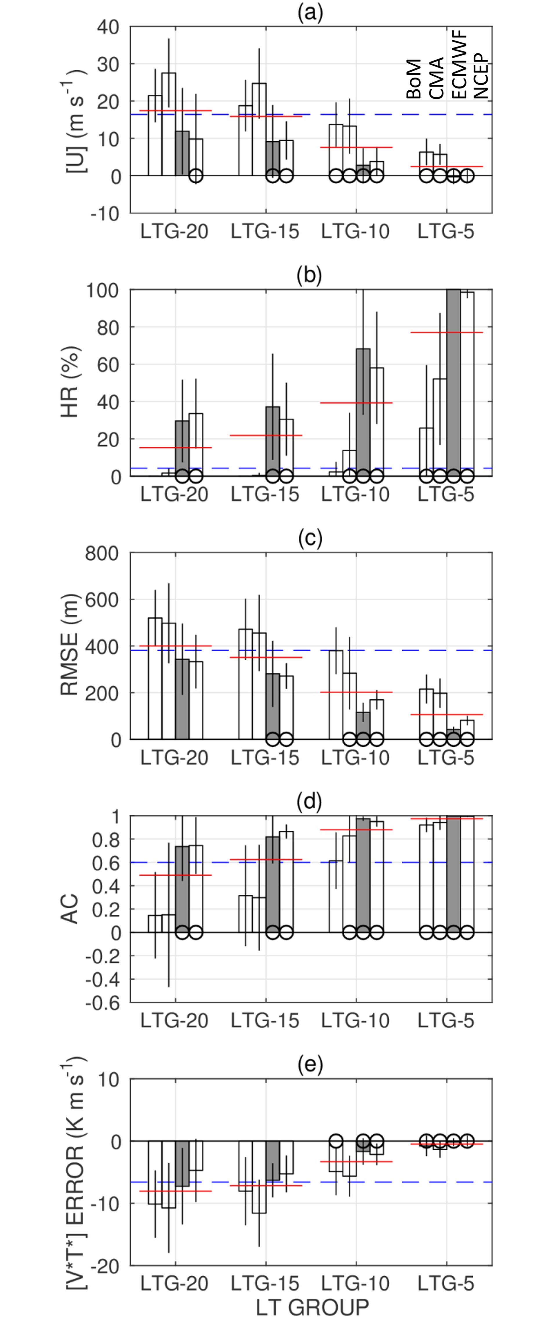Figure5. Variations in the five forecast verification measures with the four LTGs and four systems: (a) [U] (units: m s^?1); (b) HR (units: %); (c) RMSE (units: m); (d) AC; and (e) waves 1–3 [V*T*] error [units: K m s^-1], as defined in section 2.2. The results for each LTG are plotted as the mean ± one standard deviation across the MSSWs #10–#21 for each system (#11–#20 for NCEP). Filled bars are for ECMWF. Red lines take the means across the four systems. Blue broken lines denote reference values (see section 3). Each circle indicates that the verification result is judged better than the reference value by a Student’s t-test at the 90% level (one-sided test).


The figure also includes reference values (blue broken lines) obtained from the JRA-55 data to be compared with the verification results. The reference values in Figs. 5a, c and e are based on the standard deviation of the respective quantities during DJF. For example, in Fig. 5a, anomalies of [U] (5 d running mean) from its climatology are used, and the standard deviation of all daily anomaly data for DJF is obtained. The reference value in Fig. 5b is the climatological occurrence frequency of MSSWs (0.043 events per 7 d): 22 MSSWs occur for DJF (regarded as 90 d) of 40 yr (the value is further multiplied by seven, because the ±3 d time difference is allowed for HR). Figure 5d uses a constant value of 0.6 as a reference.
A comparison of the verification results to the reference values suggests that the forecast verifications for LTG-10 and LTG-5, when averaged among the systems (red lines), are clearly better than the references. The LTG-10 and LTG-5 results for each system are also better than the references for most cases. The multi-system mean verifications for LTG-20 and LTG-15 are close to the reference values, except for HR. One also notices that some systems, such as ECMWF and NCEP, yield more successful forecasts. Specifically, even some of the LTG-20 and LTG-15 forecasts of ECMWF and NCEP can be regarded as successful.
When the multi-system mean results are compared with the results from Taguchi (2016a) for the MSSWs #13–#21 using the JMA forecasts, it suggests that they are comparable. For example, the zonal wind bias in Taguchi (2016a) is approximately 10 and 20 m s^?1 for lead times of 10 and 20 d, respectively. These values are close to the results in Fig. 5a.

Next, the focus is on the possible differences in forecast verifications between VD and VS MSSWs. In addition to the average results across all MSSWs, Figs. 3e–l also show composite [U] time series taken separately for the VD and VS MSSWs, when they are classified using the wave 2 amplitude (section 2 and Table 1). Inspection of the composite results suggests that the HC zonal wind, e.g., of LTG-15 and LTG-10, around the onset dates is generally stronger for the VS MSSWs than for the VD MSSWs; i.e., the HC data tend to underestimate the zonal wind deceleration to the MSSWs in the JRA-55 data more strongly for the VS MSSWs. This feature reflects that the deceleration to the MSSWs in JRA-55 is stronger for the VS MSSW, and such MSSWs of stronger deceleration will be more difficult to forecast, as shown by Rao et al. (2019a).
Such differences in the vortex strength in the HC data between the two MSSW types are also seen in the Z10 maps for LTG-15 (Figs. 4f–o). The differences between the HC data and the JRA-55 data are generally larger in magnitude for the VS MSSWs, consistent with the stronger underestimation in the zonal wind deceleration. The JRA-55 Z10 field shows a more elongated structure of the vortex for the VS MSSWs than for the VD counterpart. Such an elongated structure is basically absent from the HC data, as the HC Z10 patterns are more or less similar between the two types, with lower Z10 values for the VS MSSWs in places.
Figure 6 is a statistical summary example similar to Fig. 5, but compares composite verification results between the VD and VS MSSWs using the ECMWF HC data. The results show that the VS MSSWs of larger wave 2 amplitudes mostly have larger errors or lower skill for LTG-20, LTG-15 and LTG-10, regardless of the verification measures. Some of the differences are judged to be statistically significant at confidence levels higher than or around 90%, but others are not. The statistical significance was examined with the Student’s t-test (one-sided test hypothesizing larger forecast errors for the VS MSSWs). Such differences are less conspicuous for LTG-5.
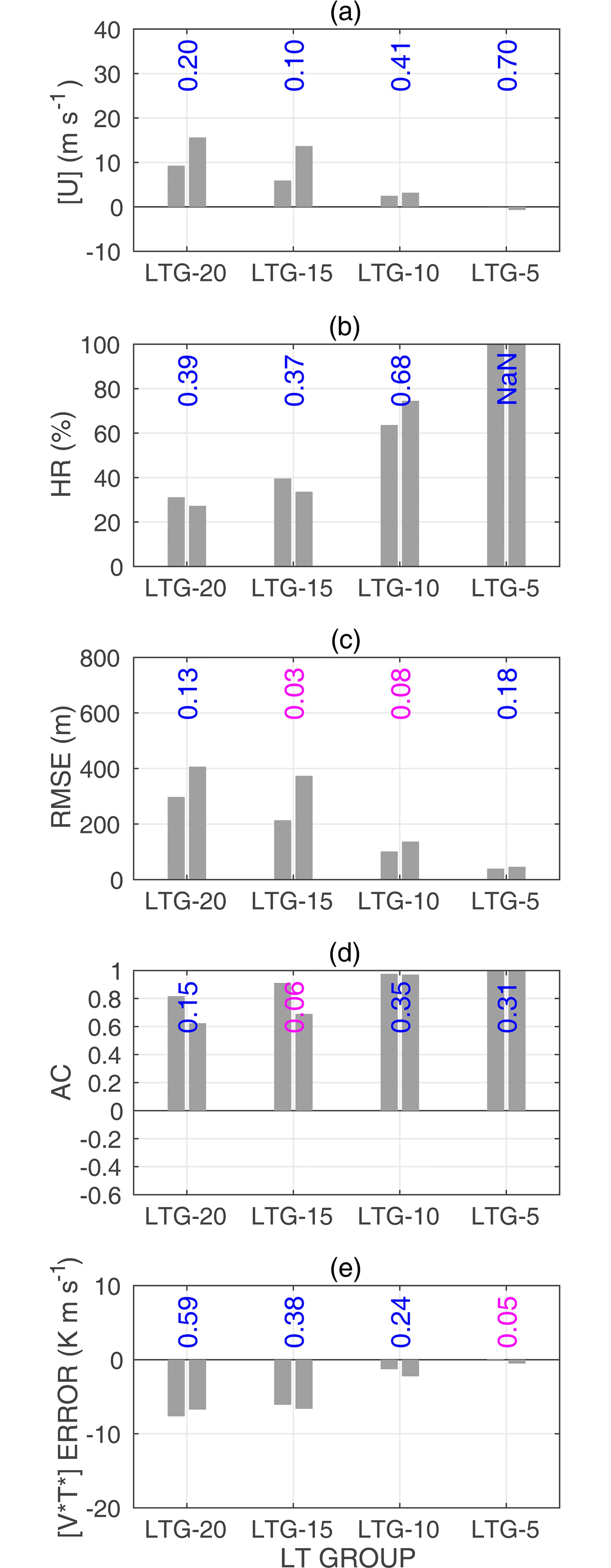Figure6. Bar chart showing composite results for VD MSSWs (left bar in each bar set) and VS MSSWs (right bar) for each LTG of the ECMWF HC data. The VD and VS MSSWs are classified using the wave 2 amplitude (Table 1). Panels (a–e) examine the same quantities as in Fig. 5. Each bar set shows the p value from the Student’s t-test (one-sided test hypothesizing larger errors or lower skill for the VS MSSWs). The numbers are denoted in magenta when smaller than 0.10.


This analysis was repeated for all systems and methods to classify the MSSWs, and the results are summarized in Fig. 7. The results support larger forecast errors or lower skill for the VS MSSWs in most cases (denoted by circles). The figure also plots the p values from the Student’s t-test hypothesizing larger forecast errors or lower skill for the VS MSSWs (color shading). The results are basically dominated by small p values (e.g., smaller than 20%, shown by warm colors), supporting the greater difficulty in forecasting the VS MSSWs, although statistical significance is not obtained for almost all cases. Note that the warm colors in Fig. 7 are applied using a relaxed threshold of 20%. This limitation is likely to reflect the limited sample size of the MSSWs at least partly, as this study uses 12 (or 10) MSSWs in contrast to 21 MSSWs in Taguchi (2016b). No strong dependence of the results on the verification measures or classification methods is seen.
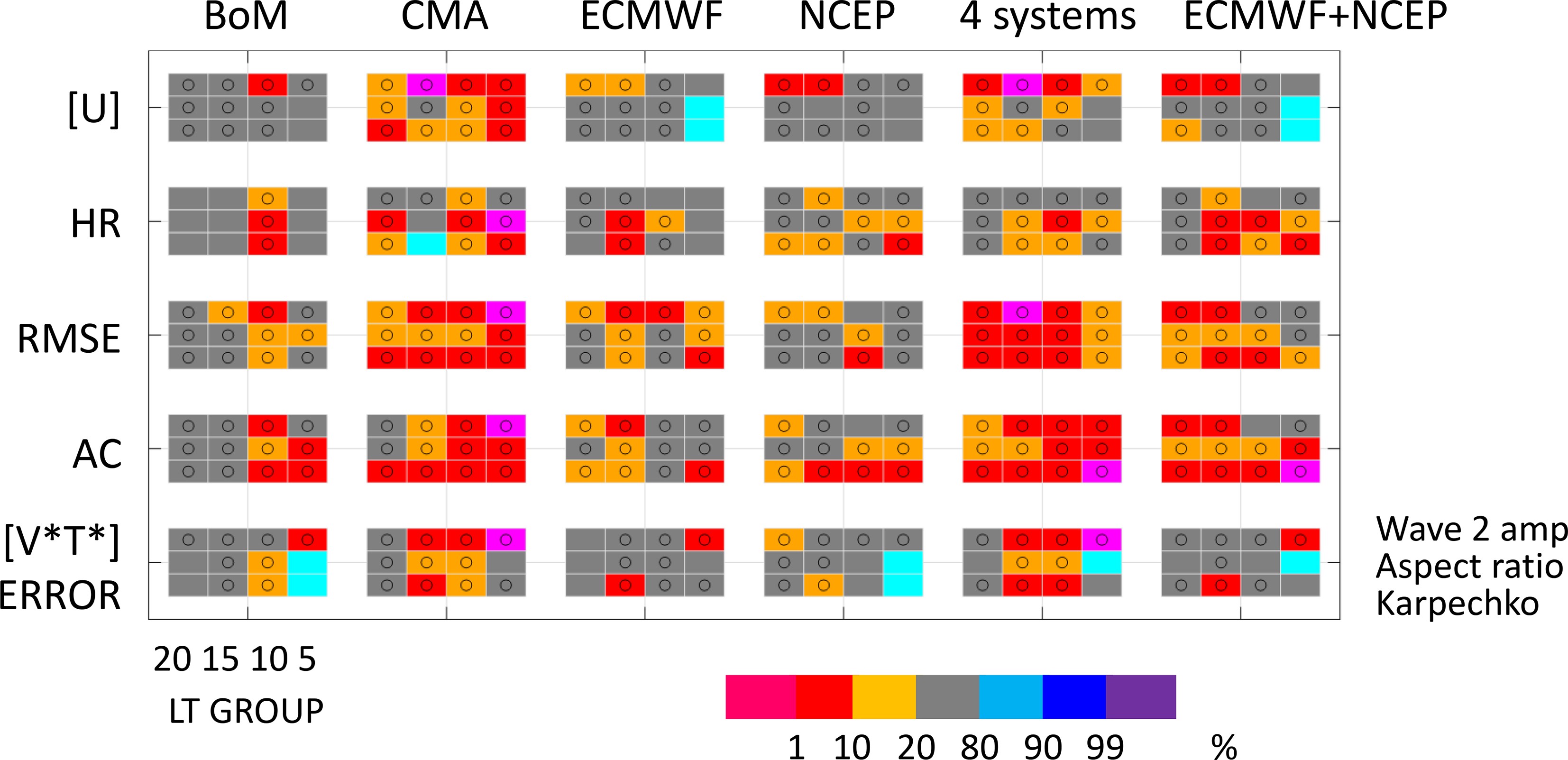Figure7. Student’s t-test results for the differences in forecast verifications between VD and VS MSSWs. Each circle denotes a larger forecast error or lower skill for VS MSSWs. Color shading denotes the p values of the test (one-sided test) when hypothesizing larger errors or lower skill for VS MSSWs (see the colorbar). The results are plotted for the different verification measures (rows) and systems (columns). Each set further consists of the different LTGs and methods to classify the MSSWs.


When comparing the different systems, the results from CMA support the differences most robustly. The results from CMA seem to dominate those combined from the four systems. The verifications for ECMWF and NCEP, which provide more successful forecasts (section 3), have statistical significance in more limited cases. Combining the ECMWF and NCEP results leads to increased cases of statistical significance, except for the heat flux errors.

This study has reported verification results of HC data from four S2S systems for MSSWs in northern winter from 1998/99 to 2012/13. The report deals with average features across all available MSSWs, and possible differences between VD and VS MSSWs.
Regarding the average features, results show that the stratospheric forecast verifications, when further averaged among the four systems, are judged to be successful for LTG-10 and LTG-5. All systems are skillful for LTG-5, whereas the results vary among the systems for longer lead times. Some systems (ECMWF and NCEP) are skillful for LTG-15 and LTG-20 in terms of the stratospheric measures, whereas others are not. These differences in the stratospheric forecast verifications among the lead times and systems correspond to those in the lower-stratospheric heat flux errors. The differences among the systems are consistent with Taguchi (2018) and Domeisen et al. (2019). The systems of the higher forecast skill have higher resolutions of the atmospheric models (Vitart et al., 2017), and future research could further explore possible relationships between them.
As for the possible differences between VD and VS MSSWs, our analysis overall suggests larger forecast errors or lower skill for the VS MSSWs, as argued by previous works (Taguchi, 2016b, c, 2018; Rao et al., 2018). The differences will be partly related to the fact that the VS MSSWs experience more rapid vortex weakenings (Rao et al., 2019a). However, these differences do not have statistical significance at high confidence levels for almost all cases, except for CMA. This limitation likely reflects the small sample size of the MSSWs analyzed in this study. Since this is constrained by the periods of the HC data, it would be desirable to examine this issue using more MSSW samples or longer HC periods.
The focus of this study on MSSW forecasts was partly motivated by the importance of MSSWs (extreme stratospheric states more generally) in tropospheric weather forecasts. The importance has been recognized in previous studies (see section 1), but a more direct demonstration of relationships of forecasts between MSSWs and anomalous weather conditions is relatively unpracticed. Such a demonstration, e.g., using the S2S database, is a possible future line of study.
Acknowledgements. The author thanks those who made the analyzed data available. The JRA-55 data used for this study were provided by the JMA. The JRA-55 data were obtained from the Research Data Archive at the National Center for Atmospheric Research, Computational and Information Systems Laboratory (https://doi.org/10.5065/D6HH6H41). The S2S data were obtained from the ECMWF server (http://apps.ecmwf.int/datasets/data/s2s/). This study was supported by JSPS KAKENHI (Grant No. JP17H01159), and discretionary expense of the President of Aichi University of Education. Comments from two anonymous reviewers improved the manuscript.