HTML
--> --> -->Seasonal forecasts were initially based on estimates of signal-to-noise ratios that assumed full knowledge of ocean and/or land conditions, such that the variance of climate variables related to lower boundary forcing represented the signal. However, it has been shown that the interaction between the atmosphere, sea ice, land and ocean are also important (Doblas-Reyes et al., 2013). Seasonal climate forecasting centers around the world now routinely run coupled ocean–atmosphere general circulation models (GCMs). GCMs parameterize physics on coarse grids but involve coupling of ocean and atmosphere modules. The main aim of GCMs is to produce intra- to interseasonal forecasts driven by the slowly evolving boundary conditions, such as sea surface temperature (SST) (Duan et al., 2019).
Ensemble forecasting is a technique used in numerical forecasts such that, instead of a single forecast, a series of forecasts depicting a wide range of future possible conditions in the atmosphere are produced. Nowadays, various centers produce ensemble forecasts of meteorological variables, such as precipitation and temperature, at different lead times from hourly to yearly, on a global scale, using numerical solutions of atmospheric hydrodynamic equations based on different initial conditions. Such forecasts have offered new opportunities in the water management sector. The Copernicus Climate Change Service (C3S) database has recently released the products of several significant European centers.
The C3S database combines weather system observations and provides comprehensive information on the past, present and future weather conditions. The service, run by ECMWF on behalf of the European Union, provides seasonal forecasting protocols on its website. The C3S Seasonal Service is publicly available through the Climate Data Store. Since the C3S database has been only recently launched, not much research on its evaluation has been reported. Forecast skill assessment can provide valuable information for forecasters and developers such that decision makers may adopt appropriate strategies to mitigate climate-related risks.
Manzanas et al. (2019) bias-corrected and calibrated C3S ensemble seasonal forecasts for Europe and Southeast Asia. The study adopted the ECMWF-SEAS5, UKMO-GloSea5 and Meteo France System5 models with a one-month lead time. For post-processing, simple bias adjustment (BA) and more sophisticated ensemble recalibration (RC) methods were employed, with the RC methods improving the reliability and outperforming the BA methods. The seasonal precipitation forecasts at the global scale were evaluated by Manzanas et al. (2014), who concluded that the best predictive skills were obtained in September–October and the poorest in March–May. MacLachlan et al. (2015) found that UKMO-GloSea5 had great forecast skill and reliability in predicting the North Atlantic Oscillation and Arctic Oscillation. Li and Robertson (2015) evaluated the ensemble forecast skill of the ECMWF, Japan Meteorological Agency (JMA) and CFSv2 models (seasonal center model of the NCEP) for summer and up to a four-week lead time. All three models provided good results for the first-week lead time. The forecast skill significantly declined in most clusters (except in some tropical clusters) during the second to fourth weeks. The precipitation forecast skill of the ECMWF model was significantly better than those of the other two models, especially for the third and fourth weeks. Shirvani and Landman (2016) studied the seasonal precipitation forecast skills of the North American Multi-Model Ensemble (NMME), two coupled ocean–atmosphere models and one two-tiered model, over Iran. They found low forecast skill for most models at all lead times, except in the October–December period at lead times of up to three months.
Crochemore et al. (2017) evaluated the seasonal forecast skill of precipitation and river flow in 16 watersheds in France. The hindcasts of the ECMWF seasonal precipitation model (System 4) with a 90-day lead time were evaluated and post-processed using SAFRAN data (Météo France reanalysis product). They employed linear scaling (LS) and monthly and annual distribution mapping to post-process the raw precipitation data. The results indicated an increase in precipitation forecast skill after applying post-processing methods. Bett et al. (2017) assessed the skill and reliability of wind speed in GloSea5 seasonal forecasts corresponding to winter and summer seasons over China. The results showed that the winter mean wind speed was skillfully forecasted along the coast of the South China Sea. Lucatero et al. (2018) examined the skill of raw and post-processed ensemble seasonal meteorological forecasts in Denmark. They took advantage of the LS and quantile mapping (QM) techniques to bias-correct ECMWF precipitation, temperature and evapotranspiration ensemble forecasts on a daily basis. The focus was on clusters where seasonal forecasting was difficult. They concluded that the LS and QM techniques were able to remove the mean bias. Regarding the estimation of dry days and low precipitation amounts, the efficiency of QM was better than that of LS. Mishra et al. (2019) provided one of the most comprehensive assessments of seasonal temperature and precipitation ensemble forecasts of the EUROSIP multi-model forecasting system. One equally and two unequally weighted multi-models were also constructed from individual models, for both climate variables, and their respective forecasts were also assessed. They found that the simple equally weighted multi-model system performed better than both unequally weighted multi-model combination systems. Zhang et al. (2019) evaluated the ability of the seasonal temperature forecasts of the NMME over west coast areas of the United States. In general, the skill of the one-month lead time NMME forecasts was superior or similar to persistence forecasts over many continental clusters, while the skill was generally stronger over the ocean than over the continent. However, the forecast skill along most west coast clusters was markedly lower than in the adjacent ocean and interior, especially during the warm seasons.
To the best of our knowledge, no research has yet been reported in which the precipitation forecasts of the C3S database have been comprehensively evaluated. In this study, the ECMWF, MF (Météo France) and UKMO ensemble precipitation forecasts were extracted from the C3S database in Iran’s geographical area for a period of approximately 24 years (1993–2017). The forecasts were compared with station data in different precipitation clusters. Evaluation of raw forecasts was performed in two stages: deterministic and probabilistic assessment.
| Origin | Lead time | Resolution of model (horizontal/vertical) | Forecasts | Hindcasts | |||
| Ens. size and start dates | Production | Ens. size and start dates | Production | ||||
| ECMWF (SEAS5) | 1–7 months | Dynamics: TCO319 cubic octahedral grid; Physics: O320 Gaussian grid (36 km) / 91 levels in vertical, to 0.1 hPa (80 km) | 51 members start on the 1st | Real-time | 25 members start on the 1st | Fixed dataset | |
| UKMO (GloSea5) | 1–7 months | N216: 0.83° × 0.56° (approx. 60 km in midlatitudes) / 85 levels in vertical, to 85 km | 2 members start each day | Real-time | 7 members on the 1st, 7 members on the 9th, 7 members on the 17th, 7 members on the 25th | On-the-fly | |
| MétéoFrance (System5) | 1–7 months | TL255: 0.7° Gauss reduced grid / 91 levels in vertical, to above 0.2 hPa | 51 members: 26 start on the first Wednesday after the 19th; 25 start on the first Wednesday after the 12th | Real-time | 15 members start on the first Wednesday after the 19th | Fixed dataset | |
Table1. Details of the selected numerical forecast models.
In this study, the ECMWF, MF and UKMO monthly ensemble precipitation hindcasts of the C3S database in Iran’s geographical area (25°–40°N, 44°–64°E) at an approximate 25-km spatial resolution (0.25° × 0.25°) were extracted for a period of 24 years (1993–2017) at a three-month lead time with a monthly time step. Observed point data were extracted for 100 synoptic stations, operated by the Iranian Meteorological Organization, spread over eight different precipitation clusters as classified by Modarres (2006) based on the geography and climate using the Ward method. Figure 1 shows a map of Iran’s precipitation clusters, over which the locations of 100 stations used in this study are overlaid. Cluster G1 involves arid and semi-arid clusters of central and eastern Iran, subject to high coefficient of variation and low precipitation. Cluster G2, spread in three distinct clusters (as shown in Fig. 1), mostly encompasses highland margins of G1. Cluster G3 involves cold clusters in northwestern Iran, while cluster G4 represents warm and temperate clusters along the Persian Gulf northern coast. Cluster G5 involves areas over the western border along the Zagros Mountains. Cluster G6, enjoying high precipitation, represents areas along the coast of the Caspian Sea in northern Iran. Cluster G7 is similar to G5 but receives more precipitation and encompasses two distinct clusters. In addition, cluster G8 is similar to G6, but receives more precipitation. Table 2 lists the number of stations and characteristics of the precipitation clusters.
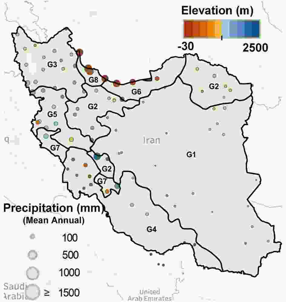 Figure1. Layout of the observation stations and G1–G8 precipitation clusters [the boundaries of the eight groups are based on the research of Modarres (2006)].
| Cluster | No. of stations | Area (km2) | Longitude (°E) | Latitude (°N) | Mean elevation (m) | Mean annual prec. (mm yr?1) | Characteristics |
| G1 | 27 | 847601 | 48.5–62.3 | 25.3–36.4 | 1238.7 | 186.23 | Arid and semi-arid clusters in central Iran |
| G2 | 20 | 192090 | 48.3–61.2 | 27.2–37.5 | 1064.3 | 246.68 | Highland margins of G1 |
| G3 | 19 | 128587 | 44.4–48.5 | 35.9–39.7 | 1368.9 | 350.39 | Northwestern cold cluster |
| G4 | 15 | 266031 | 48.0–57.8 | 25.6–32.3 | 368.5 | 265.36 | Coast of the Persian Gulf |
| G5 | 6 | 79172 | 45.9–47.2 | 33.6–35.3 | 1231.8 | 235.03 | Zagros Mountains cluster |
| G6 | 6 | 57230 | 49.8–54.4 | 34.1–36.9 | 685.2 | 803.25 | Lowland margins of the Caspian Sea |
| G7 | 3 | 36420 | 49.2–49.7 | 30.6–30.8 | 22.7 | 425.35 | Zagros Mountains cluster (precipitation in G7 is higher than G5) |
| G8 | 3 | 15299 | 48.9–49.6 | 37.3–38.4 | ?17.8 | 1472.26 | Lowland margins of the Caspian Sea (precipitation in G8 is higher than G6) |
Table2. Details of the precipitation clusters and the number of selected stations in each cluster (Kolachian and Saghafian, 2019).
Using the inverse distance weighting method (Ozelkan et al., 2015), the forecast data were interpolated to the selected stations, and then monthly precipitation forecasts were compared with observed data. Evaluation criteria were employed in two stages, including deterministic and probabilistic assessment. It should be noted that the averages of the evaluation criteria in each precipitation cluster are reported in this study. All the evaluation criteria formulae used in this study are presented in Table 3.
| Verification measure | Formula | Description | Perfect/no skill |
| Pearson’s correlation coefficient | $ r=\frac{\displaystyle\sum \left(F-\overline {F}\right)(O-\overline {O})}{\sqrt{\displaystyle\sum {(F-\overline {F})}^{2}}\sqrt{\displaystyle\sum {(O-\overline {O})}^{2}}} $ | Linear dependency between forecast and observation | 1/0 |
| Root-mean-square error | $ {\rm{RMSE}}=\sqrt{\dfrac{1}{N}\displaystyle\sum {\left[(F-\overline {F})-(O-\overline {O})\right]}^{2}} $ | Closeness between anomaly forecast and anomaly observation | 0 |
| Root-mean-square error skill score | $ {{\rm{RMSE}}}_{{\rm{S}}{\rm{S}}}=1-\dfrac{{\rm{RMSE}}}{{{\rm{RMSE}}}_{\rm{ref}}} $ | To understand values of RMSE | 1 |
| Relative root-mean-square error skill score | $ {\rm{R}}{\rm{RMSE}}=\dfrac{{\rm{RMSE}}}{\overline {O}} $ | To understand values of RMSE | 0 |
| Continuously ranked probability score | $ {\rm{C}}{\rm{R}}{\rm{P}}{\rm{S}}=\int {\left[{P}_{{\rm{F}}}\left(x\right)-{P}_{{\rm{O}}}\left(x\right)\right]}^{2}{\rm{d}}x $ | How well did the probability forecast the category into which the observation fell? | 0/1 |
| CRPS skill score | $ {\rm{C}}{\rm{R}}{\rm{P}}{\rm{S}}{\rm{s}}{\rm{s}}=1-\dfrac{{\rm{C}}{\rm{R}}{\rm{P}}{\rm{S}}}{{{\rm{C}}{\rm{R}}{\rm{P}}{\rm{S}}}_{\rm{ref}}} $ | Accuracy of the Probabilistic Quantitative Precipitation Forecasts (PQPFs) compared to the climatology | 1/$ \leqslant 0 $ |
| Relative operating characteristic skill score | ROCSS = 2A ? 1, A is the area under the ROC curve | Accuracy of PQPFs the in forecasting the occurrence or non-occurrence of events | 1/$ \leqslant 0 $ |
| Notes: F, O, PF and PO denote the forecast, corresponding observation, probability of precipitation and observed frequency, respectively; N is the amount of forecast and observation pairs. Similarly,$ \overline {F} $ and $ \overline {O} $ denote the forecast average and observation average. $ {{\rm{C}}{\rm{R}}{\rm{P}}{\rm{S}}}_{\rm{ref}} $ is the CRPS of the reference probability forecast, typically calculated from the climatology. 1 for perfect skill and 0 for no skill. | |||
Table3. Evaluation criteria used in this study (Tao et al., 2014; Aminyavari et al., 2018).
2
2.1. Evaluation criteria
For deterministic evaluation, the Pearson correlation coefficients were used to compare the forecast values with those of the observed. The root-mean-square error skill score (RMSESS) was also adopted, to calculate the error intensity of the forecasted monthly precipitation. Since each cluster has different mean precipitation, the skill score of this criterion was used for a fair assessment. The RMSESS is 1 for a perfect forecast, and 0 when the forecast equals the climatology. It should be noted that in order to prevent dispersion, anomaly forecasts and observations were used for calculating the RMSE. A monthly anomaly is the actual monthly value minus the climatology of the same month (i.e., the average over 1993–2017).For the probabilistic evaluation, the continuously ranked probability score (CRPS) and the relative operating characteristic (ROC) were used. To calculate the ROC, for each category (low/middle/upper tercile) a binary observation (0: the category occurred, 1: the category was not observed) and a probabilistic (between 0 and 1) forecast were created. The latter is derived based on the number of members predicting the category, out of the total number of available members. Then, for each tercile category, based on the values of hit and false alarm rates that were obtained based on a probability threshold varying from 0 to 1, the ROC curve was drawn and the area under the curve was calculated. Finally, the ROC skill score (ROCSS) was computed as 2A ? 1, where A is the area under the ROC curve. The ROCSS range is ?1 to 1, where zero indicates no skill when compared to the climatological forecasts and 1 represents the perfect score (Manzanas et al., 2014). Moreover, using the CRPS, the agreement of the cumulative distribution function (CDF) forecasts with the observed CDF was studied. The perfect score for the CRPS criterion is 0. The CRPS criterion was calculated based on Ferro et al. (2008). As with the reason for using the RMSEss, the CRPS skill score (CRPSss) was used for a fair assessment between clusters. The CRPSss was determined based on the relationship presented in Table 3.
The evaluation results were interpreted on a monthly, three-month average, and annual basis. On the monthly basis, the performance of each model was individually investigated in all 12 months; whereas for the 3-month average, the average precipitation in all four seasons was determined. Then, forecasts were evaluated in three (lower, middle and upper) tercile categories.
2
2.2. Multi-model forecasts
Three selected models were combined to generate multi-model forecasts using the simple arithmetic mean (MMM), multivariate regression (MRMM), and bias-removed (BRMM) techniques. In the MMM, simply the mean of the three model forecasts was calculated in each time step.In the MRMM combination, a multivariate regression was developed to combine the forecasts of the three models based on the following relationship (Zhi et al., 2012):
where


In the BRMM approach, a multi-model was generated based on the following relationship (Zhi et al., 2012):
The correlation coefficient and relative root-mean-square error (RRMSE) were used to evaluate and compare the skills of individual forecast models with the constructed multi-models. These criteria were selected based on a similar study by Zhi et al. (2012). Since precipitation varies greatly among clusters, the RMSEs of each cluster were divided by the mean observed value of the same cluster to make a fair assessment. It should be noted that the evaluations in this part of the study were carried out separately for the four seasons.
2
2.3. Evaluation based on drought indices
The Standardized Precipitation Index (SPI) was also adopted, to evaluate the skill of the models to forecast dry/wet years. The SPI represents the number of standard deviations (SDs) that observed cumulative precipitation deviates from the climatological average (Guttman, 1999). To calculate the SPI, the gamma distribution was fitted to 30 years (1987–2017) of monthly precipitation series and then converted into the standard normal distribution. The mean SPI of the stations in each of the eight precipitation clusters were determined and intercompared. The SPEI package (Beguería and Vicente-Serrano, 2017) was employed to calculate the SPI in R software.Further, to study the effect of climatic signals on precipitation changes in the study period, the Oceanic Ni?o Index (ONI) was extracted (
Also, regarding the effect that ENSO may impose on the skill of different models, tercile plots (Nikulin et al., 2018) were used to examine the sensitivity of the skill to El Ni?o, La Ni?a, and neutral years. The tercile plots were drawn using the visualizeR package in R software (Frías et al., 2018).
 Figure2. Average monthly forecasted precipitation values of ECMWF, UKMO and MF, along with observed data, in precipitation clusters with a one-month lead time.
In the following, first, the total precipitation forecasted during the study period will be evaluated. Then, the seasonal precipitation is examined in different clusters and terciles, and the performance of the models in different months is also interpreted. Then, the skills of multiple models are compared with individual models, and finally, based on the drought index, the quality of forecasts is evaluated.
2
3.1. Evaluation of total forecasts
The Pearson correlation coefficient results in Fig. 3 show that ECMWF and UKMO performed best in the G5 and G7 clusters, with over 70% significant correlation with observations. But, the correlation coefficients of MF were below 0.5 in most precipitation clusters. In the G6 and G8 precipitation clusters, encompassing the north of Iran, all models had correlation coefficients of less than 0.5, which were lower than in other clusters. Moreover, the skill of the models decreased with an increase in lead time. Overall, based on this criterion, the ECMWF model was in better agreement with the observations compared with the other two models, although UKMO was slightly better than ECMWF for a three-month lead time. Moreover, the SD of the correlation coefficients of the stations in each cluster is shown to understand the degree of dispersion in the evaluation result. As seen in the figure, in most clusters the SD is low and models perform the same at most stations. Only in clusters 6 and 8 is the SD slightly higher, which also affects the evaluation results of these two clusters.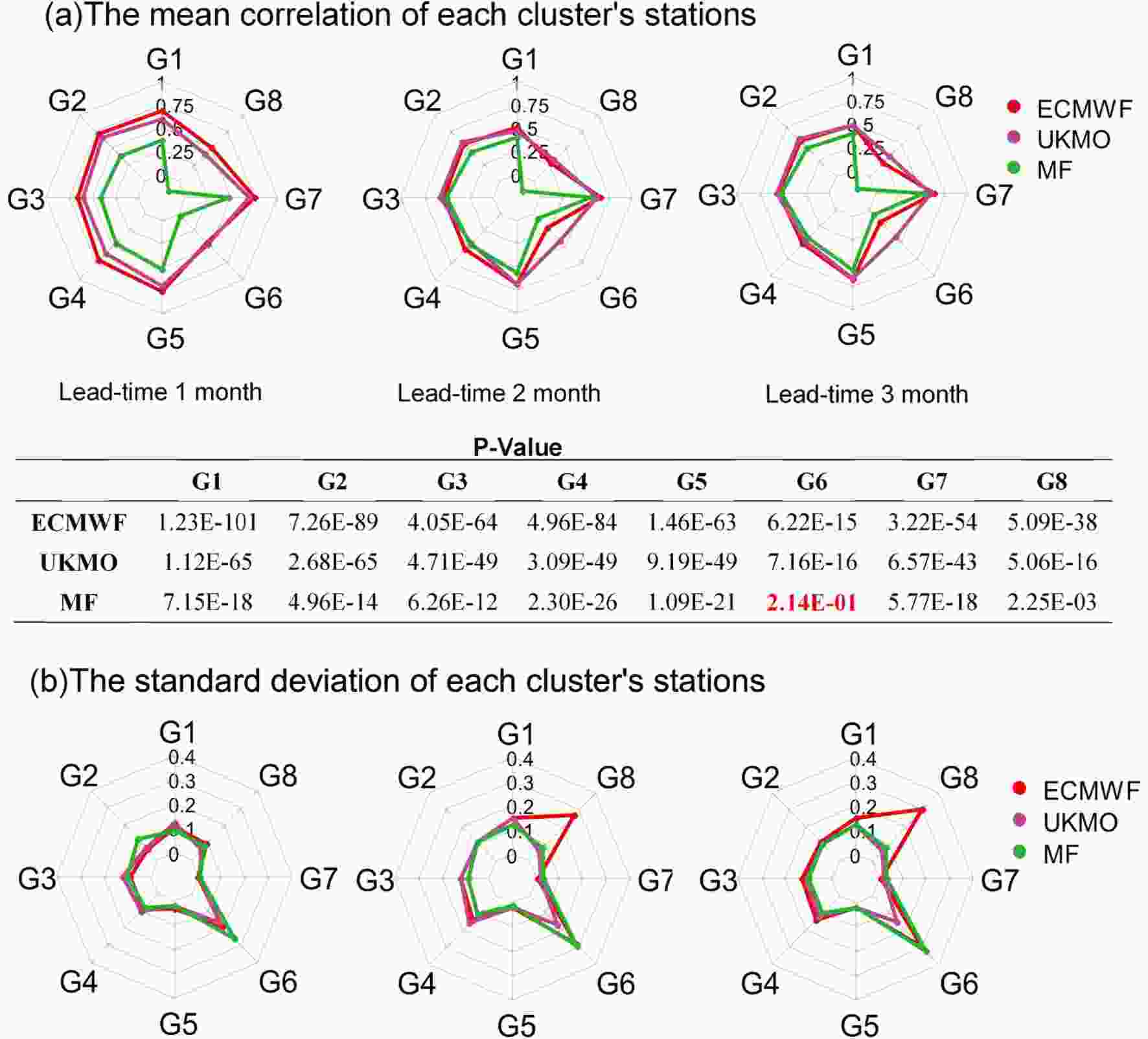 Figure3. Evaluation using the (a) mean and (b) SD of the Pearson correlation coefficient in each cluster. The table in panel (a) shows the P-values of the three models in the eight clusters (perfect score for the Pearson correlation coefficient is 1).
Pearson’s product-moment correlation statistical significance test was also performed, to determine whether the degree of correlation between models and observations was reliable. The P-values of the significance test, as shown in the table within Fig. 3a, indicates that the P-value in all models and clusters is less than 0.05, implying statistical significance of the correlation between the forecast models and observations. Only for the MF model in G6 cluster is the P-value slightly greater than 0.05.
The evaluation results of the RMSE skill score in Fig. 4 indicate that the models were more skillful in western Iran. However, in G3, encompassing northwestern Iran, the ECMWF model had a negative skill score and performed poorly in comparison with the reference forecasts. Similarly, UKMO provided poor forecasts in G3. The model also produced poor forecasts for the high-precipitation G8 cluster.
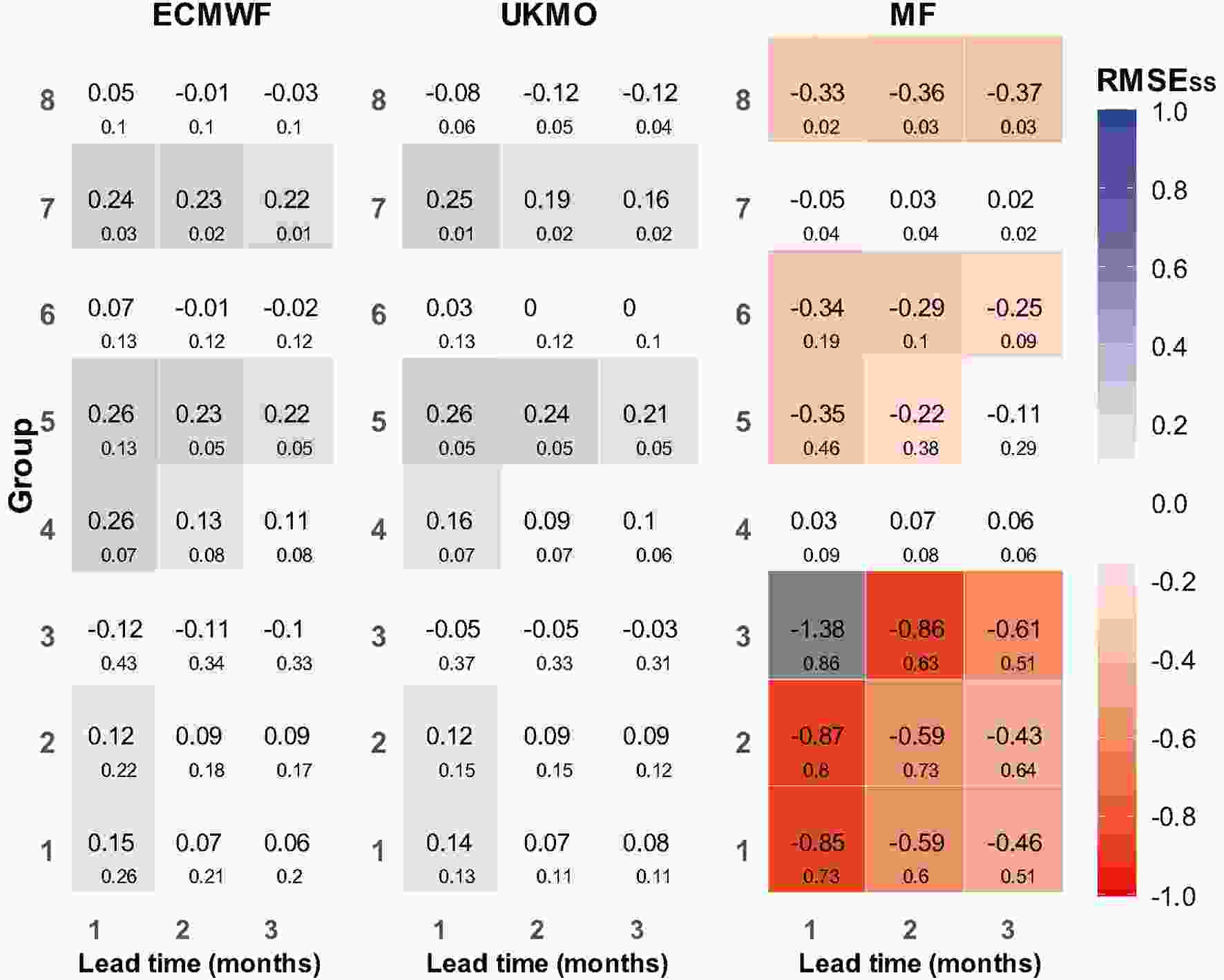 Figure4. Evaluation using the RMSESS in eight precipitation clusters (RMSESS is 1 for “perfect” forecast and 0 for “forecast equals climatology”).
The CRPSss results in Fig. 5 demonstrate that, in G4, G5 and G7, the models had closer CDFs to those of the observations and performed quite well in the clusters located in western Iran.
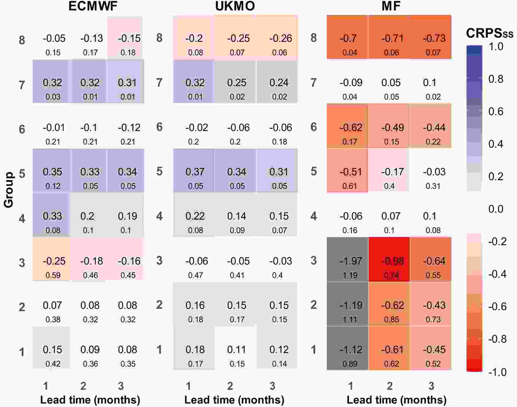 Figure5. Evaluation using CRPSSS in eight precipitation clusters (perfect score for CRPSSS is 1).
In general, the annual evaluation results indicated that the models provided better forecasts in western and southwestern Iran. In contrast, the models performed quite poorly in precipitation clusters in northern Iran. The ECMWF model outperformed the UKMO model in most evaluation criteria. The MF forecasts were poor. The gray cells in Figs. 4 and 5 are differentiated because their values are far from the other scores.
In Figs. 4, 5 and 7, the numbers in the squares correspond to the average score for the entire cluster (i.e., averaged over all stations within the cluster), while the small sized numbers indicate the SDs of the scores across all the stations in the cluster.
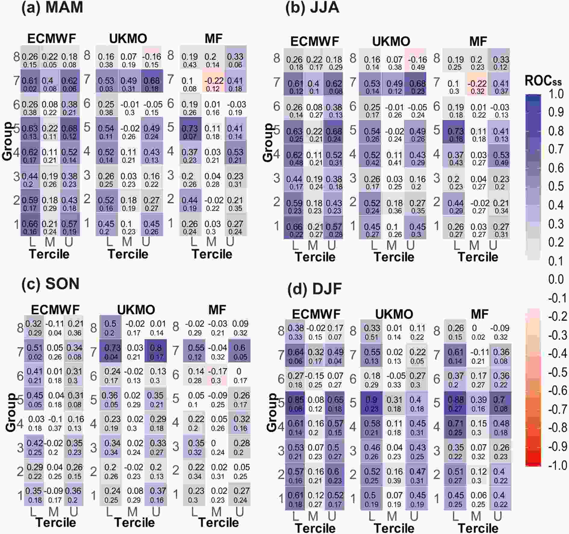 Figure7. Seasonal evaluation using ROCSS in eight precipitation clusters for three (L=lower, M=middle and U=upper) tercile categories (ROCss is 1 for “perfect” forecast and 0 for “forecast equals climatology”): (a) spring (MAM, March–April); (b) summer (JJA, June–August); (c) fall (SON, September–November); (d) winter (DJF, December–February).
Also, to understand why the forecasts were better in G1, G2, G4, G5 and G7, as compared with those in G3, G6 and G8, the time series of total annual precipitation is shown in Fig. 6. The results of the evaluation are fully consistent with Fig. 6, showing why the models have varying evaluation scores in different clusters.
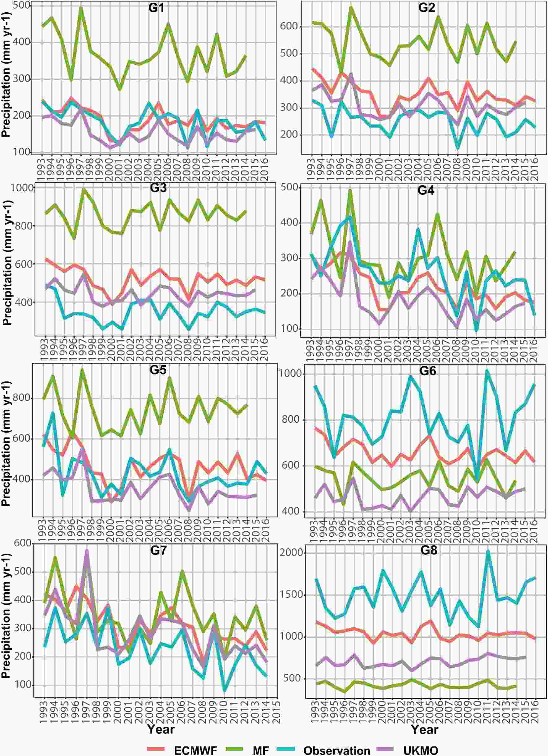 Figure6. Total annaul precipitation values of the ECMWF, UKMO and MF models, along with observed data, in precipitation clusters with a one-month lead time.
2
3.2. Evaluation of three-month average precipitation
In this section, the evaluation scores are reported based on three-month average observations and hindcasts at a one-month lead time. Based on Fig. 7, both the UKMO and ECMWF models yielded positive skill scores in most clusters (with the exception of northern climates in the G3, G6 and G8 clusters), indicating that the models forecasted the probability of occurrence better than the climatology. All three models had better proficiency scores in higher and lower terciles than in the middle tercile. In the summer, according to Fig. 7, the performance of all models declined compared to those in other seasons, whereas only the UKMO model scored higher in the G7 cluster.For the fall season, the ECMWF model forecasted light precipitation better than heavy precipitation. In this season, the MF model yielded a more accurate detection and lower false alarm rate than in other seasons. Overall, similar to the findings of Manzanas et al. (2014), all models produced better forecasts in this season than in the other seasons. In the G5 and G7 precipitation clusters, all three models performed better compared to the other seasons and precipitation clusters. In a similar study by Shirvani and Landman (2016), the best performance was found in the fall season. In winter, the performance of models was similar to that in the spring season, but with lower skill scores.
2
3.3. Evaluation of monthly precipitation
In this section, the performance of the models was investigated on a monthly basis in eight precipitation clusters. According to the Pearson correlation coefficients shown in Fig. 8, it is clear that the correlation coefficient decreased with increasing lead time. There was also no specific dependence between the lead time and the month of the year. The models produced good forecasts in spring months in dry climates, and in December in wet climates at two- and three-month lead times.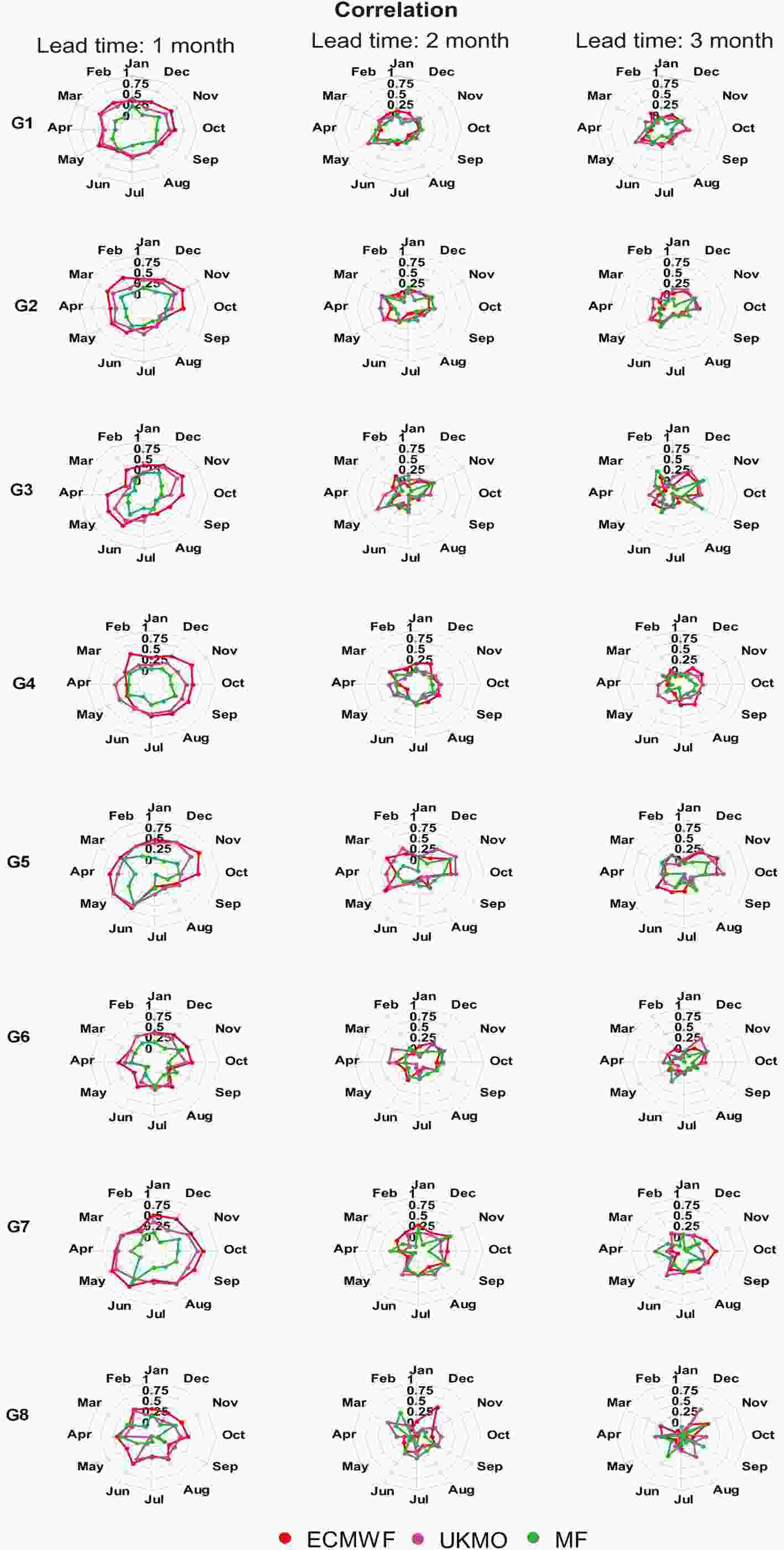 Figure8. Monthly evaluation using the Pearson correlation coefficients in eight precipitation clusters (perfect score for Pearson correlation is 1).
The ECMWF model performed best in November, while it had its poorest performance in August in most clusters. For western clusters in Iran, such as G7, which receive greater precipitation compared to central clusters, the model performed better in summer months than in other seasons; however, poorer forecasts were achieved in February. As mentioned in section 3.1, ECMWF did not provide acceptable performance in northern clusters. The UKMO model was to a certain extent similar in its performance to the ECMWF model, except that it performed best in dry central clusters in the winter. The UKMO model performed quite poorly in northern clusters in May. The MF forecasts did not correlate well with the observations in all months. For most clusters, this model provided better forecasts in March and April.
Also, to better assess the forecasts in different months, scatterplots of monthly forecasts over the study period are provided in Fig. 9. Based on the results of this study, the models had their best forecasts in G7 but their weakest ones in the G8 precipitation cluster. For the sake of brevity, scatterplots of only these two clusters are presented. According to Fig. 9a, in G7, observed precipitation was zero in the summer months, while the highest correlation occurred in January between the observations and ECMWF forecasts. From June to September, observed precipitation in this cluster was close to zero, so the highest ROCSS in section 3.2 was obtained in this period. This highlights that the ROCSS is conditioned on the observation such that the models accurately forecast dry conditions over that cluster. Also, in rainy months, the ECMWF and UKMO models performed well, and the scores shown in Fig. 9 may be attributable to the forecast skill.
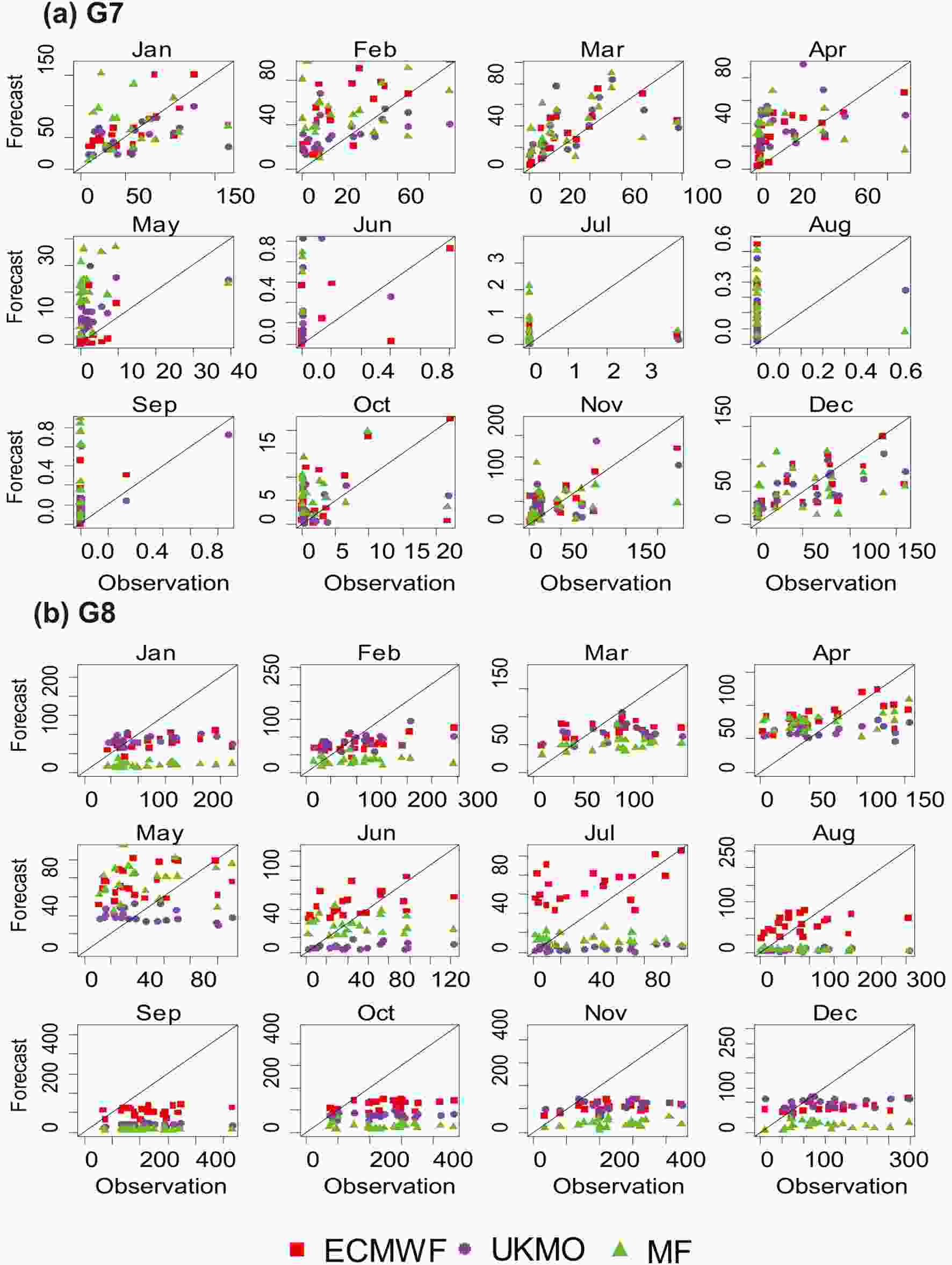 Figure9. Scatterplots of monthly precipitation in two precipitation clusters: (a) G7; (b) G8.
In the G8 precipitation cluster, most models underestimated the observations, with only the ECMWF model overestimating precipitation in the summer months. Although more precipitation occurred in winter than in spring, all models forecasted similar precipitation in these two seasons. All three models underestimated the fall and winter precipitation. The ECMWF model was a better performer than the other models.
2
3.4. Evaluation of multi-models
According to Fig. 10a, multi-models, especially MRMM, were better correlated with observations in most seasons and clusters than individual models, although MRMM had weaker forecasts in summer. The MF model in winter, especially in rainier clusters, showed no correlation with observations. Overall, the best forecasts for the multi- and individual models occurred in fall.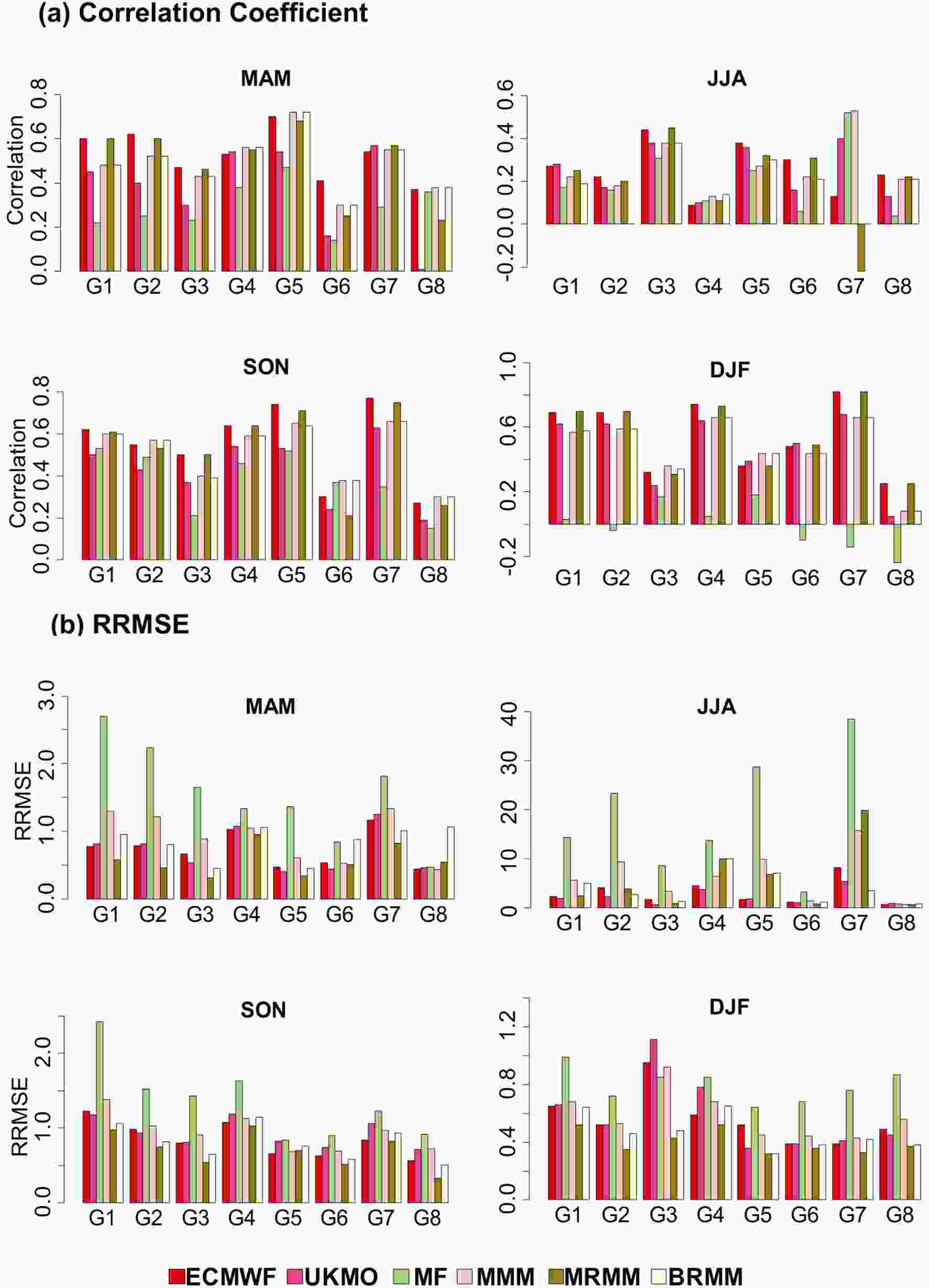 Figure10. Individual and multi-model seasonal evaluation using the Pearson correlation coefficient and RRMSE in eight precipitation clusters (perfect score for Pearson correlation is 1, and for RRMSE it is 1). MAM, March–May (spring); JJA, June–August (summer); SON, September–November (fall); DJF, December–February (winter).
Figure 10b shows the evaluation results of multi- and individual models using the RRMSE criterion. Of note is a large error in the MF forecasts. Despite the poor performance of the MF model, the three multi-models tended to provide similar results to those of the ECWMF and UKMO models, which represent the two best-performing individual models. Note that among the three multi-models, the MRMM provided the best overall results. The MRMM results showed that the model combination based on regression had a positive effect on reducing the forecast error of individual models. In accordance with previous studies (Doblas-Reyes et al., 2009; Bundel et al., 2011; Ma et al., 2012; Manzanas et al., 2014), the overall results in this section indicate that multi-models are effective in improving the predictive skill of individual models.
2
3.5. Evaluation of forecasted SPI
Figure 11 shows the time series of observed SPI and those corresponding to the ECMWF and UKMO model forecasts in eight precipitation clusters. The MF-derived SPI values are not shown here because of its poor performance. El Ni?o, neutral and La Ni?a years were extracted during the study period and added to Fig. 11. To better understand the performance of models in forecasting dry and wet years, the correlation coefficient between the SPI of the models and that of the observation is shown in Fig. 11. In G1, both models forecasted the wet years during 1995–2002 well, albeit with a slight overestimation by the UKMO model. Furthermore, both models forecasted the observed 2000–2002 dry period, although they extended the drought until 2004. In this cluster, the models forecasted a severe wet year in 1996, but the year was neutral based on the ONI. This was also the case for the 2001 severe drought, which was a La Ni?a year based on the ONI. Overall, the two models performed quite well in this cluster. In G2, the results were similar but weaker to those of the G1 cluster, whereas the UKMO model had poorer forecasts than the ECMWF model.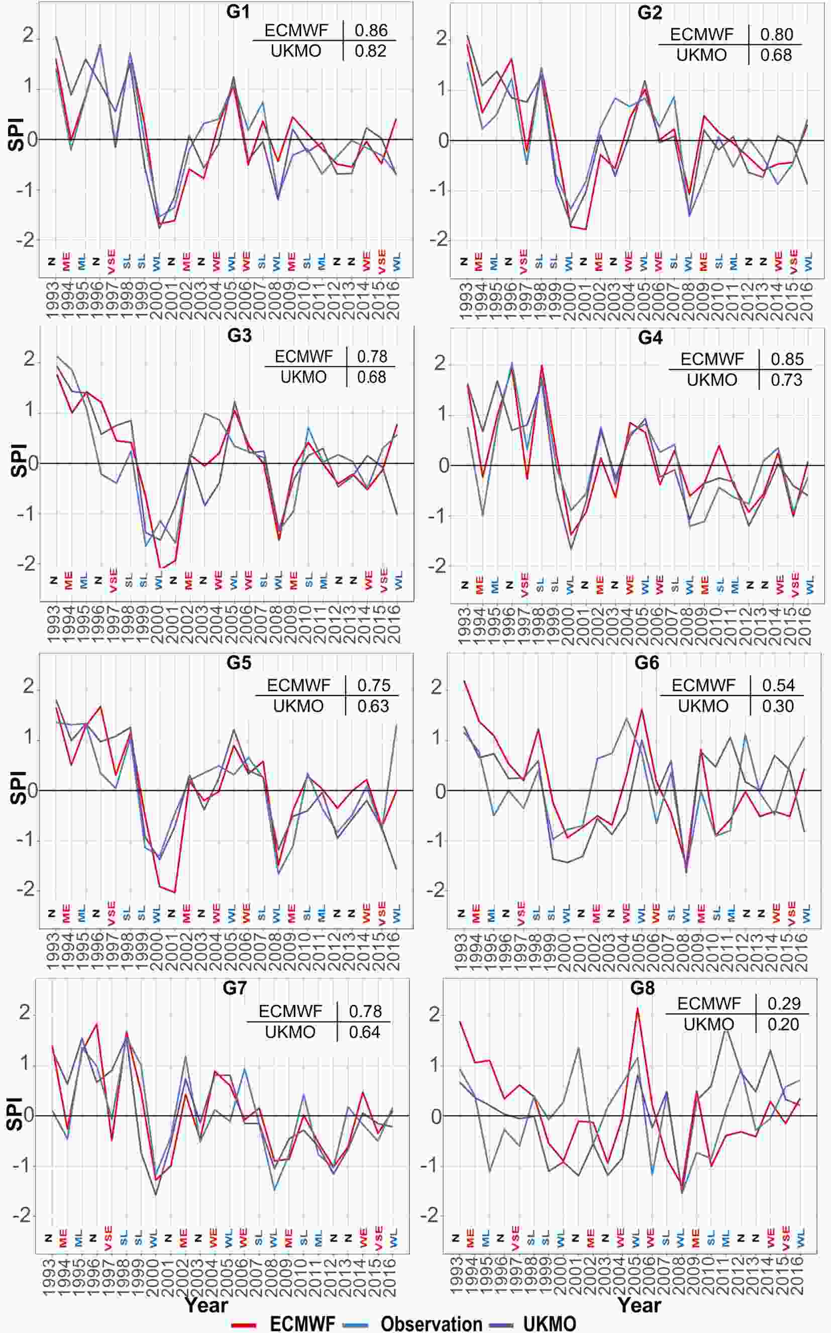 Figure11. Observed and forecasted SPI time series in G1 to G8 (the small 2 × 2 tables shown in the top-right corner of each panel indicate the correlation between the model-forecasted SPI and those of observations. N, neutral; W, weak; M, medium; S, strong; VS, very strong; E, El Ni?o; L, La Ni?a.
In G3, the UKMO model forecasted the severity of the SPI in wet and dry periods better than the ECMWF model. It should be noted that, while 1994 and 2008 were severe wet and drought years in the G3 precipitation cluster, respectively, El Ni?o and La Ni?a prevailed in 1994 and 2008. Thus, climate indices are not a good sign of wet/dry conditions in G3 in such years. In G4, ECMWF forecasted the drought/wetness index better than the UKMO model, although both models underestimated the dry periods in 2008–2012. Considering G5, ECMWF overestimated the drought from 2000 to 2003, while both models failed to forecast the wet year in 2016. In G6, the UKMO model slightly overestimated the dry periods. Both models forecasted the wet years from 1993 to 2000. However, the forecasted duration and intensity of wet years were shorter and weaker, respectively, than those observed.
Regarding G7, both models performed well and ECMWF forecasted the wet and dry periods quite close to the observations. Finally, in G8, both models had average performances and failed to forecast dry and wet periods. Overall, the models performed well in forecasting dry/wet periods in most clusters and, nearly in all clusters, they were able to detect the reduction in precipitation over the 2000–2001 period.
In examining the effects of ENSO in the study period, only heavy precipitation in 1995 could be marginally attributed to this phenomenon. Based on the work of Shirvani and Landman (2016), although ENSO is the main factor in seasonal forecast skill (Manzanas et al., 2014), no clearly strong predictive capability was found in this study for Iran. This may be partly attributable to the complicated precipitation variability in relation to SST patterns.
Finally, tercile plots were used to evaluate the impact of ENSO on the performance of models. For the sake of brevity, only the results of the G5 cluster, which had the best forecast results based on Fig. 7, are shown. According to Fig. 12a, although no clear relationship could be found between model performance and ENSO conditions, the ECMWF members of the ensemble forecast in El Ni?o years were slightly better than those in La Ni?a and neutral years. Moreover, according to Fig. 12b, the UKMO model did slightly better in the La Ni?a years. All in all, there is no clear connection between ENSO phenomena and precipitation predictability at seasonal time scales in Iran.
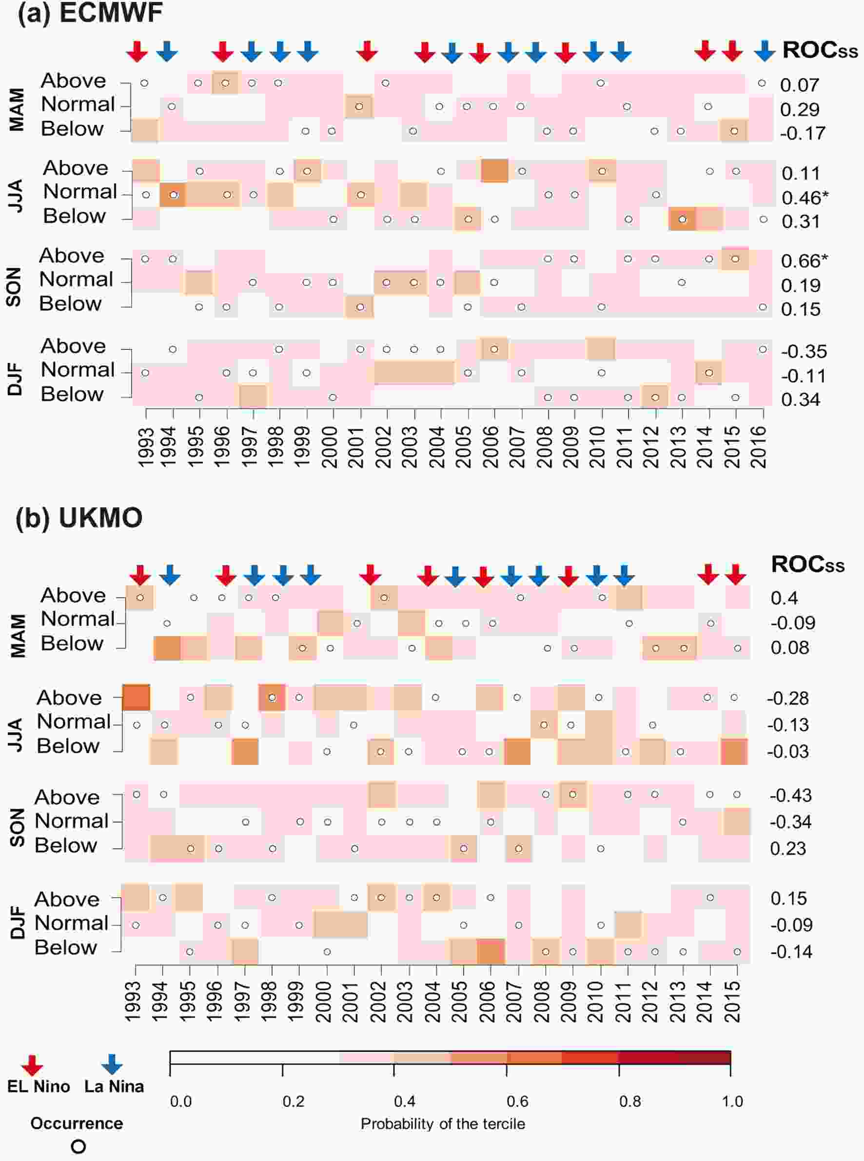 Figure12. Tercile plots for the (a) ECMWF and (b) UKMO models in the G5 cluster. The red color spectrum of each square represents the probability for each category (below, normal, above). Dots show the corresponding observed category for each year of the hindcast period. Numbers on the right show the ROCSS for each model and each tercile. (ROCSS is 1 for “perfect” forecast and 0 for “forecast equals climatology”).
(1) Based on the deterministic evaluation of the forecasts, the best correlation coefficients were achieved in the G5 and G7 clusters in western Iran, while the poorest performance was associated with G6 and G8 in northern Iran. Moreover, in forecasting the precipitation amount, all three models had their greatest error in G3 in northwestern Iran. The models performed well in the dry central and eastern clusters. The MF model had the greatest error among the models based on deterministic evaluation (Figs. 3 and 4).
(2) All models better forecasted upper-tercile events in dry seasons and lower-tercile events in wet seasons, but gained their lowest skill score in the middle category (Fig. 7) (similar to Manzanas et al., 2014, 2018).
(3) Based on probabilistic evaluation, all three models scored higher in the G5 and G7 precipitation clusters compared to those of other clusters (Fig. 5)
(4) In all evaluations, the skill of the models decreased with increasing lead time.
(5) In the monthly evaluation, the ECMWF model performed better in low-precipitation clusters in fall and in high-precipitation clusters in summer. On the contrary, the model performed poorly in northern clusters. The UKMO model yielded somewhat similar results, except the model performed better in low-precipitation clusters in the winter. In general, all three models overestimated precipitation in the summer (Fig. 8).
(6) The MRMM multi-model had better skill than individual models (Fig. 10).
(7) The forecast models had relatively good skill in forecasting dry and wet years, although they underestimated some dry years and overestimated some wet years (Fig. 11).
(8) No specific relationship was found regarding the influence of the ENSO climatic signal on model performance. The models did not yield acceptable forecasts in northern clusters where higher precipitation and relatively lower temperature prevail.
(9) In assessing the impact of climatic global signals on severe precipitation, the year 1995 may be considered to be significantly influenced by ONI phenomena, while no major effect was detected in other periods.
All in all, the evaluation results demonstrated that both the UKMO and ECMWF models perform well in forecasting monthly precipitation in Iran, especially in western precipitation clusters. However, it is not possible to clearly indicate which of the two models performs better. In most precipitation clusters at short lead times, the ECMWF model was better correlated with the observations and its forecasts gained higher skill scores. On the contrary, at a three-month lead time, the UKMO model had higher correlation coefficients with the observations in most precipitation clusters. The MF model is not an appropriate precipitation forecast model for Iran. Furthermore, the models are generally able to forecast dry/wet occurrences in Iran.
