HTML
--> --> -->Compared to other wind measurements, AMVs from geostationary satellites can provide superior temporal and spatial coverage in the middle and upper troposphere (Kaur et al., 2015), due to the capability of geostationary satellites in achieving frequent and continuous observations over a specific region (Honda et al., 2018). Various studies on the assimilation of AMVs derived from different satellites have been carried out to take advantage of such exceptional temporal and spatial overage, and positive results obtained. For example, AMVs from the Geostationary Operational Environment Satellite (GOES) have been assimilated in hurricane research, and the forecasts of hurricane tracks and intensity improved (Soden et al., 2001; Velden et al., 2017; Li et al., 2020). The assimilation of Kalpana-1 AMVs also reduced the initial position errors and improved track forecasts of tropical cyclones (Deb et al., 2011). Besides, studies on the assimilation of AMVs from MTSAT (Multi-function Transmission Satellite) and Himawari-8 showed positive impacts on the timing and intensity of rainfall forecasts, and even flood risk prediction (Yamashita, 2012; Otsuka et al., 2015; Kunii et al., 2016).
In addition to the satellites mentioned above, Fengyun (FY) geostationary satellites from China have also provided AMV products for operational NWP systems and the research community. Since the launch of the first Chinese geostationary meteorological satellite, FY-2A, in 1997, studies and applications of AMVs from Chinese geostationary meteorological satellites have been gradually increasing (Feng et al., 2008; Ren et al., 2014; Wan et al., 2018). Compared to the FY-2 series, the spatial and temporal resolutions have been dramatically improved in the FY-4A satellite, and two visible channels and seven infrared (IR) channels included. Moreover, it can produce full-disk imagery every 15 minutes, and the temporal resolution can be increased to up to 5 minutes for the coverage of China (Dong, 2016; Zhang et al., 2017; Wang and Shen, 2018; Zhao et al., 2019). The capability of obtaining AMVs has been greatly increased. However, studies on the AMV products of FY-4A are relatively rare (Wan et al., 2019). Therefore, in order to further understand the characteristics of FY-4A AMVs, and to promote the application of FY-4A AMVs in NWP, the characteristics of AMV products are analyzed in this study, and their impacts on data assimilation discussed.
The rest of this paper is organized as follows: Section 2 analyzes the characteristics of FY-4A AMVs, and the observation error of AMV products is estimated in section 3. Section 4 describes the framework of the assimilation and forecasting experiments, and results are discussed in section 5. Section 6 provides a summary of the study’s key findings.
2.1. AMV data from FY-4A
The monitoring and prediction of severe weather systems is one of the most important and complicated parts of operational weather forecasting. The Advanced Geosynchronous Radiation Imager (AGRI) onboard the FY-4A geostationary meteorological satellite plays a critical role in the monitoring of severe weather systems in China and its surrounding areas. There are 14 channels in AGRI, and AMV products used in this study are derived from channel 09 (λ = 6.5 μm), channel 10 (λ = 7.2 μm) and channel 12 (λ = 11.0 μm); namely, the high-level water vapor (WV-High) channel, the mid-level water vapor (WV-Mid) channel, and the IR channel, respectively. According to the documentation for FY-4A AMV products, the spatial resolution corresponding to the sub-satellite point is 64 km, and products with 3-h resolution can be provided. The horizontal distribution of FY-4A AMVs from WV-High, WV-Mid and IR at 0000 UTC 1 November 2018 are displayed in Figs. 1a-c. It is shown that the AMVs cover the West Pacific and Indian oceans, where conventional observations are sparse. Meanwhile, the horizontal distribution of AMVs from WV-High and WV-Mid are similar but different from that of IR. The IR channel supplements the AMV data of some regions where two water vapor channels are not observed. Figure 1d shows the calculation of the vertical profile of the total number of FY-4A AMVs for the three channels from 1?30 November 2018. The vertical distribution of AMVs derived from the two water vapor channels is obviously different from that from the IR channel, which is due to the difference in absorption characteristics of each channel. More specifically, WV-High and WV-Mid are in the water vapor absorption bands (Velden et al., 1997), and their different weighting function peak heights lead to the discrepancy in heights at which the channel AMV count is the most. In contrast, the IR channel is in the IR window band (Yang et al., 2014, Lu et al., 2017), so it can obtain AMVs of various heights, even data on the middle and lower troposphere.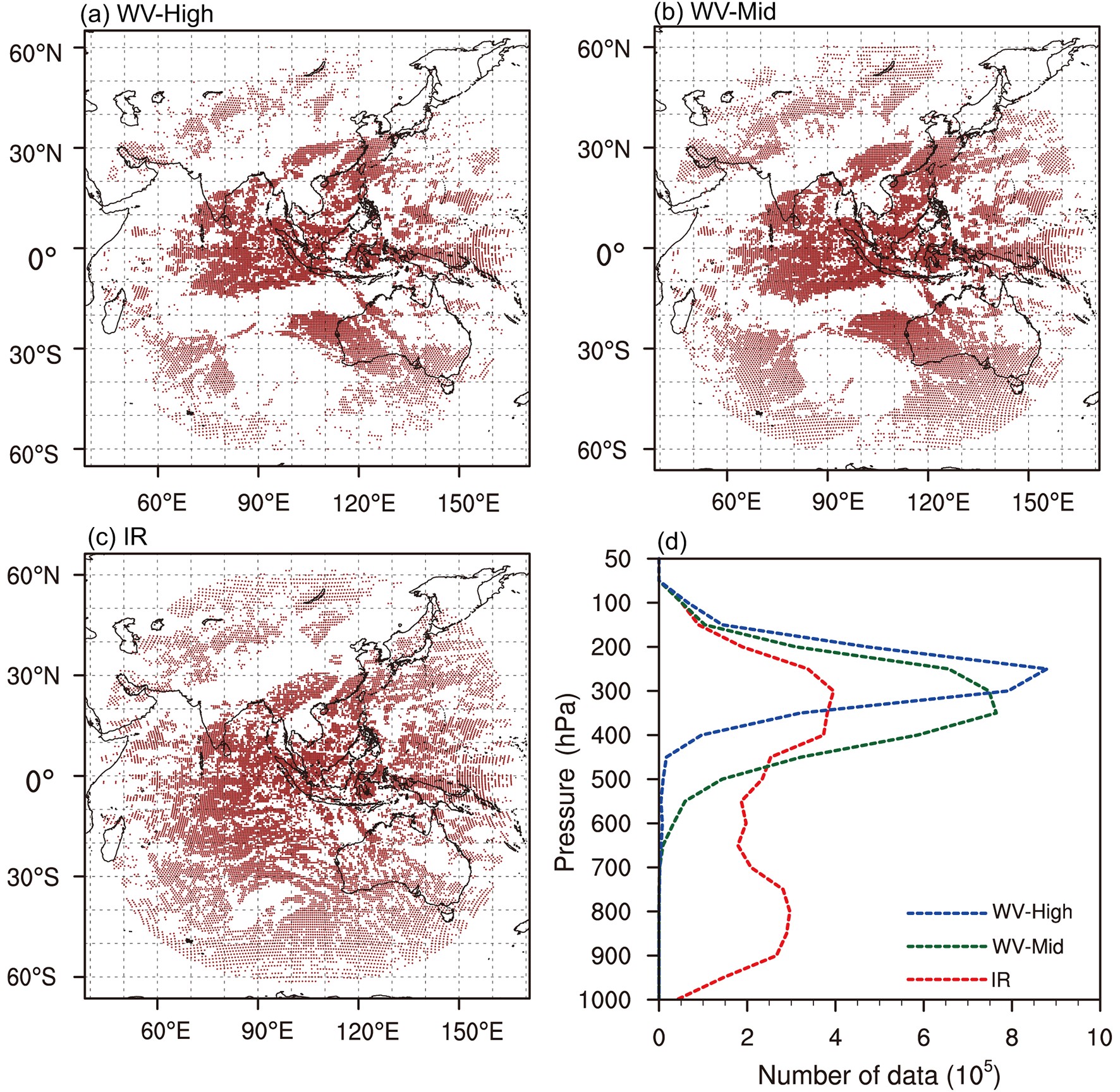 Figure1. Horizontal distributions of AMVs derived from (a) WV-High, (b) WV-Mid, and (c) IR at 0000 UTC 1 November 2018, and (d) vertical profiles of the total number of single AMV data from the three channels in each layer for the period from 1?30 November 2018.
2
2.2. Quality indicator for AMVs
The quality indicator (QI) is a weighted average of several normalized QI components, which is calculated to represent the quality of each FY-4A AMV (Holmlund, 1998). The QI value of FY-4A AMV is provided by the National Satellite Meteorological Center of China of the China Meteorological Administration (CMA). It is calculated as an empirical function of a spatial and temporal consistency check of wind speed, wind direction, vector and horizontal wind components. The value decreases as the agreement of a given vector with its surroundings decreases. As a result, a larger QI value means a higher credibility (Velden et al., 1998; Deb et al., 2015).Figure 2 shows the vertical distributions of FY-4A AMVs derived from the three channels from 1?30 November 2018 with different QI values. It can be seen that AMVs with different QI thresholds have similar vertical structure but the proportion of total amount is different. For example, AMVs with QI greater than 70 account for more than 80%, AMVs with QI greater than 80 make up about 60%, and AMVs with QI greater than 90 share only approximately 30% of the total data quantity.
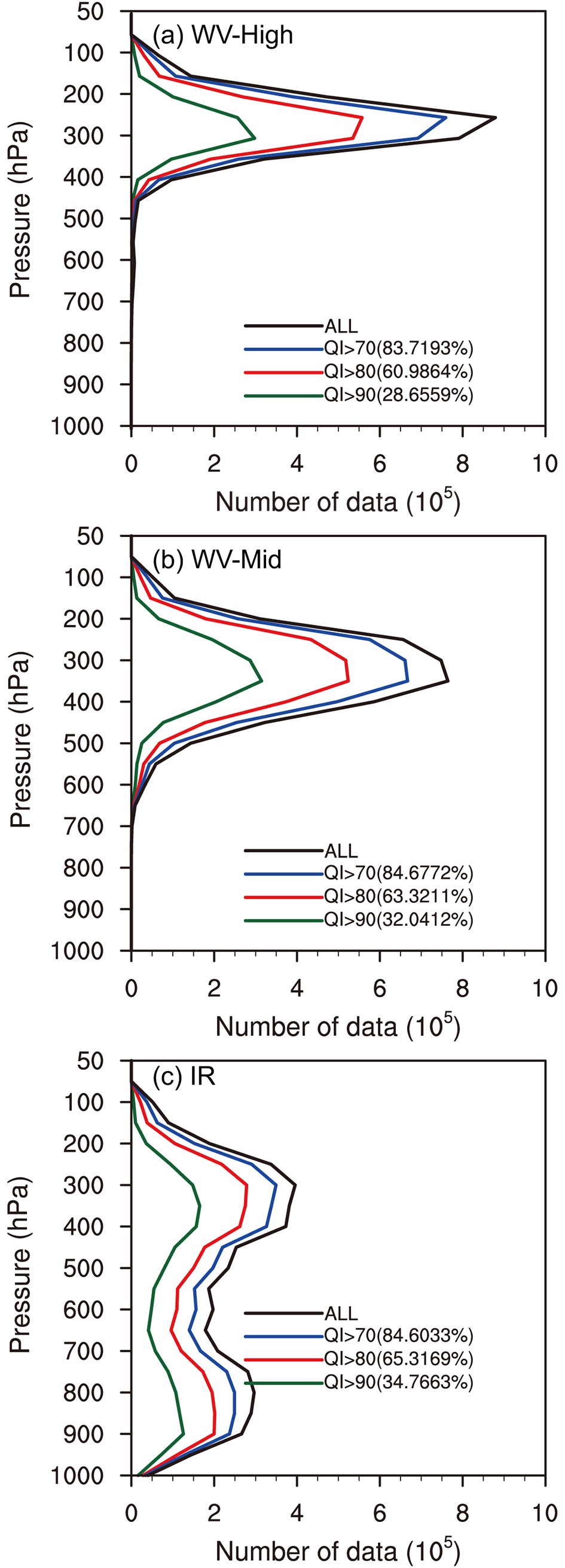 Figure2. Vertical distributions of AMVs derived from (a) WV-High, (b) WV-Mid, and (c) IR for the period from 1?30 November 2018 with different QI values (the values in brackets represent the percentage of the total amount of data under this threshold).
Next, the wind speed bias (Fig. 3) and root-mean-square error (RMSE) (Fig. 4) of FY-4A AMVs in November 2018 are calculated against the Final Operational Global Analysis (FNL) for FY-4A AMVs with different QI thresholds. As displayed in Fig. 3 and Fig. 4, smaller speed bias and RMSE of AMVs are obtained with a larger QI value, which is consistent with the conclusion obtained by Kim and Kim (2018). However, as the primary source of FY-4A AMVs below 500 hPa, data from the IR channel with QI greater than 80 (red line in Fig. 3c) have a slightly smaller wind speed bias than that with other thresholds, which is related to the AMV products themselves.
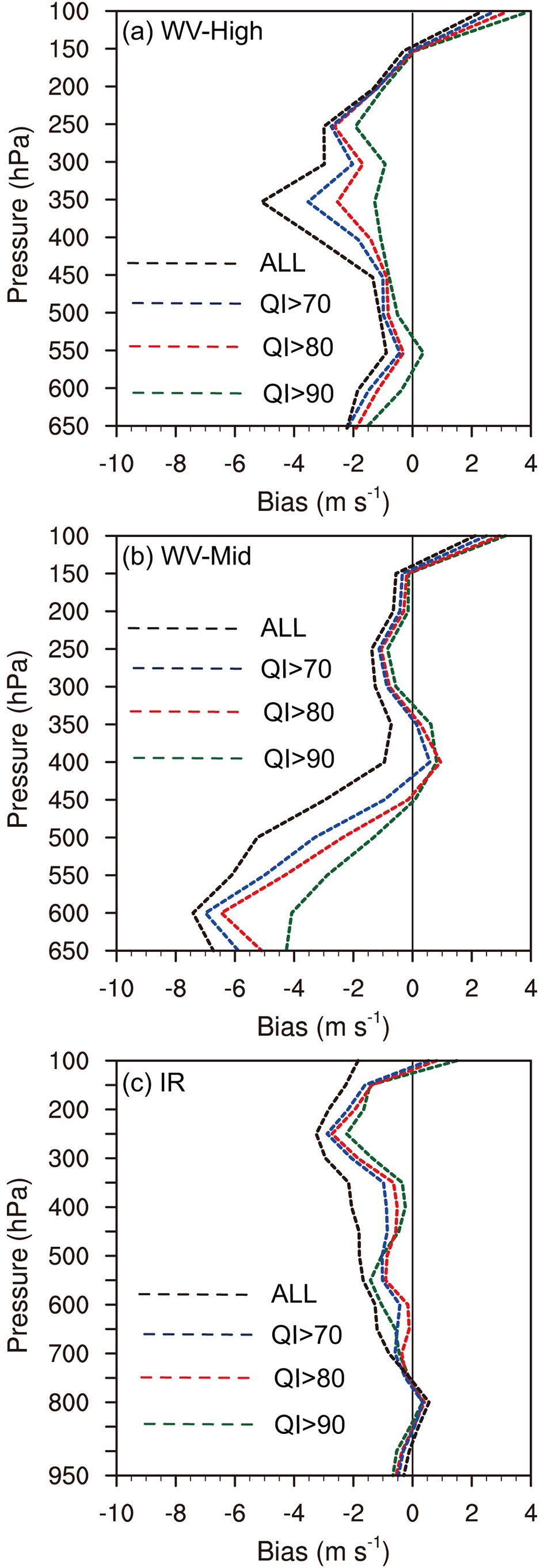 Figure3. Average wind speed bias against FNL AMVs derived from (a) WV-High, (b) WV-Mid, and (c) IR in November 2018 (the black solid line denotes that the bias of AMV data is zero).
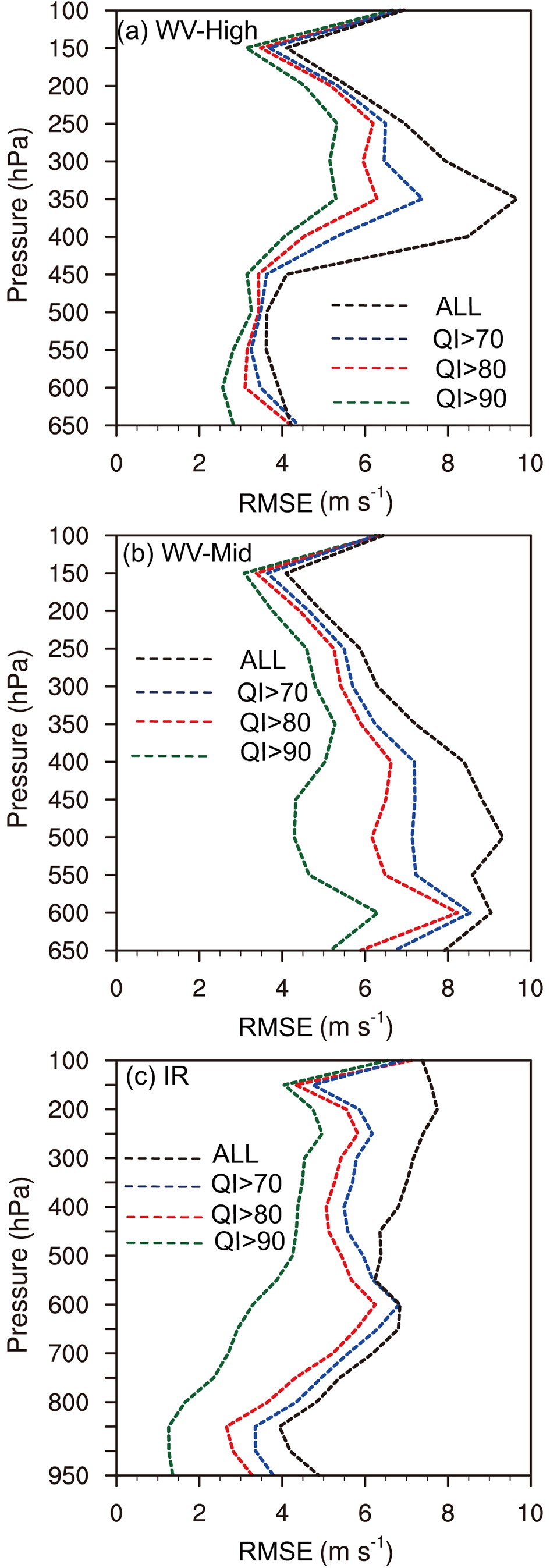 Figure4. Average wind speed RMSE against FNL AMVs derived from (a) WV-High, (b) WV-Mid, and (c) IR in November 2018.
Besides, the probability density function (PDF) of deviation for AMV data with the three QI values against FNL is shown in Fig. 5. In order to analyze FY-4A AMVs conveniently, AMV data are divided into three bins according to height; namely, the upper layer (400?50 hPa), middle layer (700?400 hPa) and lower layer (1000?700 hPa). It can be seen that fewer outliers with negative deviation are found in a larger QI threshold, making the deviation distribution more symmetric. At the same time, FY-4A AMVs from the two water vapor channels have a poor PDF distribution in the lower layer owing to its small number of samples.
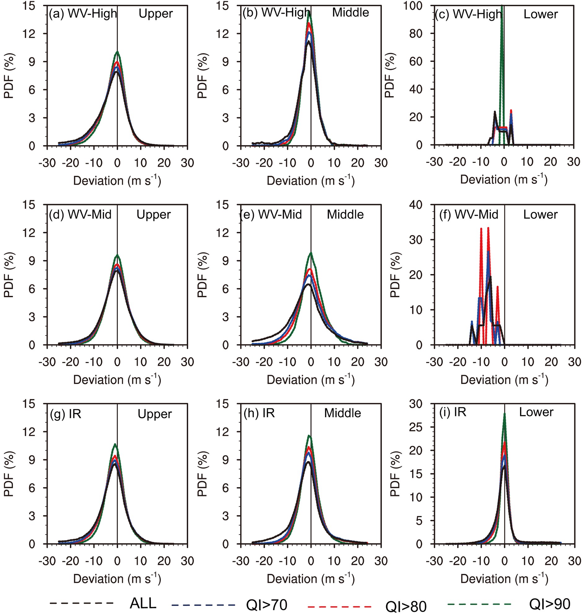 Figure5. PDF of deviation of AMVs derived from (a?c) WV-High, (d?f) WV-Mid and (g?i) IR in the upper layer (above 400 hPa), middle layer (400?700 hPa) and lower layer (below 700 hPa).
Taking the data amount and quality (bias, RMSE and PDF) of the three channels into consideration, AMVs with QI greater than 80 will be extracted from products for subsequent research, and AMVs below 700 hPa in the two water vapor channels will not be assimilated.
Conventional observation data or reanalysis data are often used as reference fields in the observation error statistics. The RMSE is usually regarded as the observation error on the premise that the observation is not related to the reference field (Benjamin et al., 1998; Gao et al., 2012). Most previous studies estimated AMV observation error through direct comparison between AMVs with radiosonde data (Hollingsworth and L?nnberg, 1986; Bormann et al., 2003; Bedka et al., 2008). As radiosonde data are too sparse in terms of spatial and temporal resolution compared to FY-4A AMVs, if selected as reference fields, fewer samples of data pairs could be selected and therefore representative errors would be caused. Therefore, the FNL reanalysis is used as the reference field in this study.
Referring to the layered criterion in the default observation error file from the Weather Research and Forecasting Model Data Assimilation (WRFDA) system and the statistical method used in Cordoba et al. (2017) and Desroziers et al. (2005), the model layer is vertically divided into n layers at an interval of 50 hPa. The number of AMV data at each layer is recorded as


where


Figure 6 shows the AMV observation error profiles for the three channels averaged from 1?30 November 2018. Compared to default observation errors, the new observation errors vary with height obviously. The error profiles of the three channels have similar structure and comparable values above 400 hPa. However, between 700 hPa and 400 hPa, the observation errors of WV-High (


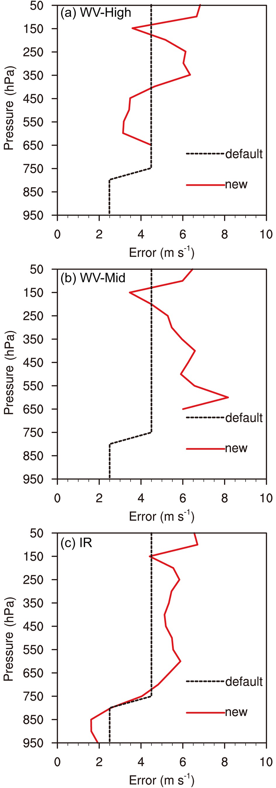 Figure6. Vertical profiles of default observation error (black dotted line) and new observation error (red line) of AMVs for (a) WV-High, (b) WV-Mid and (c) IR (units: m s?1).
In terms of the specific values,


A more accurate observation error value is conducive to a more reasonable estimation of the weight of AMV observations in the process of assimilation, leading to a better 3D wind field analysis. Thus, new observation errors of the three channels will be applied to the subsequent assimilation experiments.
4.1. Model configuration
This study is based on the Rapid-refresh Multi-scale Analysis and Prediction System—Short Term (RMAPS-ST), which runs operationally at the Beijing Meteorological Bureau (Fan et al., 2013; Chen et al., 2014; He et al., 2019; Xie et al., 2019). In RMAPS-ST, the Advanced Research version of the WRF model, version 3.9, and the WRFDA system are employed. Assimilation is performed on a large domain with a grid spacing of 9 km and
The experimental domain is shown in Fig. 7 with the distribution of the main conventional observations at 0000 UTC 1 November 2018. AMVs derived from the WV-High, WV-Mid and IR channels are assimilated in this study by merging with conventional observations. Both the initial and boundary conditions are obtained from the Global Forecast System produced by the National Centers for Environmental Prediction. The Thompson microphysics scheme (Thompson et al., 2008) and RRTMG long- and shortwave radiation scheme (Iacono et al., 2008) are used. In addition, the Kain?Fritsch cumulus parameterization scheme (Kain, 2004) is also adopted in this domain.
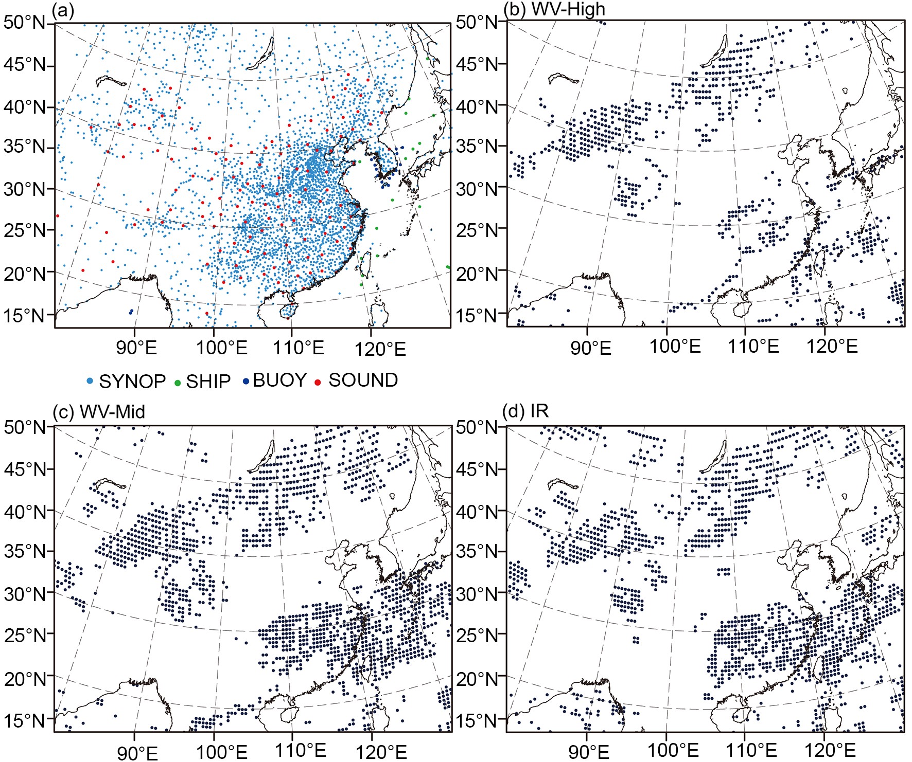 Figure7. Domain of the model and the locations of the (a) main types of conventional observation data, (b) WV-High AMVs, (c) WV-Mid AMVs and (d) IR AMVs (SYNOP denotes surface station observations; SHIP denotes ship observations; BUOY denotes buoy observations, and SOUND denotes radiosonde observations).
2
4.2. Experimental setup
Capability to assimilate AMVs derived from the three channels with new observation errors has been implemented within RMAPS-ST in this study. Five experiments (Table 1) are configured to investigate the added value from the assimilation of FY-4A AMVs on analyses and forecasts with new observation error. Firstly, the control experiment only assimilates the conventional observations (hereafter CTRL). Then, AMVs from WV-High (CONWVh), WV-Mid (CONWVm) and IR (CONIR) are assimilated together with conventional data, respectively. Moreover, an experiment with AMVs from the three channels assimilated simultaneously (CONALL) is added as well. Additionally, to better display the impact of the new observation error on analyses and forecasts, an experiment assimilating three-channel AMVs with default observation error in WRFDA is necessary, and is named CONALL-DEF.| Experiment | Observation error | Assimilation data |
| CTRL | Default value defined in WRFDA | Conventional observations |
| CONWVh | New observation error Rwvh | AMVs from WV-High Conventional observations |
| CONWVm | New observation error Rwvm | AMVs from WV-Mid Conventional observations |
| CONIR | New observation error Rir | AMVs from IR Conventional observations |
| CONALL | New observation error Rwvh, Rwvm and Rir for each channel | Conventional observations AMVs from three channels |
| CONALL-DEF | Default observation error in WRFDA | Conventional observations AMVs from three channels |
Table1. Experiment design schemes.
In the six experiments, partial cycle operation (Hsiao et al., 2012) is adopted at 0000 UTC every day, which means that the initial field of 0000 UTC comes from a 6-h forecast beginning at 1800 UTC of the previous day. Then, the assimilation runs eight times at 0000, 0300, 0600, 0900, 1200, 1500, 1800 and 2100 UTC per day with 3-h cycling. At each analysis time, data within a 3-h window centered on the synoptic time will be ingested and a 24-h forecast will be obtained.
5.1. Data absorption ratio
Table 2 calculates the average proportion of the AMVs absorbed by the assimilation system to the total AMVs used in each assimilation process from experiments with new observation errors first. On average, more than 90% of the data are absorbed in each assimilation cycle, indicating the utilization rate of FY-4A AMVs from the three channels with QI greater than 80 is relatively high. Since observations from radiosondes are obtained twice a day at 0000 UTC and 1200 UTC, the time series of AMV observation minus background (OMB) and AMV observation minus analysis (OMA) of horizontal wind components at 1200 UTC are statistically analyzed in Fig. 8. It can be seen from the time series of OMB (Figs. 8a and c), the U component in FY-4A AMVs is smaller than the background, while the V component is larger than the background. However, the assimilation clearly reduces the deviation between the analysis and observation (Figs. 8b and d), with a more stable time series and a weakened amplitude.| Experiment | Layers (hPa) | ||||||||
| 900?1000 | 800?900 | 800?700 | 700?600 | 600?400 | 400?300 | 300?200 | 200?100 | 100?50 | |
| CONWVh | ? | ? | ? | 99.6 | 99.97 | 99.94 | 99.95 | 99.99 | 99.99 |
| CONWVm | ? | ? | ? | 99.99 | 99.98 | 99.96 | 99.97 | 99.99 | 99.99 |
| CONIR | 97.5 | 98.7 | 99.84 | 99.96 | 99.9 | 99.98 | 99.98 | 99.99 | 99.99 |
| CONALL | 97.5 | 98.7 | 99.79 | 99.89 | 99.93 | 99.96 | 99.96 | 99.97 | 99.99 |
Table2. Average absorption ratios (%) of AMVs in different layers (hPa) from experiments assimilating with new observation errors.
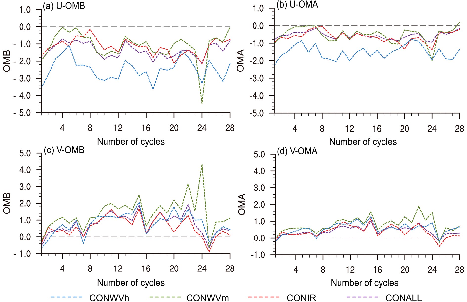 Figure8. Time series of the (a, c) OMB and (b, d) OMA statistics of the U and V components for assimilating FY-4A AMVs at 1200 UTC from the experiment assimilating FY-4A AMVs with new observation errors.
Moreover, the OMB sequence obtained by simultaneous assimilation of AMVs from the three channels is stable with no obvious outliers under the mutual restriction of data from the three channels. Also, the OMA is closer to 0 than that of the single-channel assimilation experiments, which means that the wind analysis obtained from the multi-channel assimilation experiment is better than that from the single-channel assimilation experiments.
2
5.2. Verification for single-channel assimilation
The RMSEs for the analysis and forecast against sounding observations are calculated by the Model Evaluation Tools (MET) verification package (Kirby, 2004), which is designed to be a highly configurable, state-of-the-art suite of verification tools. MET provides a variety of verification techniques, including standard verification scores comparing gridded model data obtained from the WRF modeling system with point-based observations.3
5.2.1. Wind fields
Since the AMV products mainly contain wind field information, only horizontal wind components (U and V) are discussed. Figure 9 shows the vertical profiles of the mean analysis RMSEs for horizontal winds (U, V) (solid lines) and the forecast RMSEs at t+6 h (dashed lines) and t+24 h (dotted lines) of CTRL and the experiments assimilating the single-channel AMVs. The experiments assimilating FY-4A AMVs achieve comparable analysis with CTRL, and even slightly inferior to CTRL, especially for the U component at 300 hPa, which may be related to the sparse resolution of the reference radiosonde observations. Figure9. Averaged vertical RMSE pro?les for analyses and 6-h and 24-h forecasts in comparison with radiosonde data for CTRL and single-channel assimilation experiments.
After 6-h forecasts, the experiments assimilating FY-4A AMVs reduce the RMSEs in wind fields compared to CTRL. Positive effects mainly occur in the upper and middle layers, which is in accordance with the layer where FY-4A AMVs are distributed (Fig. 1d). Besides, among the three channels, the assimilation of WV-High AMVs produces more obvious improvement, while AMVs from the other two channels have a relatively weak effect on the 6-h forecast. After 24-h forecasts, the RMSEs of the horizontal wind components become larger, and the advantage of assimilating FY-4A AMVs gradually diminishes, but still appears in the U component below 500 hPa and V component above 500 hPa. Moreover, AMVs from the IR channel have a clearer positive impact on the 24-h forecast than that from the two water vapor channels.
At the same time, the mean RMSEs in the three layers for different experiments are calculated for various lead times. The results (Fig. 10) show that the assimilation of FY-4A AMVs reduces the RMSEs of the U and V components in the upper layer, and the improvement can even be seen in the 24-h forecast. Focusing in the middle and lower layers, AMVs from the two water vapor channels produce little positive effect because of no observations below 700 hPa. However, the assimilation of AMVs from IR improves the forecast of the V component in the middle layer, and improvement of the horizontal components in the lower layers in CONIR is gradually shown after 18 h of forecasting.
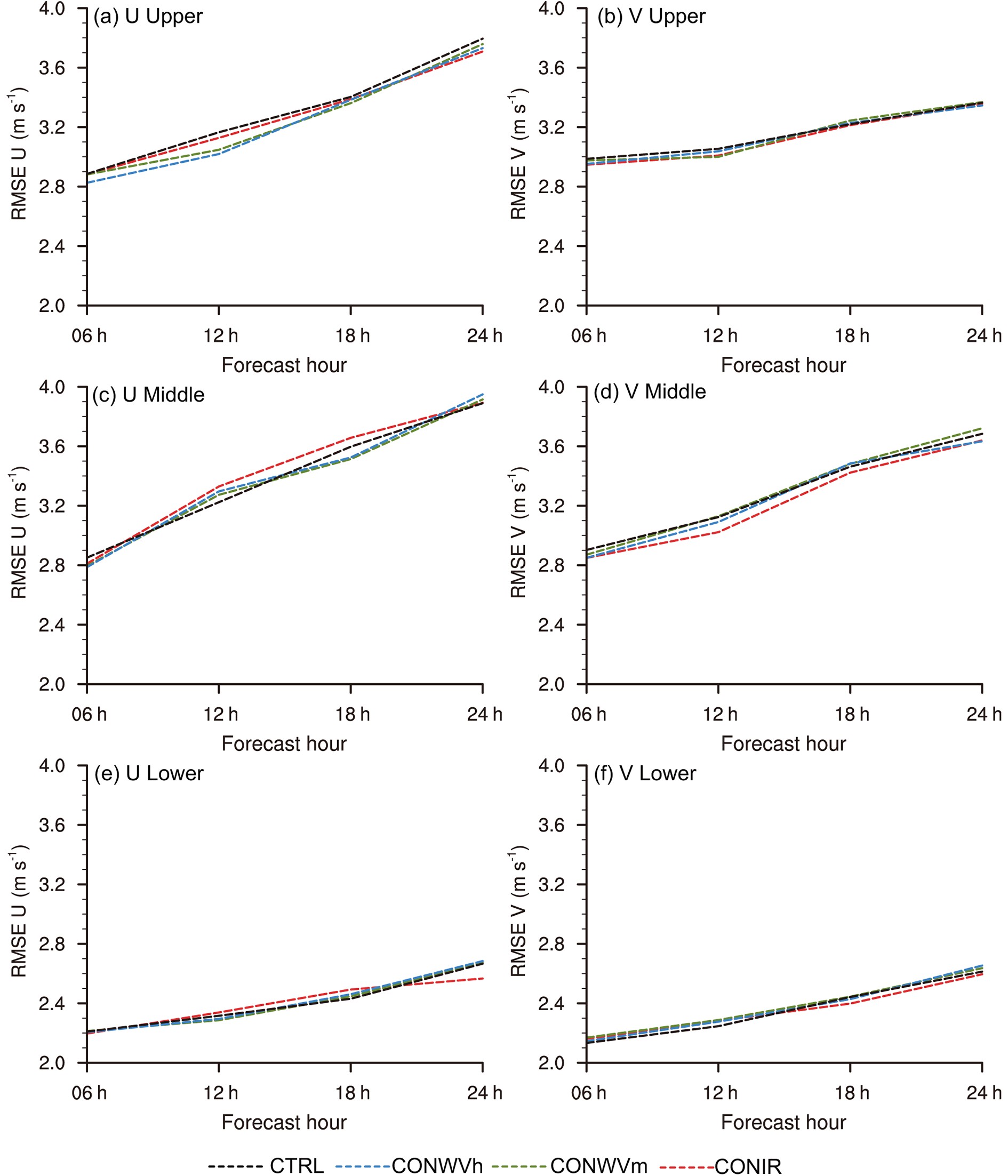 Figure10. Average RMSEs at different lead times for the (a, b) upper layer (above 400 hPa), (c, d) middle layer (400?700 hPa) and (e, f) lower layer (below 700 hPa) for the CTRL and single-channel assimilation experiments.
In terms of the vertical distribution of FY-4A AMVs, a large number of AMVs from the three channels concentrate at 300 hPa, while only AMVs from IR are available below 700 hPa. Figure 11 displays the trend of RMSEs at 300 hPa and 700 hPa with lead time. It is clear that AMVs derived from the two water vapor channels have an advantage in improving the forecast in the upper layer, especially the data from WV-High, while AMVs from IR can produce noticeable improvement in the lower layer after 12 h of forecasting.
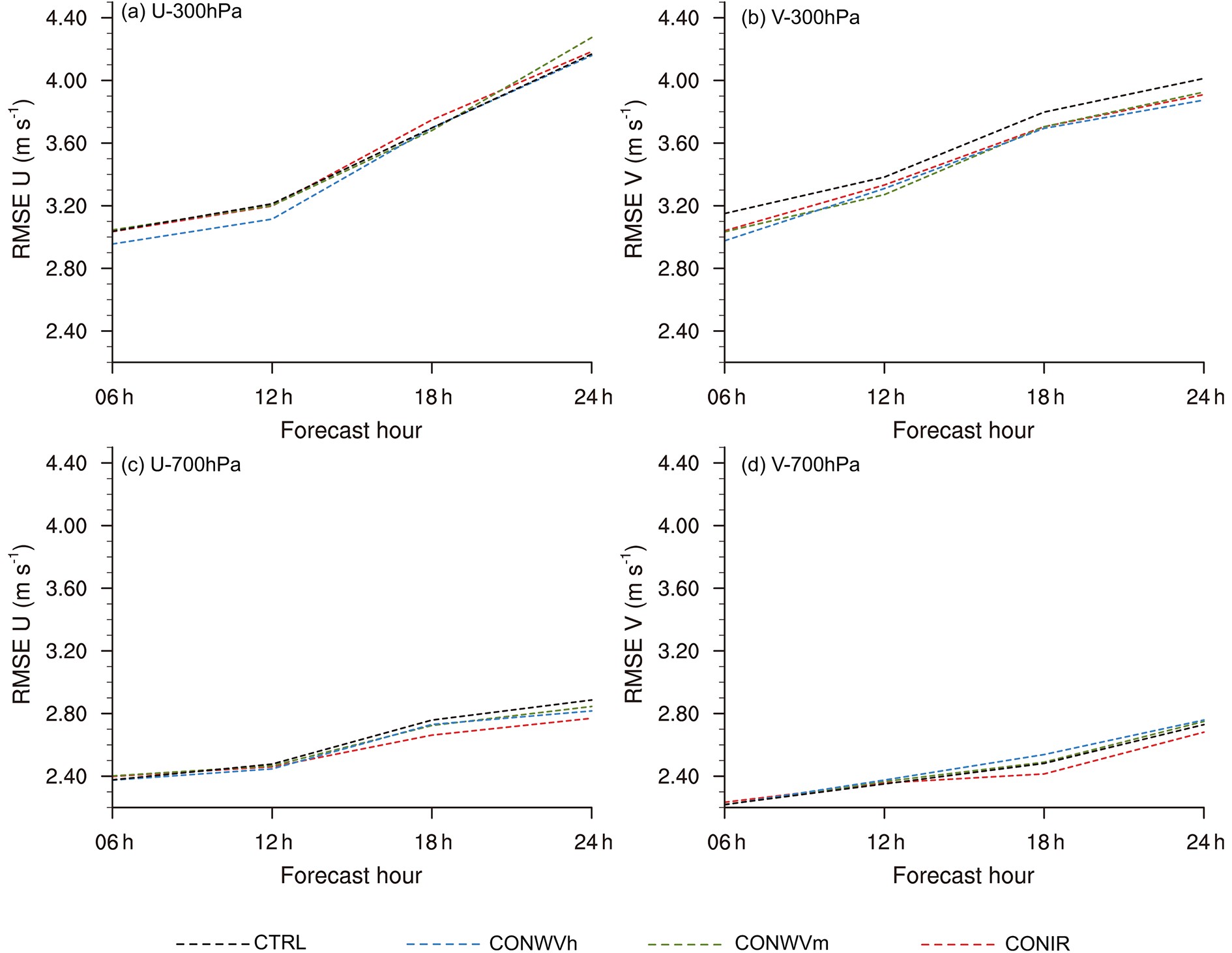 Figure11. RMSEs at 300 hPa and 700 hPa at different lead times for the CTRL and single-channel assimilation experiments.
3
5.2.2. Precipitation forecast
Several precipitation processes occur during the research period, so the impact of FY-4A AMVs on the precipitation forecasting skill is evaluated. The bias score (BS), threat score (TS), probability of detection (POD), and false alarm ratio (FAR) (formulae shown in Table 3) are used. The closer the BS, TS and POD are to 1, the higher the prediction accuracy of precipitation; and the smaller the FAR, the fewer false alarms in the precipitation forecast. The precipitation data for comparison are the hourly observations from surface stations provided by the CMA.| Index | Formula |
| Bias Score (BS) | (hits + false alarms)/(hits + misses) |
| Threat Score (TS) | hits/(hits + false alarms + misses) |
| Probability of Detection (POD) | hits/(hits + misses) |
| False Alarm Ratio (FAR) | false alarms/(hits + false alarms) |
Table3. Four statistical indices for rainfall forecast skill.
The average TS, BS, POD and FAR for the 6-h accumulated precipitation with thresholds of 0.1 mm, 1.0 mm, 5.0 mm 10.0 mm and 25.0 mm are shown in Fig. 12. Compared to CTRL, the assimilation of the FY-4A AMVs results in a decrease in BS for 6-h accumulated precipitation with intensity between 1.0 mm and 10.0 mm, and CONIR has the smallest values. Besides, the average TS and POD in CONWVm and CONIR show a slight improvement in precipitation with thresholds between 1.0 mm and 10.0 mm. In addition, the FAR of the experiments assimilating FY-4A AMVs decrease when compared to CTRL, and CONIR produces the lowest FAR value. However, owing to the actual intensity of the 6-h accumulated precipitation from these rainfall events being lower than 25.0 mm, the added AMVs lead to an under-prediction with the threshold of 25.0 mm, overall.
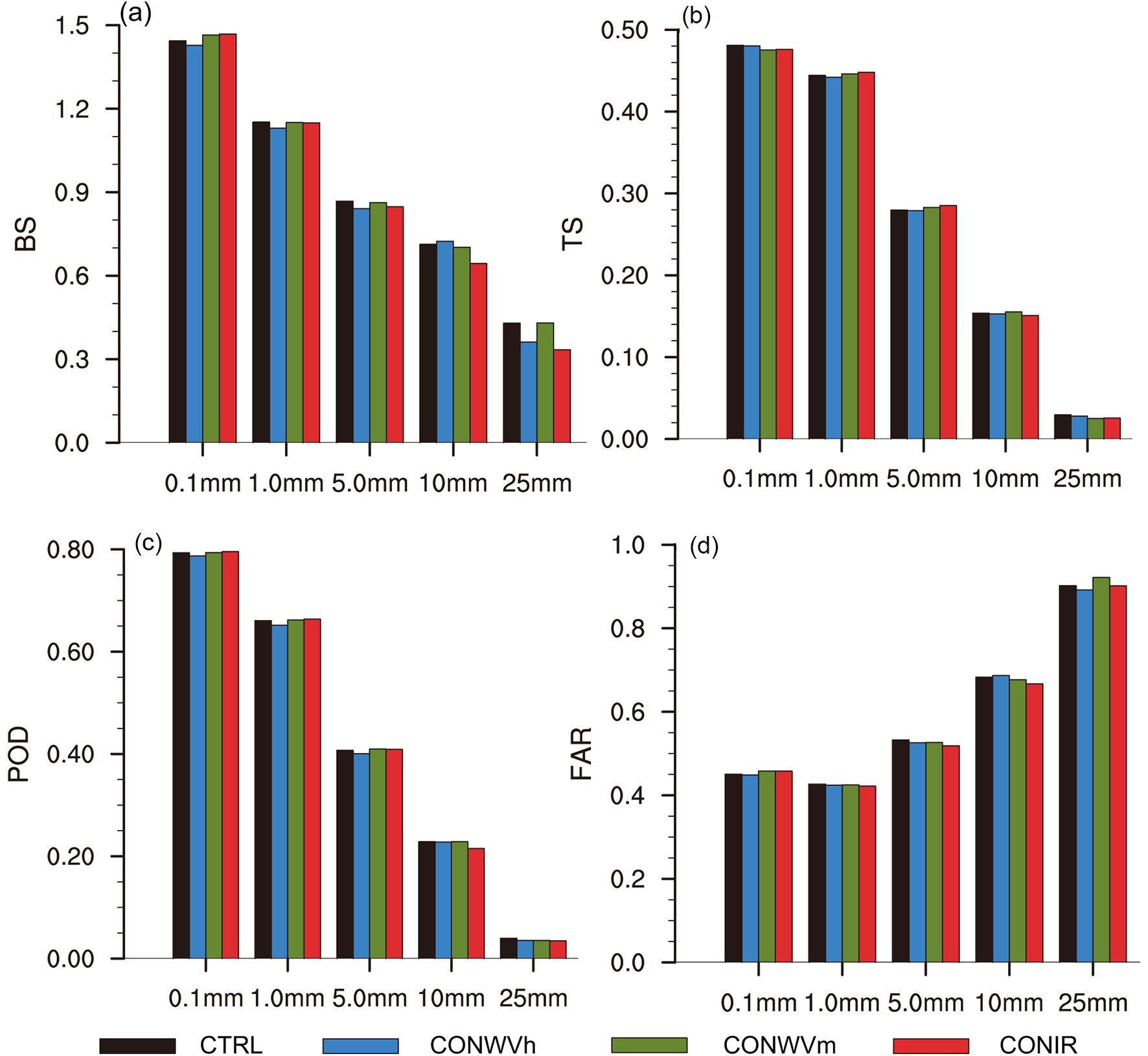 Figure12. Average BS (a), TS (b), POD (c) and FAR (d) for the 6-h accumulated precipitation with different thresholds for the CTRL and single-channel assimilation experiments.
Generally, the results suggest that AMVs derived from the IR channel produce the largest improvement among the three channels. The reason may be that the precipitation intensity of these processes during the experiment is relatively weak and the vertical development relatively low. As a result, the wind of the lower layer in the IR channel has a positive impact on the precipitation.
2
5.3. Verification for multi-channel assimilation
Through the above discussion of the impact of assimilating single-channel AMVs on the analysis and forecasts, it can be concluded that the FY-4A AMVs from the water vapor channels mainly improve the wind field in the upper layer. Meanwhile, assimilating AMVs from IR has a slightly positive impact in the middle and lower layers. Next, to combine the advantages of the three channels, FY-4A AMVs from the three channels are simultaneously assimilated, and the impact on the forecast further analyzed.Figure 13 displays the average RMSEs of the analysis and forecasts for the horizontal winds (U, V) of CTRL, CONALL and CONALL-DEF. Similar to Fig. 9, the assimilation of FY-4A AMVs derived from the three channels produces analyses a little inferior to that of CTRL, especially for the upper layer where a large number of AMVs are distributed, which is due to the rough spatial resolution of the radiosonde data. Also, the improvement from assimilating FY-4A AMVs will be seen after integrating for several hours. For example, the differences between the RMSEs of the experiments assimilating AMVs and that of CTRL decrease after six hours of model integration, and their RMSEs are relatively smaller than those of CTRL for the V component under 400 hPa. For the 24-h forecast, the RMSEs of U and V in CONALL and CONALL-DEF are smaller than those in CTRL at almost all levels. The main advantage of assimilating FY-4A AMVs in the U component gradually shifts from the upper layer to the middle and lower layer, while the improvement of the V component is still shown in the upper layer.
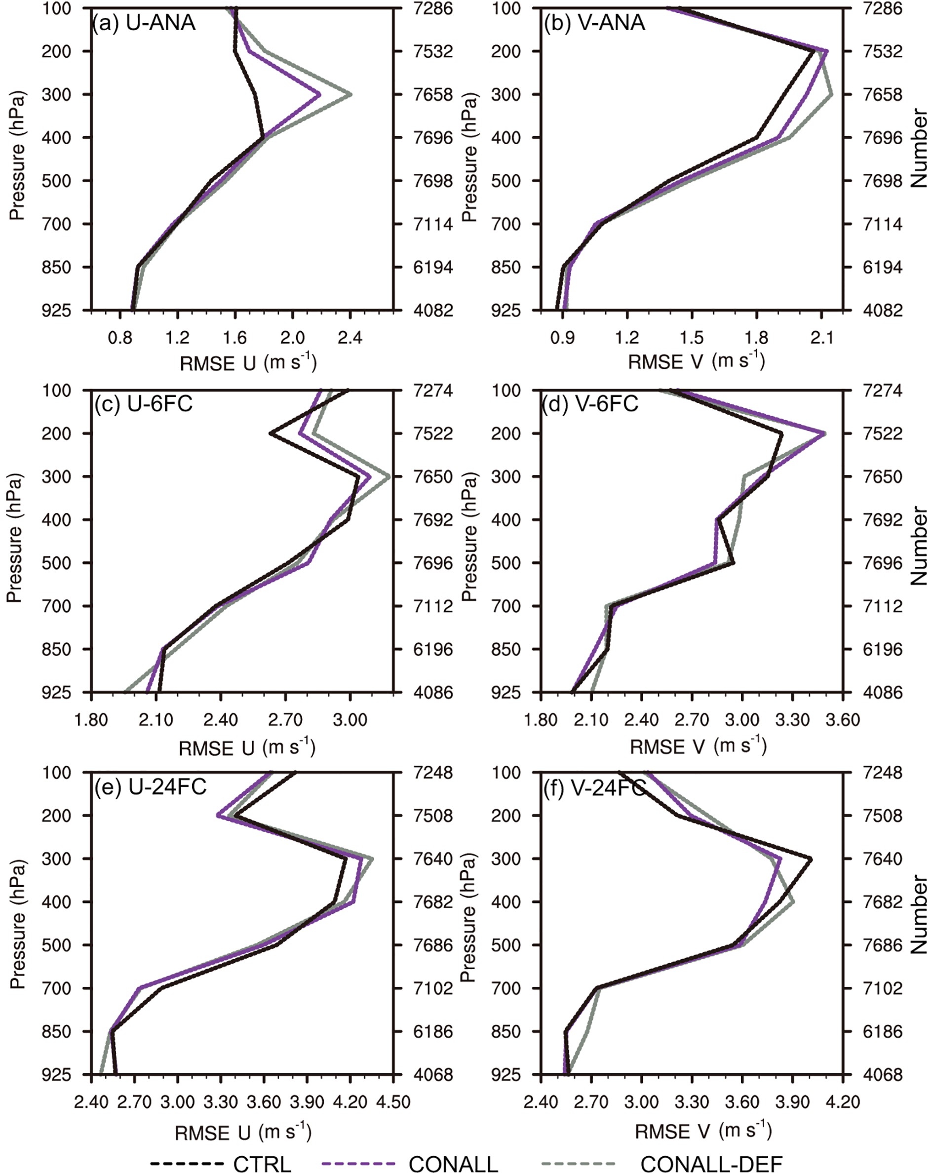 Figure13. Averaged vertical RMSE pro?les for analyses and 6-h and 24-h forecasts in comparison with radiosonde data for CTRL, CONALL and CONALL-DEF.
In addition, Fig. 13 also shows the impact of different observation errors on assimilation and prediction results. As can be seen from the RMSE profiles, when compared to CONALL-DEF (gray lines), assimilating FY-4A AMVs with new observation errors (purple lines) can clearly reduce the RMSEs of the horizontal wind components in almost all layers both in the analyses and 6-h and 24-h forecasts, which can serve as a reference for the significance of estimated observation error in new observation datasets.
Besides, according to the precipitation forecasting skill scores displayed in Fig. 14, except for the threshold of 0.1 mm, CONALL results in a decrease of BS and FAR when compared to CTRL. Moreover, the average TS and POD in CONALL show a slight improvement for precipitation with thresholds between 1.0 mm and 10.0 mm, which is similar to the result obtained in the single-channel assimilation.
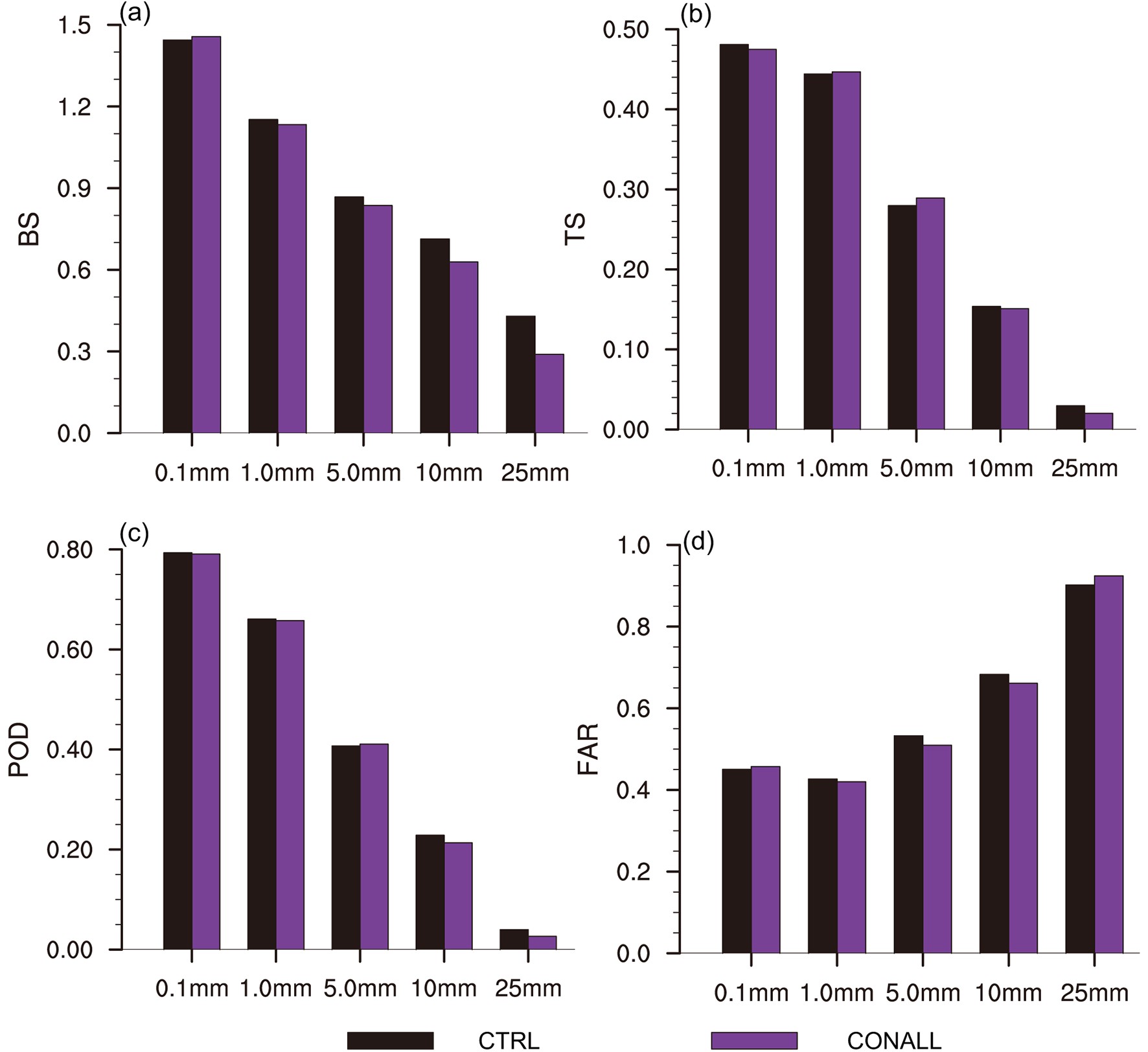 Figure14. Average BS (a), TS (b), POD (c) and FAR (d) for the 6-h accumulated precipitation with different thresholds for CTRL and CONALL.
(1) FY-4A AMVs derived from the two water vapor channels are concentrated in the upper and middle layers, especially between 400 hPa and 200 hPa, while AMVs from IR have a maximum total number in the upper and lower layers. In addition, AMVs derived from the three channels show relatively normal PDF distributions of deviation from the reference field in the upper and middle layers, as do FY-4A AMVs in the lower layer derived from the IR channel.
(2) Observation errors of FY-4A AMV products have obvious vertical structures. The profiles of the three channels above 400 hPa are similar in structure and are quantitatively comparable. Between 400 hPa and 700 hPa, the observation errors of WV-High increase with height, while those of WV-Mid and IR decrease with height.
(3) The one-month single-channel data assimilation cycling and forecasting experiments demonstrate that assimilating FY-4A AMVs improves wind forecasts. Moreover, AMVs from WV-High produce more apparent improvement in the wind field in the upper layer, and AMVs from IR can achieve more obvious positive effects in the lower layer. Furthermore, assimilating AMVs from IR produces higher skill scores for medium and moderate precipitation than the other channels owing to its good quality of data in the lower layer.
(4) Simultaneous assimilation of FY-4A AMVs from the three channels combines the advantages of assimilating the three individual channels to improve the forecasts in the upper, middle and lower layers at the same time. Moreover, simultaneous assimilation has an obvious positive impact on the precipitation forecast with thresholds between 1.0 mm and 10.0 mm.
Considering that the AMV products derived from the FY-4A satellite are still being studied, more comprehensive and detailed comparisons and evaluations should be conducted in the future by combining the AMV products derived from other satellites, such as those from Himawari-8. In addition, stricter quality-control procedures for FY-4A AMVs should be implemented to reduce the correlation between AMVs. Moreover, the experimental scheme of simultaneous assimilation of FY-4A AMVs of the three channels still needs to be improved, and duplication of the AMVs between different channels for assimilation should be further considered.
Acknowledgements. This research was funded by the National Key Research and Development Plan (Grant No. 2018YFC1507105). We wish to thank Dr. Xiaohu ZHANG from the National Satellite Meteorological Center of China for providing the AMV data and other relevant help. We also thank the Editor and reviewers for their comments and suggestions for improving the manuscript.
