Boru MAI^1,τ,,,
Xuejiao DENG¹,
Fang ZHANG²,
Hao HE³,
Tian LUAN⁴,
Fei LI¹,
Xia LIU⁵

Corresponding author: Boru MAI,maibr@gd121.cn;

1.Institute of Tropical and Marine Meteorology, China Meteorological Administration, Guangzhou 510640, China
2.College of Global Change and Earth System Science, Beijing Normal University, Beijing 100875, China
3.Department of Atmospheric and Oceanic Science, University of Maryland, College Park, MD 20742, USA
4.Chinese Academy of Meteorological Sciences, Beijing 100081, China
5.Guangzhou Meteorological Observatory, Guangzhou 511430, China
Manuscript received: 2019-11-13
Manuscript revised: 2020-02-13
Manuscript accepted: 2020-02-24
Abstract:Mole fractions of atmospheric CO₂ (XCO₂) have been continuously measured from October 2014 to March 2016 at the Guangzhou Panyu Atmospheric Composition Site (23.00°N, 113.21°E; 140 m MSL) in the Pearl River Delta (PRD) region using a cavity ring-down spectrometer. Approximately 66.63%, 19.28%, and 14.09% of the observed values were filtered as background, pollutant source, and sink due to biospheric uptake, respectively, by applying a robust local regression procedure. Their corresponding mean values were 424.12 ± 10.12 ppm (×10^?6 mol mol^?1), 447.83 ± 13.63 ppm, and 408.83 ± 7.75 ppm. The background XCO₂ levels were highest in spring and winter, moderate in autumn, and lowest in summer. The diurnal XCO₂ was at a minimum from 1400–1600 LST (Local Standard Time) and a maximum at 0500 LST the next day. The increase of XCO₂ in spring and summer was mainly associated with polluted air masses from south coastal Vietnam, the South China Sea, and the southeast Pearl River Estuary. With the exception of summer, airflow primarily from marine regions southeast of Taiwan that passed over the Pearl River Estuary had a greater impact on XCO₂, suggesting an important potential source region.
Keywords: background CO₂ mole fraction,
Pearl River Delta region,
potential source region
摘要:城市群大气CO₂是全球碳循环的重要组成部分，对全球增温以及区域气候变化具有显著作用。相对于背景区域而言，人们对城市地区大气CO₂的了解比较有限。探明城市群大气CO₂的本底/非本底特征及潜在源区，对约束和提高大气CO₂的模式评估具有重要意义。2014年10月至2016年3月期间，利用光腔衰荡技术在广州番禺大气成分站（23.00°N, 113.21°E; 140 m MSL）连续在线观测了大气CO₂的摩尔分数（XCO₂）。利用平均移动过滤法筛分了观测数据的本底、非本底信号。采用72小时后向轨迹聚类分析了大气CO₂的长距离输送特征，结合潜在来源贡献算法区分了CO₂的潜在源区。结果表明：在观测期间，大约66.63%, 19.28%和14.09%的CO₂分别为本底值、污染源以及由植被吸收引起的吸收汇，其浓度分别为424.12±10.12 ppm (×10^?6 mol mol^?1), 447.83±13.63 ppm 和 408.83±7.75 ppm。大气CO₂的本底浓度在春、冬季最高，秋季居中，夏季最低，其日变化均在1400–1600（北京时）出现最低值，在次日的0500时达到最高值。春、夏季XCO₂的抬升主要受到了来自越南南部、南海以及珠江口东南部海域污染气团的影响。除夏季外，其他季节来自台湾东南部海域再迂回珠江口的气团对XCO₂有显著作用，是重要的潜在源区。
关键词:本底CO₂的摩尔分数,
珠三角区域,
潜在源区

HTML

--> --> -->

Carbon dioxide (CO₂) is the most important greenhouse gas, contributing more than 60% of the total radiative forcing of the long-lived greenhouse gases (IPCC, 2013). Since the 1750s, tropospheric CO₂ mixing ratios have been increasing, rising to approximately 396.0 ± 0.1 ppm in 2013, according to observations at background stations (WMO, 2014). This increase derives mainly from the burning of fossil fuels and land-use changes (Houghton, 2003; Peters et al., 2012). Natural sources of CO₂ include biomass burning and oxidation of natural volatile organic compounds (VOCs). Trends in the atmospheric burden of CO₂ may also directly affect isoprene emissions by involving competition for substrates between terpenoid biosynthesis and cytosolic carbon metabolism in several plant taxa (Rosenstiel et al., 2003). Note that isoprene is a VOC emitted by vegetation. It plays a significant role in modulating atmospheric composition, including the concentrations of ozone and particulate matter. To enhance our understanding of the carbon cycle, and even the relationship between CO₂ and isoprene emissions, which has substantial implications for air quality (Young et al., 2009; Tai et al., 2013), it is crucial to quantify atmospheric CO₂ variations (Tans et al., 1990; Peters et al., 2007). Since the late 1950s, long-term measurements of atmospheric CO₂ concentration have been systematically conducted at many locations around the globe (Keeling et al., 1976; Conway et al., 1994; Keeling, 2008). Studies show that the current global CO₂ observation network constrains emissions estimates to continental scales (Thompson et al., 2009; Chevallier et al., 2011). Anthropogenic emissions, however, are largely concentrated in urban areas. Net fluxes per unit area in urban regions greatly exceed those of forests (Briber et al., 2013).
The possibility of monitoring anthropogenic greenhouse gas emissions in urban areas is only beginning to be explored (Mays et al., 2009; Strong et al., 2011; Newman et al., 2012). It has been reported that urban areas are now home to more than half the world’s population, and are estimated to contribute over 70% of global energy-related CO₂ emissions (Rosenzweig et al., 2010). Therefore, in addition to focusing on the characteristics of global/regional background CO₂ concentrations, it is important to understand the behavior of CO₂ in urban areas and, in particular, emission source regions that contribute disproportionately to the atmosphere’s anthropogenic greenhouse gas burden (Gurney et al., 2009; Rayner et al., 2010).
A large number of studies have been carried out by filtering high-resolution CO₂ data in order to quantify the behavior of CO₂ from source to sink regions (Keeling, 2008; Zhang and Zhou, 2013; Luan et al., 2015; Zhang et al., 2015). Overall, these methods include the robust extraction of baseline signal (REBS) (Ruckstuhl et al., 2012), the surface winds and diurnal variations (SWDV) (Bousquet et al., 1996), the CO tracer method (Tsutsumi et al., 2006), and the Fourier transform axiom (FTA) (Masarie and Tans, 1995). Recently, a comparison study was made between the REBS and the SWDV methods using CO₂ data at the Longfengshan (LFS) WMO/GAW regional station in China (Luan et al., 2015). The results showed that the data acquired by the SWDV method during the day, when the airflow was from the southwest, and the data gathered by the REBS method during calm conditions, were occasionally misidentified as background events. Zhang and Zhou (2013) and Zhang et al. (2013, 2015) developed a new method for extracting atmospheric CO₂ sources/sinks and background information known as Moving Average Filtering (MAF). They also compared and analyzed the performances of MAF, REBS, and FTA using the high-resolution CO₂ concentration data from Waliguan (WLG) station, and suggested that the three methods could reasonably extract anthropogenic-influenced episodes, although only the MAF method could adequately identify the episodes due to terrestrial CO₂ fluxes.
To the best of our knowledge, the carbon sources and sinks of CO₂ differ significantly, as reflected in the trends, intensities, and regional distributions obtained by various studies (Le Quéré et al., 2009; Piao et al., 2009). In order to improve the calculation of regional CO₂ sources and sinks, one possible solution is to extract the dynamic variation of real-time sources and sinks from the long-term continuous observational data, so as to estimate the strength of the carbon sources/sinks on the regional scale in combination with an atmospheric inversion model (Prinn et al., 2000; Reimann et al., 2005). Another approach is to utilize high-frequency data. Using this method, the regional/local influences and pollution transport characteristics can be derived by combining them with meteorological data, after which source/sink strengths can be estimated using inversion models over a regional scale (Zhang et al., 2013).
The Pearl River Delta (PRD) region is the largest and most important economic zone in China, in which an open-door policy and drastic economic reform took place in the 1980s. Due to the rapid growth of industrialization and urbanization over the past several decades, the emission amounts and growth rates of CO₂ have increased dramatically worldwide, particularly in the PRD of China (Mai et al., 2014), which has become one of the fastest developing regions in the world. In order to expand the observations of greenhouse gases in the PRD region, a cavity ring-down spectroscopy (CRDS) analyzer (G2301, Picarro, Inc., USA) was installed at the Guangzhou Panyu Atmospheric Composition Site (GPACS) in 2014. Since then, first-hand observations of the XCO₂ (mole fractions of atmospheric CO₂) levels in this region have been acquired. The goals of this study are to: (1) determine the background and non-background XCO₂ in the PRD region using high-resolution in-situ observation data of CO₂ from the GPACS; (2) analyze the characteristics of the long-distance transport of atmospheric CO₂ using 72-h backward trajectories; and (3) examine the potential source regions of CO₂ in the PRD using the Weight Potential Source Contribution Function (WPSCF). Section 2 describes the datasets and methods. Section 3 presents results and discussion. Conclusions are provided in section 4.

Measurements were taken from October 2014 to March 2016 at GPACS, which is the main station in the observation network for atmospheric composition in the PRD. The station is located on the peak of Dazhengang Mountain in the town of Nancun, Panyu district of Guangzhou City, in the PRD region (23.00°N, 113.21°E; 140 m MSL) (Fig. 1). Sampling was done at a height of 8 m above the surface using a G2301 CO₂/CH₄/H₂O analyzer (Picarro, Inc., USA). This instrument adopts the Wavelength-Scanned Cavity Ring Down Spectroscopy (WS-CRDS) technique, with a CO₂ measurement accuracy of < 0.05 ppm·(5 min)^?1, a maximum peak drift value of 0.5 ppm month^?1, and a measurement interval of < 5 s. The air sample is filtered by a 7-μm filtering membrane before entering the analyzer. The instrument is provided with a water vapor calibration algorithm; therefore, the samples do not need to be dried. However, to eliminate the possible interference of water vapor on the observation results, air samples are subjected to a cold trap for water removal at a temperature of ?50°C prior to entering the sample selection valve. In order to ensure that the gas in the glass tube of the cold trap is in a flowing state so as to minimize the influence of “dead volume,” a two-stage pressure relief device is positioned at the back of the glass tube, with a flow rate of 250 mL min^?1. Furthermore, an eight-port sample selection valve is used for selecting and analyzing the air or standard gas. Additionally, a high-precision mass flow controller is placed in front of the analyzer in order to stabilize the air samples (Fang et al., 2011; Zang et al., 2011).
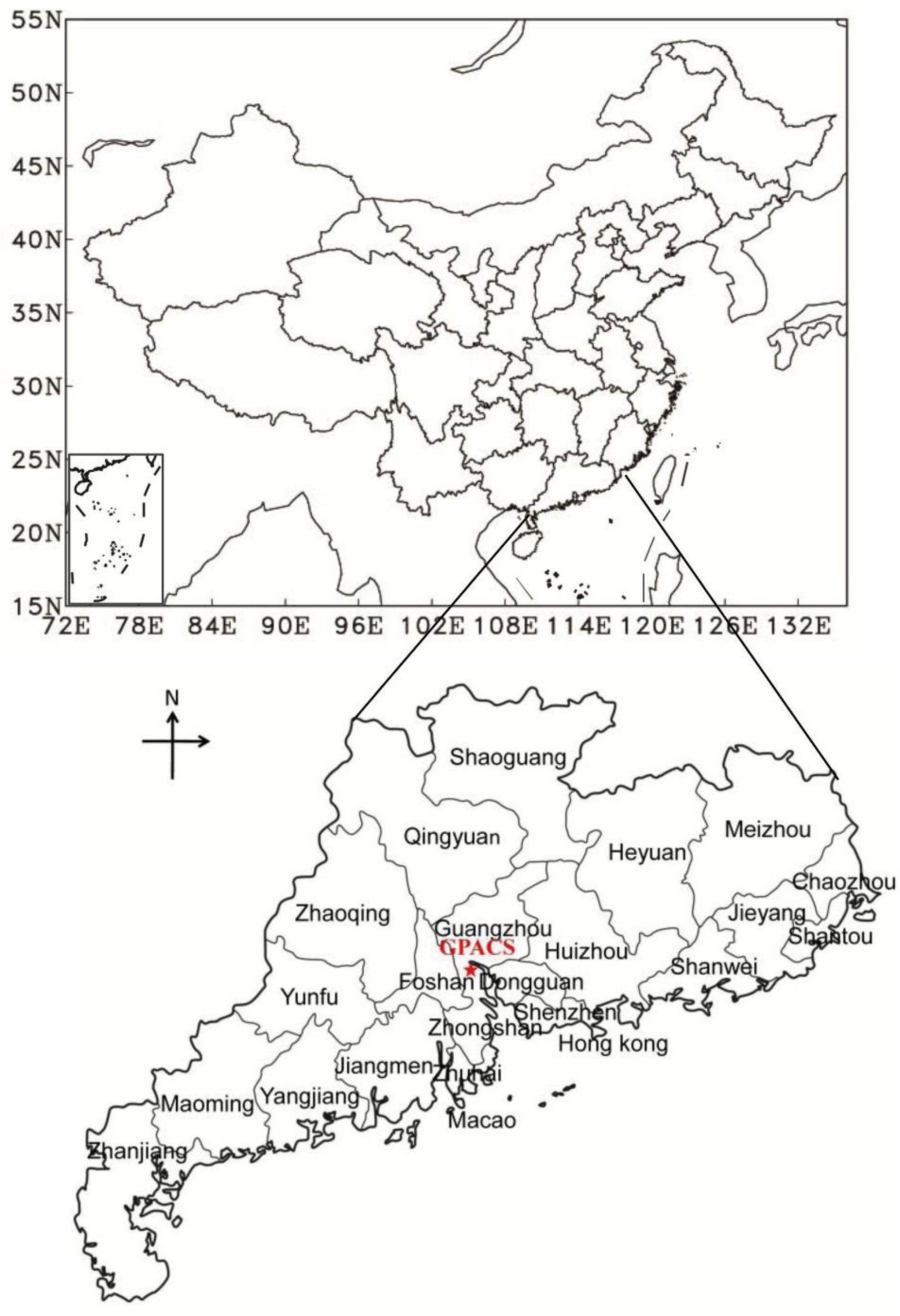Figure1. Location of GPACS.


Calibration was performed once every two weeks; each time the standard gas was analyzed for 5 min. The standard gas was supplied by the Greenhouse Gas Laboratory of the Chinese Academy of Meteorological Sciences, and was traceable to the WMO primary standard gas. Figure 2 illustrates the differences between the measured and assigned values of the standard gas during the observation period. The average mean of the absolute differences was 0.03 ± 0.02 ppm, with 97.56% of the differences < 0.1 ppm, proving that the measurement accuracy met the compatibility goal of the WMO/GAW (0.1 ppm for CO₂ in the Northern Hemisphere). The CO₂ observational data were calculated as 1-min averages, and quality control was carried out in conjunction with the observational record in order to reject abnormal values during instrument failure, maintenance, the influence of human activities, and so on. This process identified approximately 83% of the data as valid.
Figure2. Differences between measured and assigned values of standard gas during the observation period.


The background/non-background data were determined by the MAF statistical method, which has been applied to ambient CO₂ baseline calculation at WLG (Zhang et al., 2015). The basic assumption is that the concentration of CO₂ in well-mixed air should not change much during a short period. Details of this method are described in Zhang et al. (2013), and depicted in Fig. 3. Briefly, changes in XCO₂ > 0.3 ppm from one hour to the next were deemed to be affected by local sources or sinks and were rejected. The criteria of 0.3 ppm was in accordance with the value used at WLG station (Zhang and Zhou, 2013), but it was higher than some extremely remote monitoring sites, such as the South Pole, Antarctica, where the criteria was as low as 0.1 ppm (Gillette et al., 1987). A two-week work window was then used for the remaining data, in which the maximum or minimum values were removed. The remaining data over the work window were smoothed using a moving average curve fit approach. At this point, the first hourly value that was higher/lower than twice the standard deviation (σ) of the average of the curve would be labeled as pollution source/sink data. By contrast, the data within 2σ of the spline were flagged as background values. Finally, the process was moved to another two-week period for the filtering of the second hourly data.
Figure3. The process of MAF.


HYSPLIT-4 (the Hybrid Single Particle Lagrangian Integrated Trajectory model) (Draxler and Rolph, 2003), developed by NOAA (National Oceanic and Atmospheric Administration) for the study of atmospheric transfer and diffusion, has been widely applied in analyzing the transport and dispersion of air pollutants. We adopted this model in order to investigate the influence of the long-distance transport of air masses on the XCO₂ levels at GPACS, and to identify the potential source regions of CO₂. The meteorological data (ftp://arlftp.arlhq.noaa.gov/pub/archives/gdas1) were from the global reanalysis data of the NCEP (National Centers for Environmental Prediction). The CO₂ data from October 2014–March 2016 were analyzed using trajectory statistics. Three-day (72-h) back trajectories originating at 0000, 0600, 1200, and 1800 UTC were calculated, with the arrival height of the trajectories being 500 m above the surface.
The potential source region of CO₂ was determined by PSCF, which is a useful tool for calculating the probability density of the residence times of an air parcel over a given geographical area prior to its arrival at the measurement site (Ara Begum et al., 2005). In this study, the geographic region (10°–40°N, 90°–130°E) was divided into grid cells (using indices i and j to define the location of grid cells), with a spatial resolution of 0.5° × 0.5° (500 m above the surface). The ${\rm{PSC}}{{\rm{F}}_{i,j}}$ reflects the probability that any given cell can be related to an increase of CO₂ and is defined as
where ${n_{i,j}}$ denotes the number of trajectories that pass through the i,jth cell, and ${m_{i,j}}$ represents the number of trajectories resulting in CO₂ values that exceed the background value. Cells related to the high values of ${\rm{PSC}}{{\rm{F}}_{i,j}}$ are the potential source areas (Polissar et al., 1999). Since the ${\rm{PSC}}{{\rm{F}}_{i,j}}$ is a ratio of ${m_{i,j}}$ and ${n_{i,j}}$, relatively small ${n_{i,j}}$ values, which are often related to sparse trajectory coverage of the more distant grid cells, may result in ${\rm{PSC}}{{\rm{F}}_{i,j}}$ with high uncertainty. In order to alleviate this ambiguity, the ${\rm{PSC}}{{\rm{F}}_{i,j}}$ values were multiplied by an arbitrary weight function ${W_{i,j}}$ to better reflect the uncertainty in the values of these cells (Polissar et al., 1999). For large values of ${n_{i,j}}$, the calculated ${\rm{PSC}}{{\rm{F}}_{i,j}}$ would be more statistically stable. Similar to previous studies (Fang et al., 2016; Zhang et al., 2013), the weight function factor ${W_{i,j}}$ in this investigation was defined as
The ${\rm{WPSC}}{{\rm{F}}_{i,j}}$ was expressed as

2

-->

3.1. Background value filtering of atmospheric CO₂ mole fractions in the PRD region

The background XCO₂ used in this study refers to the value when the atmosphere is well mixed and not affected by regional pollutant sources/sinks. Figure 4 shows selected XCO₂ data from GPACS. Approximately 66.63%, 19.28%, and 14.09% of the hourly valid data were classified as background, pollutant source, and absorption sink values, respectively. It has been reported that the background concentration data of CO₂ at the WLG station accounted for ~70% of the valid data (Zhang and Zhou, 2013), and the proportion at the LFS site accounted for 30.7%–58.9%, depending on the filtering method (Luan et al., 2015). The high percentages of non-background data in this study suggest large impacts from local or regional sources and sinks at GPACS. The mean values of background, pollutant source, and absorption sink XCO₂ were 424.12 ± 10.12 ppm, 447.83 ± 13.63 ppm, and 408.83 ± 7.75 ppm, respectively. The fluctuation of all the observed XCO₂ values was higher, with the hourly amplitude being 153.68 ppm, while the fluctuation of background CO₂ was lower (~56.17 ppm), indicating that the atmospheric CO₂ in the PRD region is strongly affected by regional or local emission sources and absorption sinks.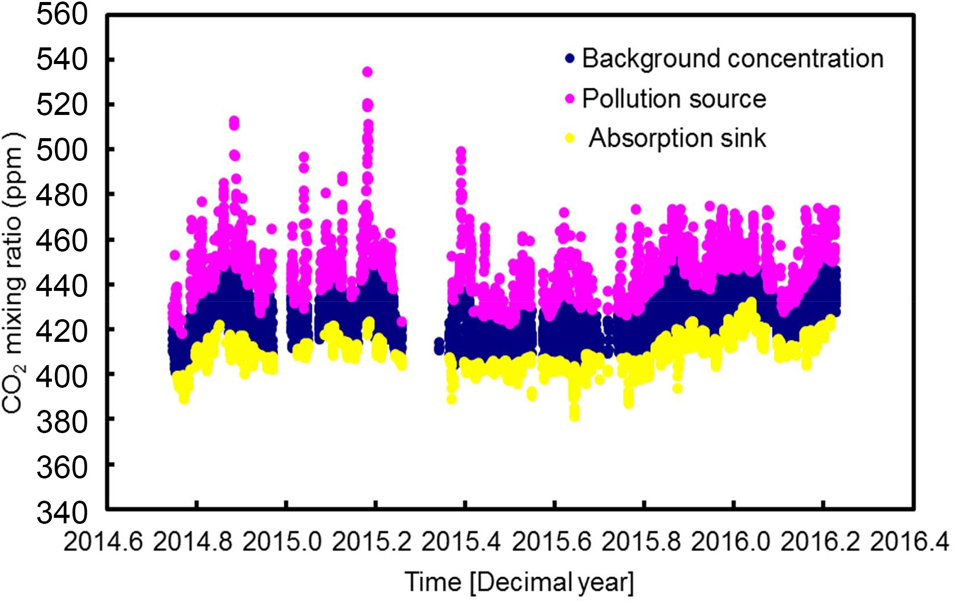
Figure4. Selected hourly XCO₂ data from GPACS from October 2014–March 2016.



2 -->

3.2. Temporal distribution of background CO₂ mole fractions

Figure 5a shows the seasonal distribution of diurnal background XCO₂ at GPACS. The XCO₂ was at a minimum from 1400–1600 LST, increased after 1700 LST, and reached a maximum at 0500 LST the next day. GPACS is located in the subtropical region, where variations of air temperature (yearly average: 26.71°C ± 6.11°C) and solar radiation are relatively small year round. The photosynthetic/respiration fluxes are active and the diurnal CO₂ variations are consequently obvious, which would thus decrease or elevate the overall background values. After sunrise the photosynthetic CO₂ uptake and air convection are enhanced, causing the CO₂ to decrease gradually and reach a minimum during the 1400–1600 LST time period. In the late evening, photosynthesis stops and respiration processes dominate, the boundary layer becomes neutral or stable, and a thermal inversion usually occurs, therefore contributing to increasing the background XCO₂ near the surface and resulting in a maximum at dawn. In spring and in winter, the diurnal XCO₂ was similar, and the difference was not significant (427.92 ± 2.26 ppm in winter, 426.58 ± 1.29 ppm in spring, p > 0.05). However, the reason was different. In winter, photosynthesis was the lowest, and the strong anthropogenic emissions can also increase the background XCO₂. By contrast, beginning from March in spring of the PRD region, photosynthesis becomes stronger. However, in spring, the PRD region typically experiences stagnant weather when the cold air suddenly becomes warm during the transition season between winter and spring (Zhang et al., 2014), which contributed to the XCO₂ accumulation. A distinct diurnal XCO₂ was observed in summer, in which the minimum value was lasting from 0900–1500. Such change was probably due to the meteorological conditions that favored the dispersion of XCO₂. The stronger photosynthesis at noon could also contribute to CO₂ uptake, resulting in overall lower background XCO₂. The peak-to-peak mean diurnal amplitudes were 12.63, 21.01, 15.02, and 10.25 ppm for spring, summer, autumn, and winter, respectively. The average magnitude of these amplitudes was lower than the results at Lin’an (LAN) station, but higher than those at LFS, Shangdianzi (SDZ), and WLG stations (Fang et al., 2014), reflecting the stronger solar radiation and complex local sources/sinks at GPACS. Figure 5b demonstrates the diurnal distribution of global solar radiation. The maximum value was observed in summer (487.26 ± 242.96 W m^?2), whilst it was moderate in autumn (392.74 ± 216.88 W m^?2) and lower in spring and winter (315.16 ± 239.78 and 290.04 ± 201.77 W m^?2, respectively). The variations of solar radiation in each season were similar to the amplitudes of diurnal XCO₂. This is because stronger solar radiation can enhance CO₂ uptake.
Figure5. Diurnal variation of background (a) CO₂ mole fractions and (b) global solar radiation in different seasons. Error bars represent standard deviations. The notches in the notched box and whisker plots present the 95% confidence levels of the median values. Non-overlapping notches indicate that the median values are significantly different from each other. MAM, March–April–May; JJA, June–July–August; SON, September–October–November; DJF, December–January–February.


Figure 6 shows the seasonal distribution of background XCO₂ in the PRD region. The value was highest in spring (427.99 ± 10.85 ppm) and winter (426.66 ± 8.55 ppm), moderate in autumn (423.71 ± 10.37 ppm), and lowest in summer (416.07 ± 6.80 ppm). The finding that the lowest XCO₂ levels occurred during the summer is consistent with the results from the global/regional stations of WLG, LFS, LAN, and SDZ (Fang et al., 2011). Given that the latitude of the PRD region is low, one possibility for the summertime minimum of CO₂ mole fractions is the flowering of vegetation, which results in the strongest photosynthesis of the year. Additionally, during the summer, the solar radiation is strong, and the stronger vertical convection and horizontal transport of the air facilitate the dilution of the XCO₂. It has been reported that the higher energy consumption of heating combined with the weakest photosynthesis of the year can result in the highest concentration of atmospheric CO₂ during the winter (Fang et al., 2011; Luan et al., 2014). In this study, the highest background XCO₂ did not occur in winter but rather in spring, which is consistent with the results at SDZ station (Fang et al., 2011). The PRD region typically experiences high-humidity weather in spring, when the ambient cold air suddenly warms during the transition from winter to spring (Zhang et al., 2014). Frequent airmass stagnation episodes in the spring season limit the diffusion of air pollutants, resulting in higher XCO₂ levels. Table 1 summarizes the background XCO₂ and its monthly fluctuations at GPACS, as well as at the global/regional background stations. Both the background XCO₂ and the monthly amplitude at GPACS were much higher than those at the global/regional background stations, indicating that the sources/sinks of CO₂ are complicated in the PRD region.

Season	CO2 mole fraction (ppm)
	GPACS	WLG*	LFS*	LA*	SDZ*
March–April–May	427.99	391.13	398.09	407.93	399.68
June–July–August	416.06	383.81	377.70	400.04	390.50
September–October–November	423.71	386.22	393.75	404.10	394.24
December–January–February	426.66	388.66	400.65	408.97	397.85
Monthly fluctuation	20.91	9.89	28.19	10.52	17.03
*Data from Fang et al. (2014).

Table1. Background CO₂ mole fractions and monthly fluctuations at GPACS and global/regional background stations.


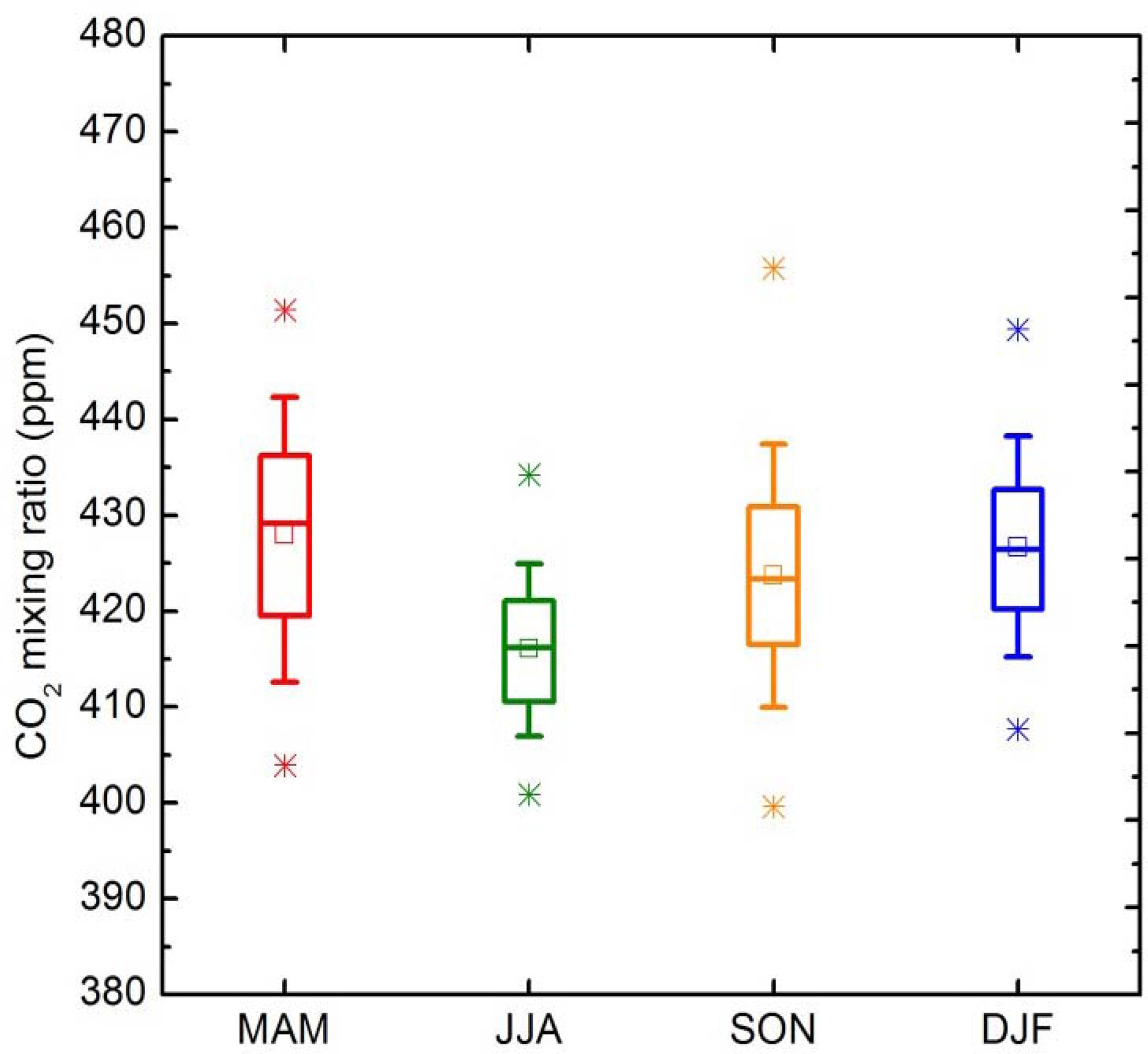Figure6. Seasonal distribution of the background mole fraction of CO₂ in the PRD region. The stars in the notched box and whisker plots represent maximum/minimum values, and the notches represent the 95% confidence levels of the median values. Non-overlapping notches indicate that the median values are significantly different from each other. MAM, March–April–May; JJA, June–July–August; SON, September–October–November; DJF, December–January–February.



2 -->

3.3. Cluster analysis

The 72-h backward trajectories were calculated from October 2014 to March 2016. The influence of the long-distance transport of polluted air masses on XCO₂ at GPACS was investigated using cluster analysis, which combines the trajectories into representative spatial groups using multivariate statistics to identify distinct transport patterns, with the angle distance (Ward’s minimum variance method) applied as the clustering criterion (Sirois and Bottenheim, 1995). Each trajectory in a cluster was used to obtain the cluster statistics (Zhang et al., 2013). There were 306, 310, 514, and 618 trajectories involved in the calculation of clusters for spring, summer, autumn, and winter, respectively.
Figure 7 shows the seasonal distributions of the isobaric trajectory clusters at GPACS. The trajectories during the spring, summer, autumn, and winter months were classified into six, five, five, and six clusters, respectively, indicating that the receptor was affected by complex air parcels. During the spring, cluster 2 and cluster 5 accounted for a large ratio, with a proportion of > 40%. The air parcels in these trajectories were mainly from southern Vietnam and the South China Sea. Cluster 1 and cluster 4 accounted for 19.9% and 16.9% of the trajectories, respectively. The proportion of cluster 3 and cluster 6 was less than 10%. During the summer, cluster 1 and cluster 3 contained more than 60% of the trajectories, and the airflows were similar to those of cluster 2 and cluster 5 during the spring. Cluster 2 from southeast of the PRD region accounted for 18.2% of the air parcels. Cluster 4 accounted for about 16.0% of the trajectories, in which the air masses were mainly from the conjunction region of Jiangxi and Hunan provinces. In autumn, cluster 3 and cluster 2 accounted for large ratios, with respective percentages of 39.0% and 34.3%. The air parcels in the former were typically from coastal areas east of Guangdong Province, while the air parcels in the latter were from the provinces of Anhui and Jiangxi. Cluster 4 was dominated by air masses from the Beibu Gulf and Qiongzhou Strait, accounting for 12.2% of the total trajectories. The cluster 1 proportion was 13.2% and represented air parcels from the PRD as well as the adjacent waters south of Taiwan. During the winter months, cluster 4 and cluster 5 accounted for a large percentage of nearly 36.5% of the total trajectories. Cluster 1 originated from the border area between Jiangxi and Hunan provinces, with a proportion of approximately 30.0%. Cluster 5, which contained air parcels passing through southern Guangxi Province and the west Guangdong region, accounted for 24.5% of the total trajectories. The air masses that passed over southern Taiwan and the Pearl River Estuary in cluster 3 accounted for about 20% of the total trajectories.
Figure7. Cluster analysis of 72-h back trajectories (500 m above the surface) in spring, summer, autumn, and winter at GPACS. The lines indicate clusters, numbers beside each cluster indicate the cluster sequence; the percentages represent the trajectory proportions of the total. MAM, March–April–May; JJA, June–July–August; SON, September–October–November; DJF, December–January–February.


In order to investigate the influences from regional sources on XCO₂, only the data representing the background and pollution were used in the cluster analysis. The values of 427.99 ppm, 416.06 ppm, 423.71 ppm, and 426.66 ppm, corresponding to the seasonal background means of XCO₂ in spring, summer, autumn, and winter (Fig. 4), were taken as threshold values when diagnosing whether a mole fraction was background or pollution. Table 2 shows the statistical CO₂ results of clusters in different seasons at GPACS. The polluted XCO₂ levels of the cluster air masses were 9.34–12.67 ppm higher than the corresponding background values, indicating that long-distance transport sources significantly influence XCO₂ at GPACS.

	Regional background					Pollution condition
	Cluster	Number of trajectories	CO2 mean value (ppm)	STD (ppm)		Number of trajectories	CO2 mean value (ppm)	STD (ppm)
MAM	1	39	433.6	6.97		44	440.29	8.31
	2	81	424.45	10.52		42	442.49	11.99
	3	15	434.21	7.79		14	438.24	6.69
	4	35	431.38	9.31		38	450.94	23.1
	5	19	421.21	10.19		16	446.21	17.52
	6	10	430.31	5.09		7	433.08	2.9
JJA	1	58	418.09	6.02		57	425.04	8.12
	2	41	418.13	5.46		45	426.82	8.49
	3	55	417.3	6.2		56	427.6	10.16
	4	32	415.2	6.89		25	429.31	12.43
	5	4	419.24	6.28		4	425.88	7.09
SON	1	52	427.14	8.36		45	438.21	13.12
	2	123	419.34	8.97		72	435.47	11.34
	3	110	426.27	9.66		120	441.06	13.46
	4	43	426.4	9.79		35	438.57	10.32
	5	3	426.68	2.73		4	433.67	14.15
DJF	1	127	424.56	7.8		76	437.15	8.37
	2	32	422.13	9.57		14	439.71	12.3
	3	70	426.97	9.32		72	443.39	11.96
	4	58	428.08	7.49		40	436.35	8.92
	5	103	428.85	7.3		99	439.24	10.03
	6	23	431.78	8.49		18	436.38	4.48
Notes: STD denotes one standard deviation; MAM, March–April–May; JJA, June–July–August; SON, September–October–November; DJF, December–January–February.

Table2. Statistical CO₂ results of clusters in different seasons at GPACS.


During the spring, cluster 4 exhibited an overall increase in XCO₂, with the standard deviation reaching its maximum. The air masses in this cluster may indicate a potential source region of CO₂ and reflect emissions from maritime transportation and fishing boats. Cluster 5 and cluster 2 represent air masses from southern Vietnam and the South China Sea, with relatively low mole fractions of CO₂ compared with those observed in cluster 4. During the summer, compared with the other seasons, the CO₂ mole fraction in each trajectory of clusters was much lower. The most elevated CO₂ mole fractions were associated with cluster 4, reflecting emissions associated with human activities from the border region between Jiangxi and Hunan provinces. Trajectories in cluster 2 and cluster 3 corresponded to moderate XCO₂. The former were from long-distance transport from the South China Sea, while the latter originated from southeast of the Pearl River Estuary, and may be associated with human activities (i.e., marine transportation, fishing boat engine emissions, and offshore oil exploitation). In autumn, the highest XCO₂ levels and the largest number of trajectories occurred in cluster 3, in which the airflows originated from the coastal areas of east Guangdong Province and thus may be a potential source of CO₂. The XCO₂ levels in cluster 5 and cluster 1 were equivalent. However, the latter exerts more influence on the background XCO₂ since it contains approximately 10 times the number of polluted trajectories than the former. Note that cluster 2 corresponds to lower XCO₂ mole fractions but accounts for the highest percentage of the total trajectories and thus has great influence on the XCO₂. During the winter season, the highest XCO₂ was found in cluster 3, whose trajectories originated from the southern waters of Taiwan and the Pearl River Estuary, and thus was a potential region of high XCO₂. Cluster 5 corresponds to air parcels passing through southern Guangxi Province and western Guangdong Province, where fossil fuel combustion dominates. Cluster 1 is associated with lower values of CO₂ mole fractions, in which the air masses were mainly affected by human activities from Hubei and Hunan provinces. This cluster contains the largest number of trajectories, and represents potential pollutant source regions from high latitudes.

2 -->

3.4. Probability distribution of the CO₂ potential source region

Figure 8 shows the probability density of XCO₂ in the source region during different seasons. In general, the CO₂ source locations identified by the WPSCF were very similar to the results obtained by the cluster method. In the spring season, the high WPSCF value region (from yellow to deep red, WPSCF > 0.5) spread from southeast to northwest and included three potential maxima. One of these is the region encompassing southeastern Taiwan, the southeast Pearl River Estuary, and the area south of the PRD region. Another is the region extending from the Qiongzhou Strait to the PRD region west of Guangdong Province, which is an area with a growing economy. In addition, a gradual increase in the WPSCF value can be observed from the provinces of Hubei and Hunan, with a maximum value occurring in the northern PRD region, indicating a band-shaped potential source region consisting of growing dense population centers and industry. During the summer season, photosynthesis strengthens, removing much of the CO₂ from the air. In addition, the higher temperatures also strengthen the upwelling CO₂ convection and horizontal diffusion. The WPSCF value expands generally from south to north, with the yellow to deep red region decreasing significantly. The high WPSCF summertime values mainly occurred in Hunan Province, and regions of northern Guangdong Province. In autumn, the potential CO₂ source regions were mainly concentrated in coastal areas of east Guangdong Province where the human emissions have the greatest impact. The second-highest WPSCF value region consisted primarily of the polluted areas of Hubei and Hunan provinces as well as northern Guangdong Province. The adjacent marine region south of Taiwan, the marine regions southeast of the Pearl River Estuary, and the Pearl River Estuary itself are identified mainly by yellow colors in Fig. 8, suggesting a potential CO₂ source of marine transportation, fishing boat engine emissions, and offshore oil exploitation. During the winter, the yellow to deep red regions extended from the PRD towards the west, north, and southeast, with three high WPSCF value centers distributed therein: (a) the first from the provinces of Hubei and Hunan to the PRD; (b) the second from Guangxi and western Guangdong to the PRD; and (c) the third distributed mainly in the marine regions southeast of the Pearl River Estuary and the PRD region. The above three centers covered the largest area during the winter, with the highest WPSCF values, indicating a high probability of strong CO₂ sources.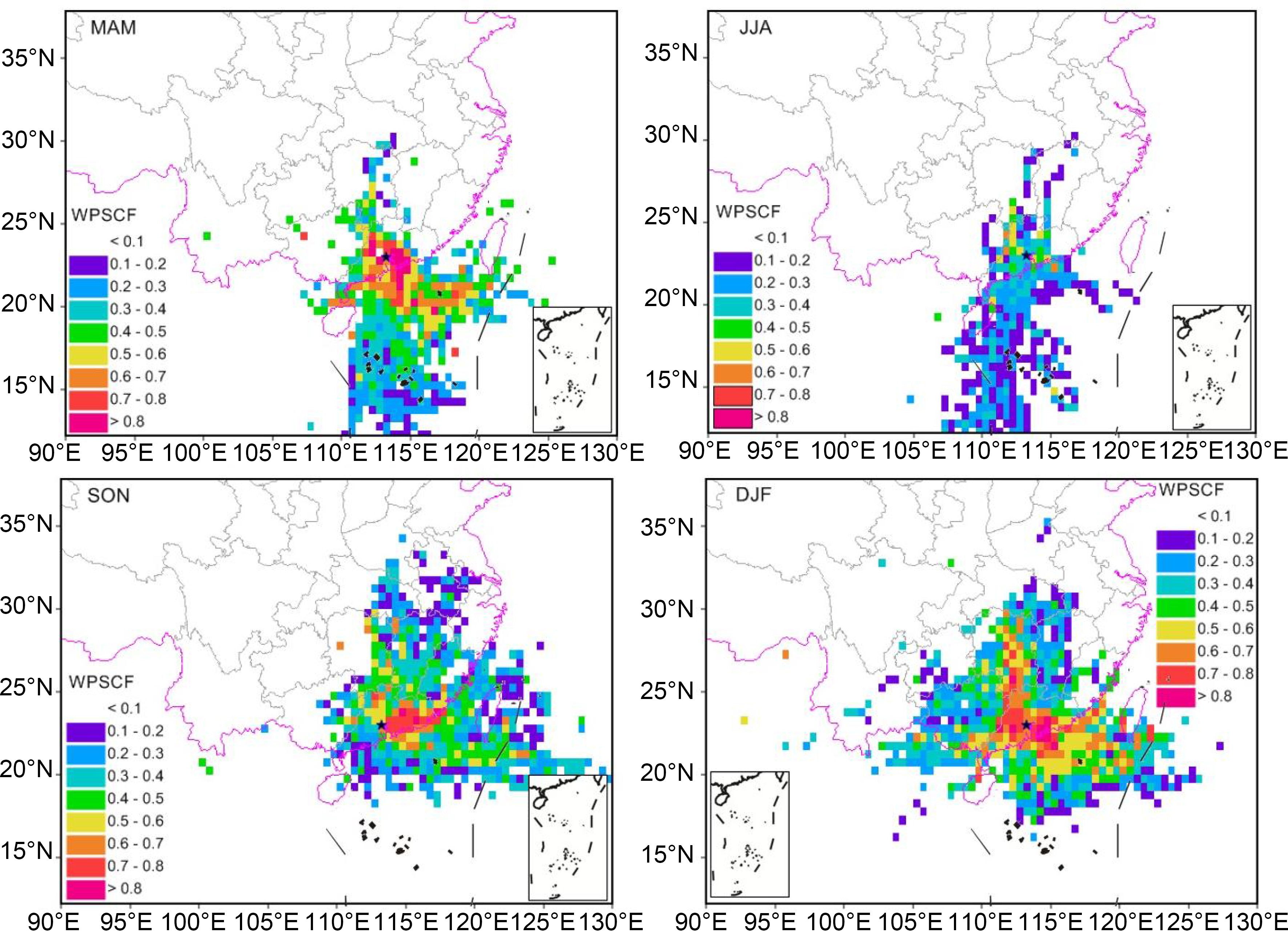
Figure8. Probability characteristics of the atmospheric CO₂ potential source region in different seasons. MAM, March–April–May; JJA, June–July–August; SON, September–October–November; DJF, December–January–February.


Throughout the year, the high WPSCF value regions were mainly distributed to the north of GPACS, mainly from Hunan and Hubei provinces to the PRD, indicating that human activities are the sources of high-latitude emissions. With the exception of summer, the south Taiwan Strait as well as southeast of the Pearl River Estuary were found to be strong potential source regions of CO₂, which is likely due to emissions from human activities in the maritime regions. The highest WPSCF value region was located in polluted areas from eastern Guangdong Province extending to the PRD, suggesting a strong potential source region.

Urban areas emit more CO₂ than forest ecosystems (Briber et al., 2013; Rosenzweig et al., 2010). However, studies involving the monitoring of anthropogenic greenhouse gas emissions in cities are scarce (Strong et al., 2011; Newman et al., 2012), especially in China. Most estimates of China’s energy-related carbon emissions are derived from official energy statistics, which are subject to large uncertainties (Wang et al., 2010). Monitoring of the CO₂ concentration in the urban areas contribute to the constraints that will reduce uncertainty in the bottom-up estimates of the Chinese carbon budget.
In this study, background/non-background XCO₂ and potential source regions were comprehensively investigated in the highly industrialized PRD region. Approximately 66.63%, 19.28%, and 14.09% of the observed values were filtered as background, pollutant source, and absorption sink data, respectively, through the application of a robust local regression mathematical method. Their corresponding mean values were found to be 424.12 ± 10.12 ppm, 447.83 ± 13.63 ppm, and 408.83 ± 7.75 ppm. All of the observed CO₂ exhibited larger fluctuations than those of the background CO₂, indicating that the CO₂ in the PRD region was strongly influenced by regional or local emission sources and absorption sinks.
The background XCO₂ in the PRD was highest in spring and winter, moderate in autumn, and lowest in summer. The diurnal value was at a minimum from 1400–1600 LST, reaching a maximum at 0500 LST the next day. The magnitude of peak to-peak mean diurnal amplitude was highest in summer and relatively low in the other seasons. The seasonal and diurnal variations of background XCO₂ were the results of air diffusion and thermodynamic transfer in the troposphere as well as the photosynthetic CO₂ uptake and respiration of vegetation.
The trajectories corresponding to the elevation of atmospheric XCO₂ in the PRD region exhibited significant seasonal variability. Throughout the year, air masses from the high-latitude regions of Hubei and Hunan provinces could lead to an overall elevation of XCO₂ in the PRD. The increase of XCO₂ during the spring and summer was primarily influenced by polluted air parcels from the southern Vietnamese waters, the South China Sea, and the area southeast of the Pearl River Estuary. With the exception of summer, the airflow patterns primarily from southeastern Taiwan passing over the Pearl River Estuary exerted greater impacts on XCO₂, suggesting an important potential source region.
Acknowledgements. This research work was funded by the National Key R&D Program of China (Grant No. 2018YFC0213902, 2019YFC0214605, 2016YFC0202000), the open project of the Key Laboratory for Aerosol-Cloud-Precipitation of China Meteorological Administration, Nanjing University of Information Science and Technology (KDW 1803), the Scientific and Technological Innovation Team Project of Guangzhou Joint Research Center of Atmospheric Sciences, China Meteorological Administration (Grant No.201704), the Science and Technology Research Project of Guangdong Meteorological Bureau (Grant No. GRMC2018M01). The availability of the data used in this study is fully described in section 2 of this paper. The authors thank the developers of the HYSPLIT-4. Constructive suggestions from Dr. Timothy LOGAN, as well as from the anonymous reviewers, are greatly appreciated.