HTML
--> --> -->Various stochastic physics schemes have been developed and implemented to represent model uncertainties in different EPSs (Bowler et al., 2008; Berner et al., 2009; Palmer, 2012; Yuan et al., 2016). The stochastically perturbed parameterization tendencies (SPPT) scheme, which represents model uncertainties by stochastically perturbing the net physics tendencies (Palmer et al., 2009), improves the probability forecast skill and requires fewer resources to maintain (Leutbecher et al., 2017). The stochastic kinetic energy backscatter (SKEB) scheme, in which a fraction of the dissipated energy is backscattered upscale and acts as a streamfunction forcing for the resolved-scale flow (Shutts and Palmer, 2004, Shutts, 2005, Berner et al. 2009), represents model uncertainties by stochastically perturbing the stream function (Shutts, 2005) and accounts for the improvement in spread within the ensemble system (Berner et al., 2009). A drawback of both the SPPT and SKEB schemes is that they do not respect the energy conservation rule, which leads to inconsistencies. Perturbations are not introduced into the fluxes at the surface and at the top of the atmosphere, resulting in an energy imbalance and individual ensemble members no longer conserve energy (Ollinaho et al., 2017). While deterministic models themselves are not always fully conservative, SPPT and SKEB may exacerbate this to an unwanted extent, and thus there is a need to see if dramatic changes to energy take place when introducing these stochastic schemes into the ensemble system.
Another stochastic method for representing model uncertainties is to add stochastic perturbations to uncertain parameters within the physics parameterization schemes. Parameter uncertainties mainly derive from the inaccurate estimation of parameters by empirical, semi-empirical, observational or statistical methods. It is challenging to give these parameters a precise deterministic value because they vary with the atmospheric conditions and underlying surface environment. Different EPSs adopt different approaches to represent the large uncertainties in parameters within physical parameterization schemes. For example, since 2008, the UK Meteorological Office has used a random parameter scheme that introduces perturbations that only vary in time (Bowler et al., 2008). Christensen et al. (2015) used informed parameter covariances to perturb four convection closure parameters within the European Centre for Medium-Range Weather Forecasts (ECMWF) Integrated Forecasting System.
A newly developed method, different from the methods mentioned above, is the stochastically perturbed parameterization (SPP) scheme (Ollinaho et al., 2017). In this study, the SPP scheme in the Global and Regional Assimilation and Prediction Enhanced System—Regional Ensemble Prediction System (GRAPES-REPS) (Xu et al., 2019) is applied to consider possible sources of uncertainties. SPP introduces temporally and spatially varying perturbations at each time step to key parameters within the parameterization schemes, and temporal and spatial correlations are obtained through a first-order auto-regressive process (Li et al., 2008; Berner et al., 2009). An advantage of SPP over SPPT and SKEB is that it represents model uncertainties in a physically consistent way and can introduce perturbations into the surface and the top of the atmosphere while conserving the local energy budget (Leutbecher et al., 2017; Ollinaho et al., 2017). The implementation of SPP at the ECMWF is described in detail by Ollinaho et al. (2017).
There are many different sources of model error and it is challenging to characterize these errors completely and accurately with one single stochastic perturbation scheme (Leutbecher et al., 2017). Some operational national weather prediction centers have applied a combined approach—for example, Environment Canada (Charron et al., 2010) and the ECMWF (Palmer et al., 2009) combine SKEB and SPPT, whereas the UK Meteorological Office EPS (or MOGREPS) uses a random parameter scheme together with the SKEB scheme (Berner et al., 2009) to give an improved forecast skill. The National Oceanic and Atmospheric Administration (NOAA) combined SPP, SPPT, and SKEB (Jankov et al., 2017) and found that the ensemble combining three stochastic schemes consistently produces the best spread–skill ratio and generally outperforms the multiphysics ensemble. This suggests that a combination of different stochastic physics schemes might have the potential to better deal with the model uncertainties.
With the aim of representing model uncertainties more comprehensively, we combined the SPP, SPPT, and SKEB schemes to form different combinations for the first time over China, to take the possible sources of uncertainties into account for long-term evaluation. Compared with other regions of the world, China is a well-documented monsoon region with a unique monsoon climate and complex topography and landscape (e.g., the Tibetan Plateau) (Flohn, 1957). Therefore, the sources and growth of forecast error in the monsoon region are generally complicated, and thus how to represent the forecast error of the monsoon region and construct a reasonable model perturbation technique is a problem worthy of further study. In GRAPES-REPS, the SKEB scheme represents the model uncertainties arising from energy dissipation by stochastically perturbing the stream function. The SPPT scheme perturbs the total parameterization tendencies, which include those from all parameterizations in GRAPES (i.e., microphysics, cumulus convection, radiation, boundary layer, land surface, gravity wave drag parameterization schemes) to address the uncertainties associated with the physics parameterizations (Yuan et al., 2016). The SPP scheme targets uncertainties at their sources within the parameterization schemes and links with individual physical processes. A similar experiment was conducted by Jankov et al. (2017) in an ensemble based on Rapid Refresh. In their SPP implementation, they perturbed four uncertain parameters in convective and boundary layer parameterization schemes and applied the same temporal and spatial decorrelations of stochastic patterns to perturb the parameters in SPP as those in SPPT [also see Christensen et al. (2015)].
We have implemented a comprehensive SPP scheme in GRPAES-REPS (Xu et al., 2019). This SPP scheme perturbs more uncertain parameters (i.e., 18 parameters) to account for the uncertainties in four physics parameterization schemes: the convection, boundary layer, surface layer, and microphysics parameterizations. Perturbing more uncertain parameters contributes to an increase in the random variability and a greater number of parameter values can be reached and explored during the forecast period. In addition, the temporal and spatial decorrelations of the stochastic pattern used to perturb the parameters in SPP are different from those in SPPT; we believe these should be set differently in the two methods. The SPP scheme should be developed to measure the temporal and spatial decorrelation scales of the perturbations and to improve the forecast skill. We carried out sensitivity experiments on temporal and spatial decorrelations and their standard deviations.
This paper is organized as follows. The configurations of GRAPES-REPS and the experimental design are described in section 2. A detailed description of the three stochastic physics schemes is provided in section 3. Section 4 presents the results of both the precipitation verification and surface and upper-air verification. An analysis of the kinetic energy (KE) spectrum and the added value of SPP are addressed in sections 5 and 6. A summary and discussion are given in section 7.
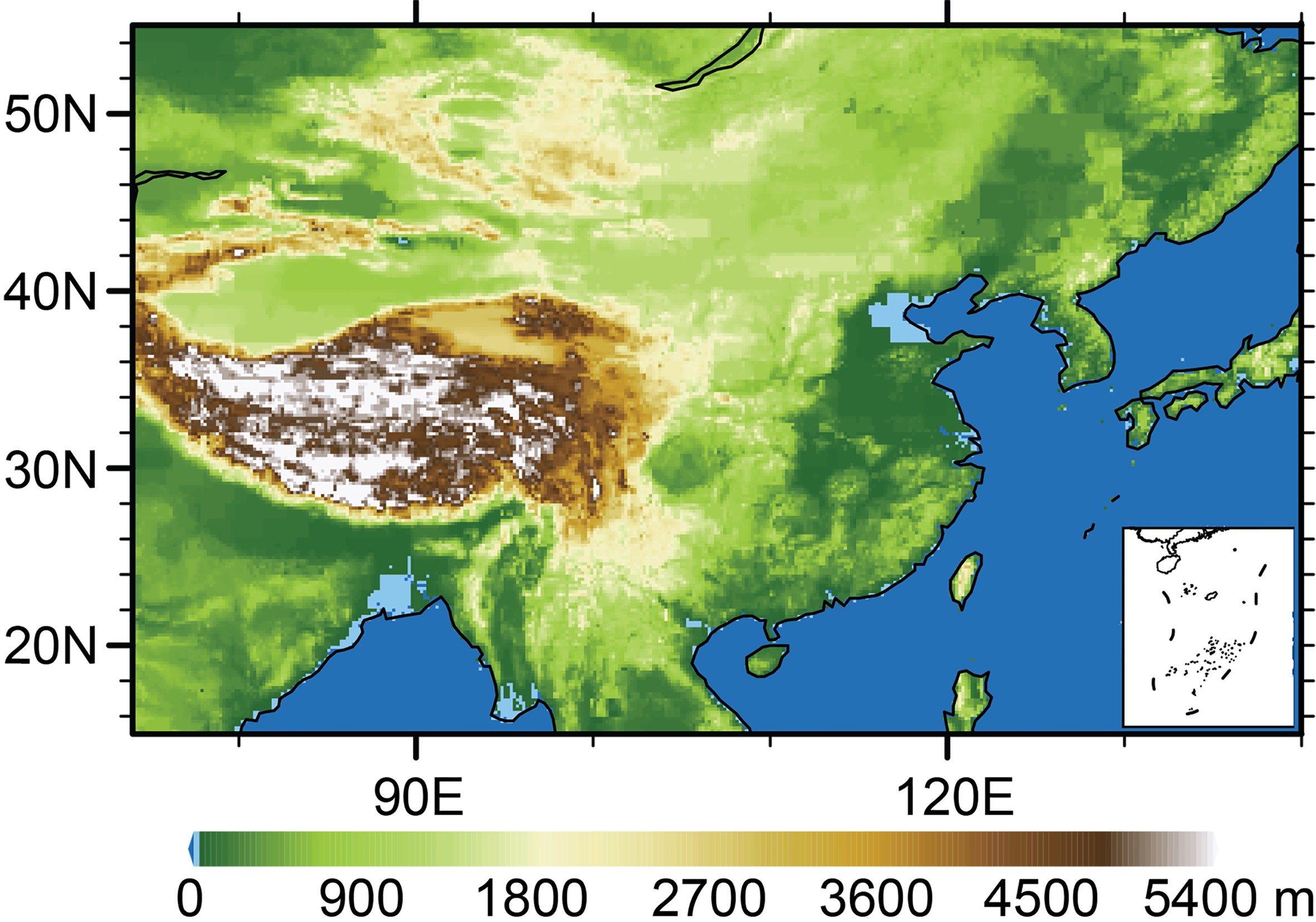 Figure1. Domain and topography for the model simulation.
We applied the SPP, SPPT, and SKEB schemes to develop and evaluate different combinations of multiple stochastic physics schemes. Five stochastic experiments and one control (CTL) experiment were conducted in GRAPES-REPS (Table 1) for a summer month (1–30 June 2015) over China. Different combinations of stochastic physics schemes represent different aspects of the model uncertainties.
| Experiment | Initial condition | Physical perturbation method |
| CTL | Downscaling | None |
| SPP | Downscaling | SPP |
| SPP_SPPT | Downscaling | SPP, SPPT |
| SPP_SKEB | Downscaling | SPP, SKEB |
| SPPT_SKEB | Downscaling | SPPT, SKEB |
| SPP_SPPT_SKEB | Downscaling | SPP, SPPT, SKEB |
Table1. Experiments conducted in this study.
3.1. SPP scheme
33.1.1. Parameter selection
We selected the 18 key parameters that may have a significant impact on precipitation from the Kain–Fritsch convection (Kain and Fritsch, 1990; Kain, 2004), Medium-Range Forecast Planetary Boundary Layer (MRF-PBL) (Hong and Pan, 1996) and WRF Single-Moment 6-class (WSM6) microphysics (Hong and Lim, 2006) and Monin–Obukhov (Beljaars, 1995) surface layer parameterization schemes. Descriptions and ranges of the parameters selected are presented in Table 2.| Parameter | Scheme | Default | Range | Description |
| BRCR | MRF | 0.5 | [0.25, 0.75] | Critical Richardson number |
| PFAC | MRF | 2.0 | [1, 3] | Profile shape exponent for calculating the momentum diffusivity coefficient |
| KARMAN | MRF | 0.4 | [0.38, 0.42] | Von-Kármán constant |
| CFAC | MRF | 7.8 | [3.9, 15.6] | Coefficient for Prandtl number |
| XKA | Monin–Obukhov | 2.4×10?5 | [1.2×10?5, 5.0×10?5] | The multiplier for heat/moisture exchange coefficient |
| CZO | Monin–Obukhov | 0.0156 | [0.01, 0.026] | The Charnock parameter |
| EACRC | WSM6 | 1.0 | [0.6, 1] | Snow/cloud-water collection efficiency |
| DENG | WSM6 | 500 | [300, 700] | Density of graupel (kg m?3) |
| XNCR | WSM6 | 3.0×10⁸ | [1.0×10⁷, 1.0×10⁹] | Maritime cloud content (%) |
| N0R | WSM6 | 8.0×10⁶ | [5.0×10⁶, 1.2×10⁷] | The intercept parameter of rain (m?4) |
| PEAUT | WSM6 | 0.55 | [0.35, 0.85] | Collection efficiency for cloud water converting to rain (g/g.s) |
| DIMAX | WSM6 | 5.0×10?4 | [3.0×10?4, 8.0×10?4] | The limited maximum value for the cloud-ice diameter (m) |
| PD | Kain–Fritsch | 1.0 | [0.5, 2] | The multiplier for downdraft mass flux rate |
| PE | Kain–Fritsch | 1.0 | [0.5, 2] | The multiplier for entrainment mass flux rate |
| PH | Kain–Fritsch | 150 | [50, 350] | The starting height of downdraft above updraft source layer (hPa) |
| TIMEC | Kain–Fritsch | 2400 | [1800, 3600] | Average consumption time of convective available potential energy (s) |
| W0 | Kain–Fritsch | 0.75 | [0.04, 0.1] | The threshold vertical velocity in the trigger function (m s?1) |
| TKEMAX | Kain–Fritsch | 5.0 | [3, 12] | The maximum TKE value in sub-cloud layer (m2 s?2) |
Table2. The parameters selected in this paper. The identifier of parameters and the scheme that the parameters are in are presented in the first and the second column, respectively. The default values of the parameters are given in the third column, and the fourth column indicates the realistic empirical ranges of the parameters. Finally, definitions of the parameters are provided in the last column.
In the following we briefly explain the motivation for selecting the above parameters. The parameters and their ranges were determined based on the literature (e.g., ECMWF IFS Documentation Part IV: P HYSICAL PROCESSES (CY25R1), 2003; Reynolds et al., 2011; Baker et al., 2014; Johannesson et al., 2014; Di et al., 2015; Mccabe et al., 2016), and following the parameter sensitivity analysis work of Di et al. (2015), Baker et al. (2014) and Johannesson et al. (2014) and consultations with GRAPES physics parameterization experts (J. CHEN, G. XU, Q. LIU, personal communication, 2017).
In the boundary layer parameterization scheme, boundary layer height is defined as the level where the bulk Richardson number reaches the critical value of Richardson number (BRCR) (ECMWF IFS Documentation Part IV: P HYSICAL PROCESSES (CY25R1), 1–174). Furthermore, Hong and Pan (1996) found that convective precipitation is particularly sensitive to the critical Richardson number (BRCR). In addition, the profile shape exponent for calculating the momentum diffusivity coefficient (PFAC) is highly sensitive in the simulation of precipitation because it directly affects the development of convection in the boundary layer (Di et al., 2015). The Von-Kármán constant (KARMAN), which is a constant of the logarithmic wind profile in the surface layer, and the CFAC, which is a coefficient for the Prandtl number at the top of the surface layer, were both closely related to characteristics of momentum, heat, and mass transfer (Reynolds et al., 2011; Di et al., 2015). These parameters were therefore selected for the boundary layer parameterization scheme.
In the surface layer parameterization scheme, Zhang and Anthes (1982) found that the structure of the PBL is highly sensitive to the roughness length. The roughness length is therefore indirectly perturbed through the Charnock parameter (CZO), which determines the magnitude of the wind-speed-dependent roughness length over the oceans and was also selected in the random parameter scheme (Baker et al., 2014). The multiplier for the heat/moisture exchange coefficient (XKA) is both sensitive and significant, as the XKA value predominantly reveals the strength of the flux exchange (Di et al., 2015). The parameters CZO and XKA were therefore selected in the surface layer parameterization scheme.
In the convection parameterization scheme, the most significant and sensitive parameters are the downdraft and entrainment mass flux rates, which represent mixing of the cloud with the environment (Kain, 2004). Yang et al. (2012) and Di et al. (2015) indicated that PD and PE, which are the multipliers for the downdraft and entrainment mass flux rates, respectively, are closely related to the downdraft and entrainment mass flux rates and physically affect the convective process. The starting height of the downdraft above the updraft source layer (PH), which controls the structure of the downdraft, has a significant effect on the convection process (Di et al., 2015). In addition, the mean consumption time of the convective available potential energy (TIMEC) efficiently controls the development of convection and has a considerable impact on convective precipitation (Johannesson et al., 2014; Di et al., 2015). The threshold vertical velocity (W0) in the trigger function is highly sensitive (Kain, 2004; Li et al., 2008) and can be stochastically perturbed for ensemble forecasts (Bright and Mullen, 2002). The intensity of updraft mass flux at the updraft source layer is assumed to be a function of turbulent kinetic energy (TKE) for shallow convection and the maximum turbulent kinetic energy (TKEMAX) has been proven to be significant for convective precipitation (Yang et al., 2012; Di et al., 2015). The parameters PD, PE, PH, TIMEC, W0, and TKEMAX were therefore selected in the convection parameterization scheme.
In the microphysics parameterization scheme, the properties of the scheme are sensitive to the size distribution of ice particles and therefore the intercept parameter (N0R), which directly influences the distribution of the entire range of drop sizes in the exponential distribution of raindrop size, was selected (Hacker et al., 2011; Di et al., 2015). Jiang et al. (2010) and Baker et al. (2014) confirmed the significance for precipitation of the collection efficiency for the conversion of cloud water to rain (PEAUT) and the limited maximum value for the diameter of cloud ice (DIMAX) because these parameters affect the conversion of clouds to rain. Three other uncertain parameters—the snow/cloud water collection efficiency (EACRC), the density of graupel (DENG) and the maritime cloud content (XNCR)—are also selected based on the results of Johannesson et al. (2014) and the suggestions of experts. First, the snow-/cloud-water collection efficiency (EACRC), which represents the ratio of cloud coagulation, and the coagulation between large and small cloud droplets can convert cloud droplets into precipitation, so there is a direct impact on precipitation; second, the density of graupel (DENG), which greatly influences the precipitation efficiency and thereby represents a part of the uncertainty in the heavy rainfall process, is also perturbed; and third, the maritime cloud content (XNCR), which is a multiplier for the automatic conversion rate, is the direct factor of influence in the transformation of cloud water to rain water and thereby has an important effect on precipitation. The parameters N0R, PEAUT, DIMAX, EACRC, DENG, and XNCR were therefore selected in the microphysics scheme.
3
3.1.2. Design of the SPP scheme
The parameters in the SPP scheme are perturbed stochastically and vary within a reasonable range set within the realistic empirically tuned value of each parameter. Temporal and spatial correlations are obtained through a first-order auto-regressive process (Li et al., 2008; Berner et al., 2009). A lognormal distribution (Ollinaho et al., 2017) is used to describe the distribution of the perturbed parameters:The perturbed and unperturbed parameters are referred to as ξj and


where the variables λj, ?j and tj are longitude, latitude and time, respectively. The


where


where


The probability density function distribution of the random field


Note that the different parameters have independent stochastic patterns because they use different random seeds to generate the random number used to initiate the Markov process. The perturbation pattern


 Figure2. The perturbation pattern
The SPP scheme in this study uses the same random field generator as the SPPT scheme, but with larger scale correlation patterns (a spatial correlation scale of L = 20 and a temporal correlation scale of τ = 12 h). We conducted sensitivity experiments on the temporal and spatial decorrelations and standard deviations in GRAPES-REPS and the best results were achieved when choosing spatial decorrelations of L = 20 (i.e., each wave spans approximately 375 km in the latitude over the verified domain), temporal decorrelations of τ = 12 h and standard deviations of σ = 0.8 (Xu et al., 2019). The results indicate that larger perturbation patterns show better skill, which is also argued by Ollinaho et al. (2017). This may be explained by the fact that if the parameter perturbations vary too quickly, then it may be difficult to observe and measure their significant impact. If the parameters vary more slowly, then the perturbations have more time to affect the critical areas of the developing weather phenomenon and therefore a larger impact is observed and measured during the period of the forecast.
The perturbed parameters are confined within strictly specified bounds (between ξmax
2
3.2. SPPT scheme in GRAPES-REPS
The SPPT scheme in GRAPE-REPS represents the structural uncertainties associated with the physics parameterizations by perturbing the net tendencies with noise correlated in space and time (Yuan et al., 2016). The net tendency term is referred to as X and
The random field


| SPP | SPPT | SKEB | |
| Temporal correlation scale τ | 12 h | 6 h | 6 h |
| Spatial correlation scale L | 20 | 24 | [50, 100] |
| Standard deviation σ | 0.8 | 0.27 | 0.27 |
| Specified bounds | Varying with parameters | [0.2, 1.8] | [?0.8, 0.8] |
| Mean of the random field μ? | 0.0 | 1.0 | 0.0 |
| Constant β | ?1.27 | ?1.27 | ?1.27 |
Table3. Stochastic perturbation parameter options for SPP, SPPT, and SKEB.
2
3.3. SKEB scheme in GRAPES-REPS
The SKEB scheme represents the model uncertainty derived from the dissipation of energy by stochastically perturbing the stream function. In the SKEB scheme, the fraction of the dissipated energy that acts as streamfunction forcing for the resolved-scale flow is backscattered upscale in the physical parameterization processes.The horizontal wind is perturbed stochastically (note that temperature is not perturbed in this study) according to
where su and sv are small-scale forcing terms:
Following Shutts (2005), Fψ is given by:
The random field


In verification of surface and upper-air weather variables, weather variables such as the 250-hPa zonal wind speed, 500-hPa temperature, 850-hPa zonal wind speed and temperature, 10-m zonal wind speed, and 2-m temperature, are assessed to verify the forecasts. The verification results for the zonal (U) and meridional (V) wind speed are similar, so only the former (U) is presented here. The zonal wind speed at 250 hPa is important when considering convection because deep convection stops and convective outflow generally occurs at the tropopause (around 250 hPa in summer) and this phenomenon can be detected in the 250-hPa zonal wind (Christensen et al., 2015). The temperature and zonal wind speed at 850 hPa are assessed because 850 hPa corresponds to the top of the boundary layer for areas near sea level (about 1.5 km). Near-surface variables, 10-m zonal wind speed and 2-m temperature, are also considered. The verification metrics used in surface and upper-air verification are the root-mean-square error (RMSE), the ensemble spread, consistency (defined as the ratio of the spread to the RMSE), the continuous ranked probability score (CRPS; Hersbach, 2000), Talagrand diagrams (Talagrand et al., 1997), and the outlier score. Brief definitions of these metrics are presented here and more detailed information is given in Jolliffe and Stephenson (2003).
An Unpaired Student’s t-test in which we reject a null hypothesis at the 0.05 level of significance is performed to test the significance of the results—the null hypothesis being that the differences between the time-averaged reference CTL experiment and the time-averaged SPP, SPP_SPPT, SPP_SKEB, SPPT_SKEB, and SPPT_SPP_SKEB experiment are zero.
The background data for GRAPES-REPS are obtained by dynamical downscaling of the T639 [T639 global medium-term numerical forecast system (Guan et al., 2008)] ensemble forecast background data. The forecasts of surface and upper-air weather variables are verified against the GRAPES 15 km gridded analysis from the National Meteorological Information Center (Chen et al., 2006).
2
4.1. Precipitation verification
The precipitation forecasts are verified by first evaluating the probabilities of precipitation exceeding specific thresholds, and then calculating the AROC score [which measures the statistical discrimination capability of an EPS (Mason, 1982)]. The frequency bias, which is the ratio of the frequency of forecast occurrence and the frequency of observations (Schaefer, 1990), is used as a measure of deterministic performance.Before conducting the statistical analysis, probabilities of precipitation exceeding the 25-mm (Figs. 3a, c, e, g, i, k) and 50-mm (Figs. 3b, d, f, h, j, l) thresholds for monthly mean 24-h accumulated precipitation of the CTL experiment (Figs. 3a, b), SPP minus CTL experiment (Figs. 3c, d), SPP_SPPT minus CTL experiment (Figs. 3e, f), SPP_SKEB minus CTL experiment (Figs. 3g, h), SPPT_SKEB minus CTL experiment (Figs. 3i, j), and SPP_SPPT_SKEB minus CTL experiment (Figs. 3k, l) are evaluated. As shown in the probability difference plots (Figs. 3c–k), for both the 25- and 50-mm thresholds, all the stochastic experiments are characterized by higher probabilities (positive probability difference) than the CTL experiment in most of the precipitation regions, indicating that all the stochastic experiments can generally improve the ability of precipitation simulation. Moreover, the SPP_SPPT minus CTL experiment (Figs. 3e, f) generally performs better than the SPP_SKEB minus CTL experiment (Figs. 3g, h), which may indicate a greater impact of the SPPT scheme on simulated precipitation than the SKEB scheme. In general, the SPP_SPPT_SKEB minus CTL experiment (Figs. 3k, l) is characterized by the largest probability difference in the key precipitation region of the Bay of Bengal and South China, indicating that combining all three stochastic schemes (SPP, SPPT, and SKEB) can better simulate the probability distribution of precipitation, and provides better guidance in precipitation forecasts compared to other experiments. Also, the improvements seen with the CTL experiment and the SPP, SPP_SPPT, SPP_SKEB, SPPT_SKEB, and SPPT_SPP_SKEB experiment are statistically significant at the 98%, 99%, 95%, 98%, and 99.5% levels (t-test), respectively.
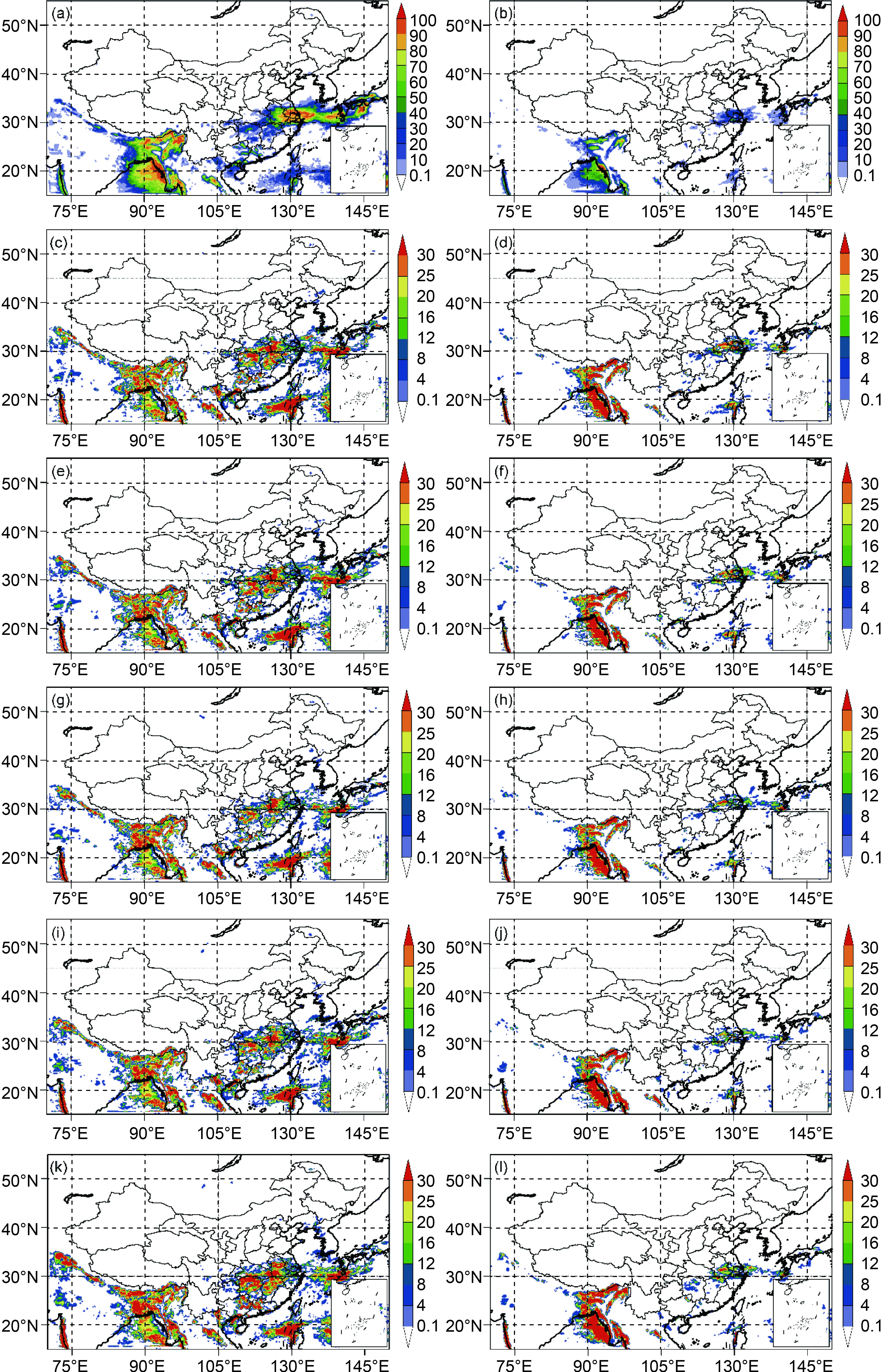 Figure3. Probability of precipitation exceeding (a, c, e, g, i, k) 25-mm and (b, d, f, h, j, l) 50-mm thresholds for monthly mean 24-h accumulated precipitation for the (a, b) CTL experiment, (c, d) SPP minus CTL experiment, (e, f) SPP_SPPT minus CTL experiment, (g, h) SPP_SKEB minus CTL experiment, (i, j) SPPT_SKEB minus CTL experiment, and (k, l) SPP_SPPT_SKEB minus CTL experiment. The results are the monthly averages for the 0000 UTC cycle during June 2015.
The AROC score, which represents the area between the ROC curve and the no-discrimination line, and measures the statistical discrimination capability of an EPS, is a commonly used metric for verification of probabilistic precipitation forecasts (Mason, 1982). It has a range of 0 to 1, where a score of 1 is attained for a perfect forecast and a score of 0 indicates no skill. Figures 4a–d show the AROC scores of the 24-h accumulated precipitation for the 0.1-, 10-, 25- and 50-mm thresholds, respectively. The ideal AROC score is 1.0. As shown in Fig. 4, all the stochastic experiments are characterized by higher AROC scores than the CTL experiment for all thresholds and forecast lead times, indicating that stochastic methods can effectively improve the probabilistic forecasting skill for precipitation. For light and moderate rain (Figs. 4a, b), the SPP_SPPT_SKEB and SPPT_SKEB experiments achieve higher AROC scores, whereas the SPP_SPPT_SKEB, SPP, and SPP_SPPT experiments perform better for heavier precipitation (Figs. 4c, d). The SPP_SPPT_SKEB experiment achieves the highest AROC scores for most of the thresholds and lead times, indicating that a combination of multiple schemes may better capture the uncertainties inherent in precipitation and increase the overall probability forecast skill. The difference in AROC scores between the CTL and the SPP_SPPT_SKEB experiments is statistically significant at the 99% level (t-test) for all thresholds at most of the lead times.
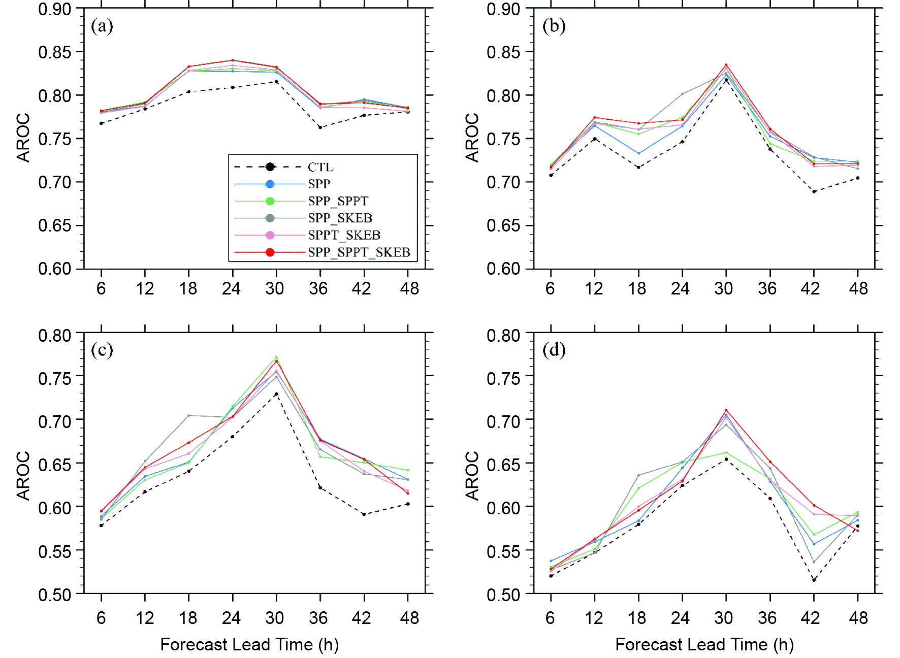 Figure4. The domain-averaged AROC scores of 24-h accumulated precipitation for four thresholds [(a) 0.1, (b) 10, (c) 25, (d) 50 mm] for the six experiments, varying with forecast hour. The results are the monthly average for the 0000 UTC cycle during June 2015.
Figure 5 evaluates the ensemble mean frequency bias, which measures the ratio of the frequency of forecast events to the frequency of observed events and indicates whether the forecast system tends to underforecast (frequency bias < 1) or overforecast (frequency bias > 1) events (Schaefer, 1990). The perfect value of 1.0 is ideal. As shown in Fig. 5, almost all stochastic experiments perform better than the CTL experiment, which implies an improvement for precipitation forecasting, and the SPP_SPPT_SKEB, SPP_SPPT, and SPP_SKEB experiments give a better representation of the amount of rainfall (the value of the frequency bias is closer to 1.0) for most of the forecast lead times and thresholds. The SPP_SPPT_SKEB and SPP_SPPT experiments perform well, especially for heavier precipitation (threshold > 25mm); that is, they better represent medium to heavy rainfall events. In addition, SPP has a higher frequency bias than all other experiments for the two lighter thresholds (Figs. 5a, b), which represents a relatively worse performance for the SPP experiment than other experiments, and this may due to the reason that perturbing parameters alone in the SPP experiment may not be a good representation of lighter thresholds. The difference in frequency bias between the CTL and the SPP_SPPT_SKEB experiments is statistically significant at the 99% level (t-test) for most of the thresholds at most of the lead times. Also, the improvements seen with SPP_SPPT_SKEB and SPP_SPPT are statistically significant at the 95%, 98%, 99% and 99.5% level (t-test) for the 12-, 18-, 24- and 30-h forecast lead times, respectively, for the 25-mm threshold. However, for the 50-mm threshold, the difference between the two is statistically significant at the 99% and 95% level only for the 30- and 42-h forecast lead times.
 Figure5. The ensemble mean frequency bias of 24-h accumulated precipitation for the six experiments for four thresholds [(a) 0.1, (b) 10, (c) 25, (d) 50 mm] varying with forecast hour. The results are the monthly average for the 0000 UTC cycle during June 2015.
2
4.2. Surface and upper-air verification
The horizontal distributions of the ensemble spread and RMSE for the CTL, SPP, SPP_SPPT, SPP_SKEB, SPPT_SKEB and SPP_SPPT_SKEB experiments are evaluated. Figures 6a–l compare the horizontal distributions of the ensemble spread and the RMSE of the ensemble mean for the 850-hPa wind speed for six experiments at a lead time of 48 h. Note that the results for the 250- and 500-hPa wind speed are similar to those of 850-hPa wind speed, and thus are not shown here. As shown in Figs. 6a and b, it can be clearly seen that the CTL experiment is underdispersive (i.e., too little spread compared to RMSE). The SPP (Fig. 6c) and SPP_SPPT (Fig. 6e) experiments produce a slight improvement of ensemble spread relative to the CTL experiment, and their distributions of spread are quite similar, implying a limited impact of SPPT on improving the ensemble spread. Combining the SKEB with the SPP and/or SPPT, SPP_SKEB (Fig. 6g), SPPT_SKEB (Fig. 6i) and SPP_SPPT_SKEB (Fig. 6k) experiments results in a notable increase in spread, which is clearly larger than that of the experiments without SKEB, and a similar RMSE is maintained over almost all the domain. SKEB directly perturbs the wind field and therefore its addition will greatly impact the upper-air wind-speed fields, and it contributes most to the improvement in spread for wind, while the addition of SPPT is not as dramatic. In addition, the improvement in spread for temperature is not as dramatic as that for the winds. The horizontal distribution of the ensemble spread for the temperature (not shown) has a similar distribution of spread for all experiments, which may be due to the reason that the SKEB scheme, which only acts on the wind field and does not affect the temperature field, contributes most to the improvement in spread. Note that such horizontal distributions of ensemble spread and RMSE for surface variables (e.g., 2-m temperature, 10-m wind speed; not shown here) are not as sensitive to SKEB as upper-air wind speeds because of the nature of the perturbations being applied.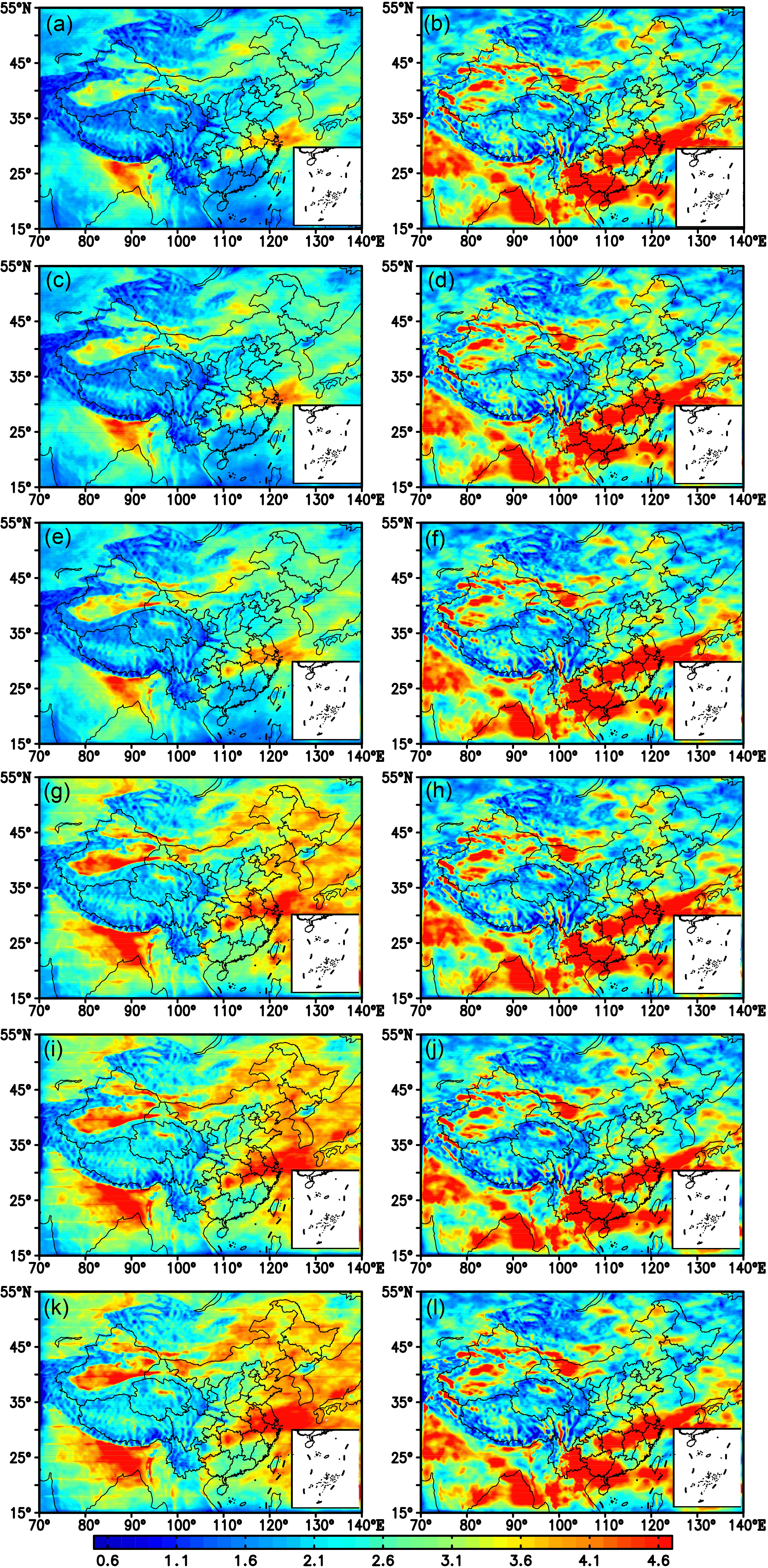 Figure6. The horizontal distribution of (a, c, e, g, i, k) ensemble spread and (b, d, f, h, j, l) RMSE of the ensemble mean for (a, b) CTL, (c, d) SPP, (e, f) SPP_SPPT, (g, h) SPP_SKEB, (i, j) SPPT_SKEB, and (k, l) SPP_SPPT_SKEB. The variable is 850-hPa zonal wind speed. The results are the monthly average for the 0000 UTC cycle during June 2015.
Next, the domain-averaged values of the ensemble spread, RMSE, and the corresponding consistency [defined as the ratio of the spread to the RMSE (Leutbecher and Palmer, 2008)], are evaluated for all the experiments. Figure 7 shows the percentage change of ensemble mean RMSE (Figs. 7a, d, g, j, m), ensemble spread (Figs. 7b, e, h, k, n) and consistency (Figs. 7c, f, i, l, o) of the five stochastic experiments relative to the CTL experiment for 250-hPa zonal wind speed (Figs. 7a, b, c), 500-hPa temperature (Figs. 7d, e, f), 850-hPa zonal wind speed (Figs. 7g, h, i), 10-m zonal wind speed (Figs. 7j, k, l), and 2-m temperature (Figs. 7m, n, o). The results of 850-hPa absolute wind speed are similar to those of the 10-m absolute wind speed and therefore are not shown here. Similarity between the ensemble mean error and spread is desirable for a reliable ensemble (Berner et al., 2011). Spread-error consistency is shown in Figs. 7c, f, i, l and o, with a perfect value equal to 1.0.
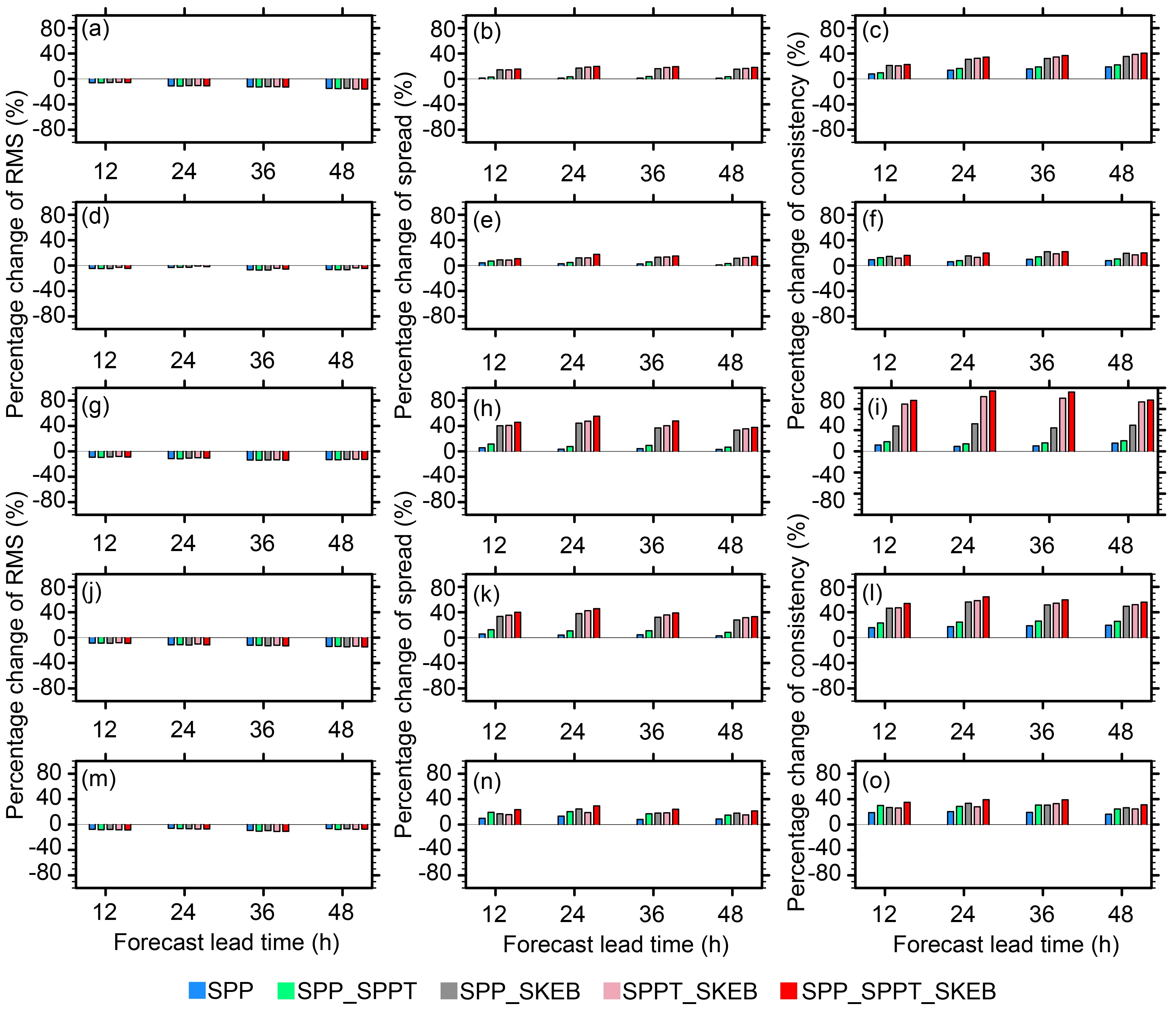 Figure7. Percentage change of (a, d, g, j, m) ensemble mean RMSE, (b, e, h, k, n) ensemble spread and (c, f, i, l,o) consistency of the five stochastic experiments relative to the CTL experiment for (a, b, c) 250-hPa zonal wind speed, (d, e, f) 500-hPa temperature, (g, h, i) 850-hPa zonal wind speed, (j, k, l) 10-m zonal wind speed, and (m, n, o) 2-m temperature, varying with forecast hour. The results are the monthly average for the 0000 UTC cycle during June 2015.
Figure 7 shows that all the stochastic experiments reduce the RMSE and improve the ensemble spread and consistency compared to the CTL experiment. The RMSE is reduced by 5%–15% for all stochastic experiments (Figs. 7a, d, g, j, m). Compared to the SPP and SPP_SPPT experiments, the experiments with SKEB dramatically increase the ensemble spread by 15%–57% and improve the consistency by 20%–100%, and the SPP_SPPT_SKEB experiment is characterized by the highest improvements for the ensemble spread and consistency, especially for the 250-hPa (Figs. 7a, b, c), 850-hPa (Figs. 7g, h, i) and 10-m (Figs. 7j, k, l) zonal wind speed. The improvement for temperature is comparatively small. For the 500-hPa temperature (Figs. 7d, e, f) and 2-m temperature (Figs. 7m, n, o), the five stochastic experiments show a slightly better spread and consistency than the CTL experiment, indicating a slight improvement for temperature (by about 2%–30%). For almost every variable and lead time, all the experiments are characterized by spread values well below their corresponding RMSE, except for 250-hPa wind speed (not shown here), indicating that almost all the experiments are underdispersive. This can be seen in the corresponding domain-averaged consistency (Fig. 7, right-hand panels), where the consistency value is < 1.0 for almost all experiments. The domain-averaged consistency of the 250-hPa (Fig. 7c) and 850-hPa (Fig. 7i) wind speed in the SPP_SPPT_SKEB scheme shows a dramatic improvement compared to the CTL experiment and the SPP experiment, while for the 500-hPa temperature (Fig. 7d) and 2-m temperature (Fig. 7o), the improvement is not so dramatic but only slight, which may due to the systematic bias for 500-hPa and 2-m temperature that can be seen in Figs. 9c and k.
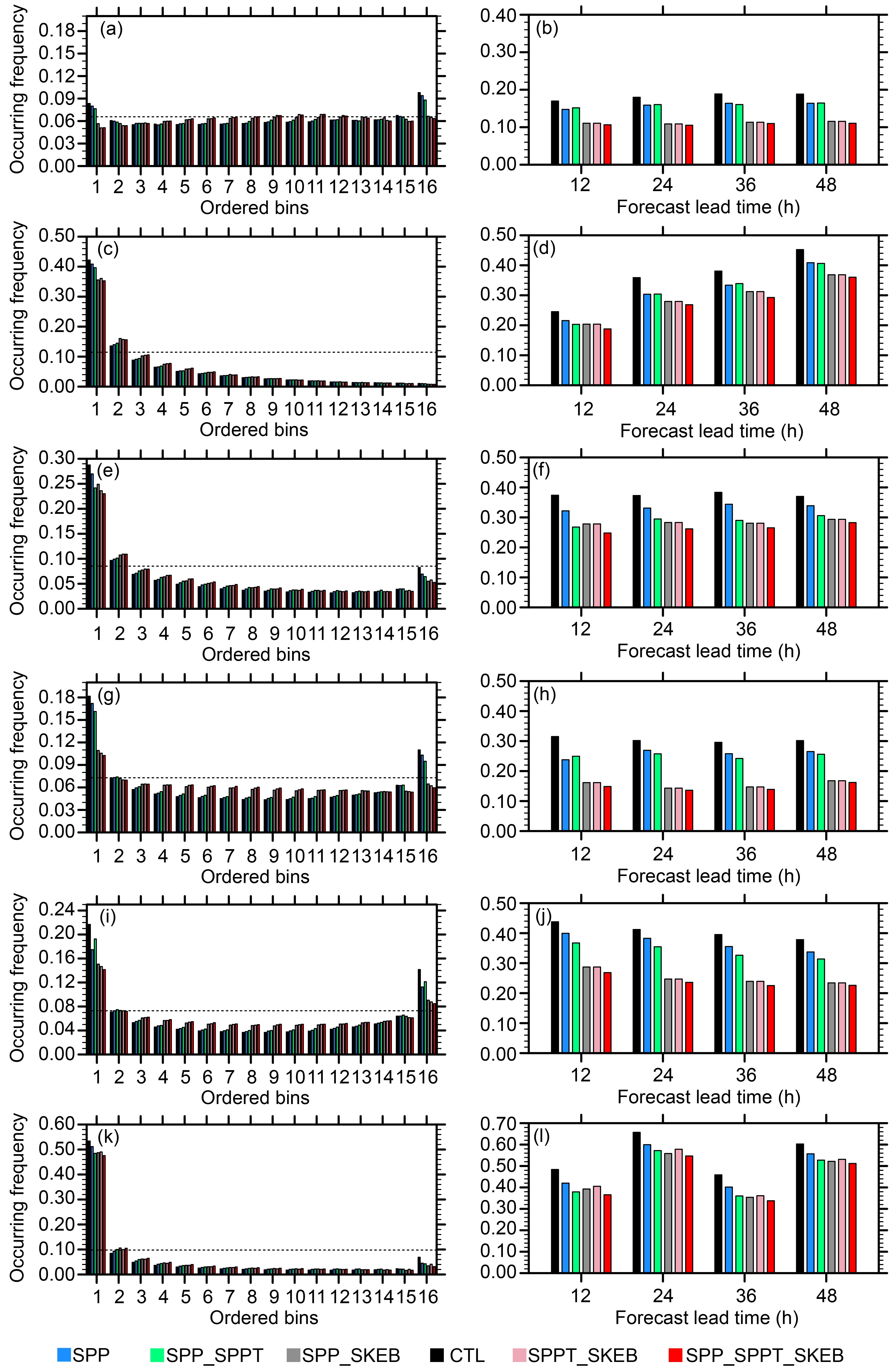 Figure9. Rank histograms and outlier scores at the 48-h forecast lead time for (a, b) 250-hPa zonal wind speed, (c, d) 500-hPa temperature, (e, f) 850-hPa temperature, (g, h) 850-hPa zonal wind speed, (i, j) 10-m zonal wind speed, and (k, l) 2-m temperature, varying with forecast hour. The results are the monthly average for the 0000 UTC cycle during June 2015.
These results show that both the spread and consistency are dramatically improved by the SPP_SPPT_SKEB scheme without increasing the forecast mean error. Therefore, the overall forecast skill is improved, resulting in a more reliable EPS. The improvement is more dramatic for the winds than the temperature, which may be due to the reason that the SKEB scheme, which only acts on the wind field and does not affect the temperature field, contributes most to the improvement in the spread of the wind speed. The improvement in spread and consistency between the CTL and the SPP_SPPT_SKEB experiments is statistically significant at the 99.99% level (t-test) for all verified variables, although the difference in the RMSE is not statistically significant.
The CRPS is also calculated to measure the absolute error between the forecast probability and the observations (Hersbach, 2000). Note that lower values of CRPS denote a better forecast skill. Figure 8 shows percentage improvements of CRPS of the five stochastic experiments relative to the CTL experiment. In comparison with the CTL experiment, all experiments reduced the CRPS by about 1%–6%, indicating an improvement of the probabilistic forecast skill. Furthermore, the SPP_SPPT_SKEB experiment is characterized by the largest improvements of CRPS (highest skill) compared with the other experiments for most of the variables and lead times, which implies a better performance. Note that the difference in CRPS between the CTL and SPP_SPPT_SKEB experiments is statistically significant at the 95% level (t-test) for the lead times for all verified variables.
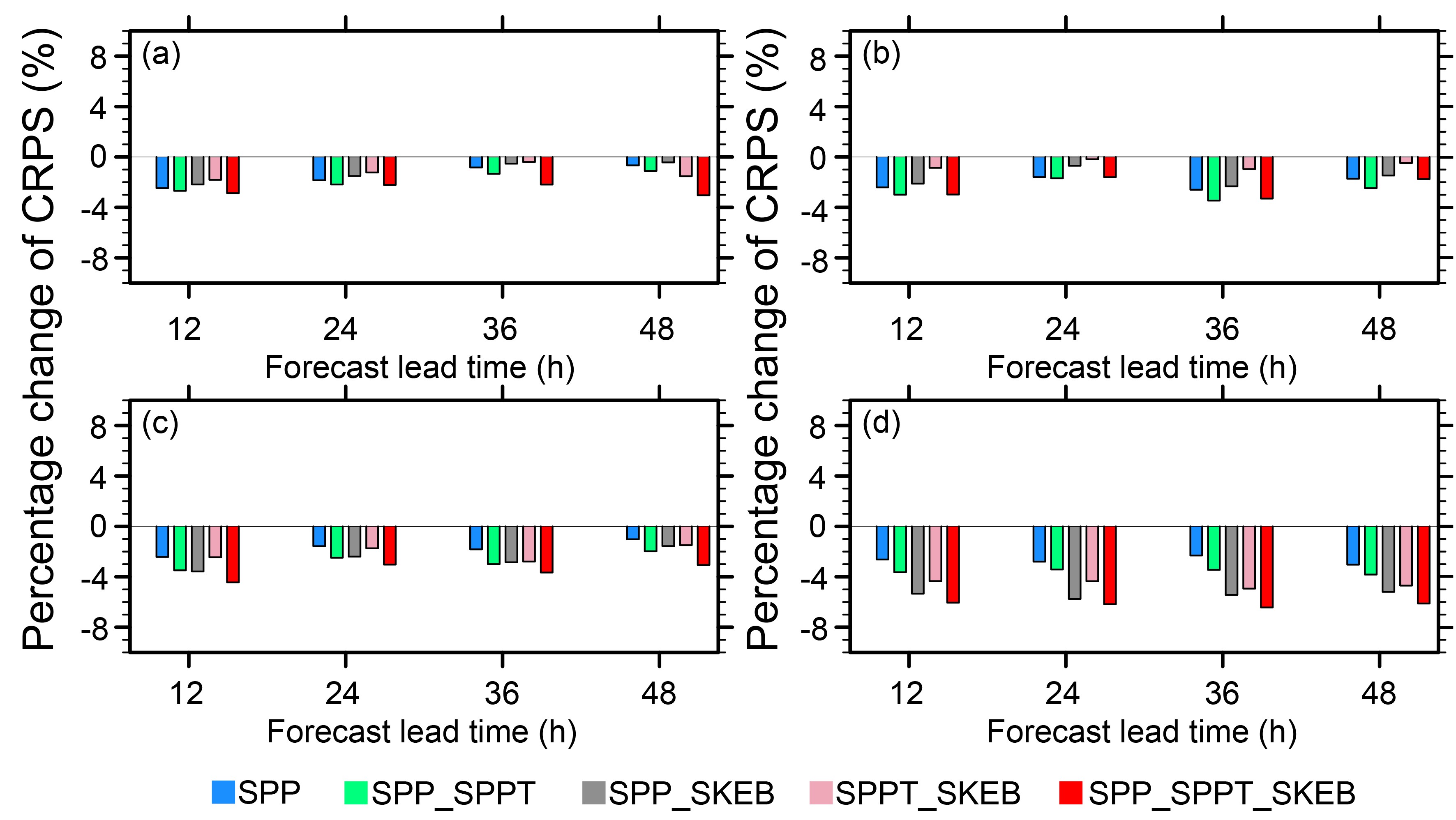 Figure8. Percentage change of CRPS of the five stochastic experiments relative to the CTL experiment for (a) 250-hPa zonal wind speed, (b) 500-hPa temperature, (c) 850-hPa zonal wind speed, and (d) 10-m zonal wind speed, varying with forecast hour. The results are the monthly average for the 0000 UTC cycle during June 2015.
The Talagrand distribution is also used to evaluate the ability to capture the observed data for an EPS by plotting the frequency of occurrence of observations in each bin (Talagrand et al., 1997; Hamill, 2001). A flat distribution is expected for an ideal EPS with n members (Wang et al., 2018). Figure 9 (left-hand panels) shows that the 250- (Fig. 9a) and 850-hPa (Fig. 9g) wind speeds are relatively flat, which implies that GRAPES-REPS can capture the observed data well. The SPP and SPP_SPPT experiments are underdispersive for 250-hPa wind speed (Fig. 9a), and the addition of SKEB flattens the rank histogram. The resulting rank histograms of the SPP_SPPT_SKEB, SPP_SKEB and SPPT_SKEB experiments are comparatively flat, indicating a better performance. However, there is a strong warm bias in the diagrams of the 500-hPa (Fig. 9c), 850-hPa (Fig. 9e) and 2-m temperatures (Fig. 9k), which is also reported in Wang et al. (2018). Figure 9 (right-hand panels) shows the outlier scores for the six experiments. The sum of the two end bins of the rank histograms (the outlier score) refers to the frequency at which the observations fall outside the ensemble envelope. Lower values indicate a more reliable distribution for an ensemble member. All the stochastic experiments are characterized by lower outlier scores than the CTL experiment for all thresholds and forecast lead times. The SPP_SKEB, SPPT_SKEB and SPP_SPPT_SKEB schemes are characterized by significantly lower outlier scores than the other three schemes for all variables, indicating a notable impact of SKEB on reducing the outlier score. The differences in the outlier scores between the CTL and the SPP_SPPT_SKEB experiments is statistically significant at the 99.9% level (t-test) for all lead times.
2
4.3. Analysis of the KE spectrum
Aiming to demonstrate the effect of introducing SPP, SPPT, and SKEB on the KE of each atmospheric wavelength, the KE spectrum, which can give the information about KE of each atmospheric wavelength, is analyzed. The KE spectrum is computed as a vertically integrated quantity over all model levels and then integrated across each wavelength, and for a unit mass of gas, the KE is given by:where the u and v represent the zonal and meridional wind speed, respectively and w represents the vertical speed. The KE is calculated for the ensemble mean, and the KE changes caused by introducing SPP, SPPT and SKEB are measured by the percentage changes of KE from experiment SPPT_SKEB to experiment SPP_SKEB_SPPT, and that from experiment SPP to experiment SPP_SPPT and SPP_SKEB, respectively.
As shown in Eq. (13), Eexp1 and Eexp0 correspond with the KE of experiment1 and experiment0, respectively. For comparison, the percentage change in Eexp1 to Eexp0 is defined as RAE. If RAE is positive, then the KE spectrum of experiment1 is larger than the KE spectrum of experiment0. If RAE is negative, then the opposite is true:
Figures 10a–c show the percentage change in the KE spectrum of SPP_SPPT_SKEB over SPPT_SKEB (Fig. 10a), SPP_SPPT over SPP (Fig. 10b), and SPP_SKEB over SPP (Fig. 10c) of the 500-hPa wind at a 48-h lead time. As shown in Fig. 10a, introducing SPP into the ensemble system results in a small change (less than ± 4%) of KE for all wavelengths, indicating that SPP does not lead to large changes in the evolution of the KE spectrum at any wavelength. For the percentage change in the KE spectrum of SPP_SPPT over SPP (Fig. 10b), it indicates that the introduction of SPPT results in a 5%–10% change in KE for wavelengths less than 1000 km, and causes smaller KE changes for larger wavelengths. Additionally, there is a notable KE change due to the introduction of the SKEB scheme, where the introduction of SKEB results in a 30%–80% change in KE for wavelengths less than 1000 km, and KE changes maximally up to 80% at a wavelength of approximately 200–400 km. This dramatic KE change caused by the SKEB scheme may have impacts on long-term model drift, which should be considered in future work. Additionally, it should be noted that the KE changes caused by the SKEB scheme are in line with the influencing mechanism of SKEB on KE, which injects KE into the model domain to counteract excessive energy dissipation coming from numerical diffusion and interpolation. In general, the introduction of SPP results in a relatively slight change of KE for all wavelengths compared to that of SPPT and SKEB, and the SKEB scheme exerts the most impact on the KE due to its nature. Note that the results of 250-hPa and 850-hPa winds are similar to those of the 500-hPa wind, and the results for lead times of 0, 12, 24, and 36 h are similar to those for the 48-h lead time, and thus they are not shown here.
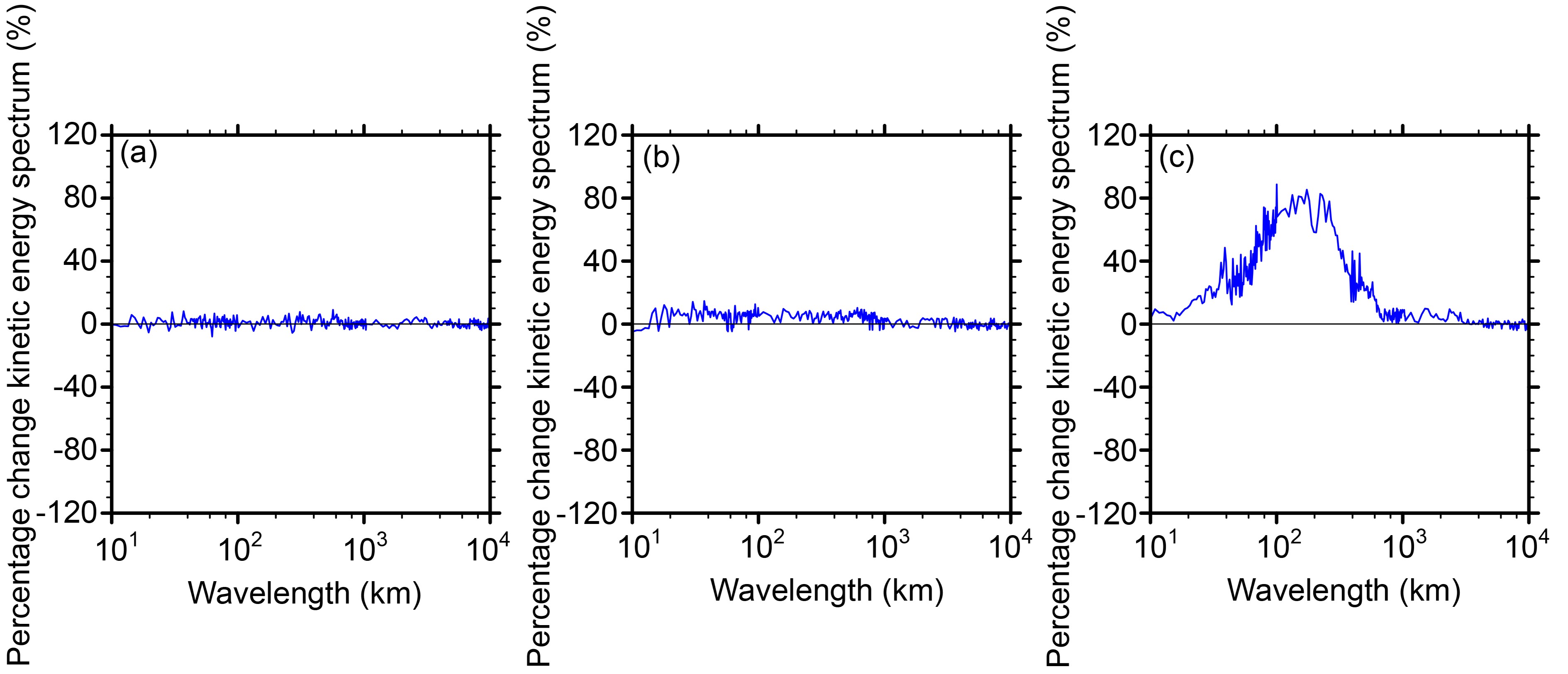 Figure10. Percentage change in the KE spectrum of (a) SPP_SPPT_SKEB over SPPT_SKEB, (b) SPP_SPPT over SPP, and (c) SPP_SKEB over SPP for the 500-hPa winds at a 48-h lead time. The results are the monthly mean for the 0000 UTC cycle during June 2015.
Figures 11a–c show the percentage change in the KE spectrum of SPP_SPPT_SKEB over SPPT_SKEB (Fig. 11a), SPP_SPPT over SPP (Fig. 11b), and SPP_SKEB over SPP (Fig. 11c) of five typical wavelengths characterized by representative synoptic meanings: 20 km (meso-


 Figure11. Percentage change in the KE spectrum of (a) SPP_SPPT_SKEB over SPPT_SKEB, (b) SPP_SPPT over SPP, and (c) SPP_SKEB over SPP for five typical and representative wavelengths varying with forecast hour. The results are the monthly mean for the 0000 UTC cycle during June 2015.
2
4.4. Added value of the SPP scheme
The verification results shown above indicate that the best results are achieved when combining all three stochastic schemes (SPP, SPPT and SKEB), and many previous studies have proven the beneficial impacts of SPPT and SKEB (e.g., Berner et al., 2009, Palmer et al., 2009). But how does SPP perform in the combined scheme? To investigate the added value of the SPP scheme to combinations with the SPPT and SKEB schemes, the verification scores of SPP_SPPT_SKEB were compared with that of the SPPT_SKEB scheme. Figure 12 shows the percentage change in SPP_SPPT_SKEB over SPPT_SKEB for different verification metrics.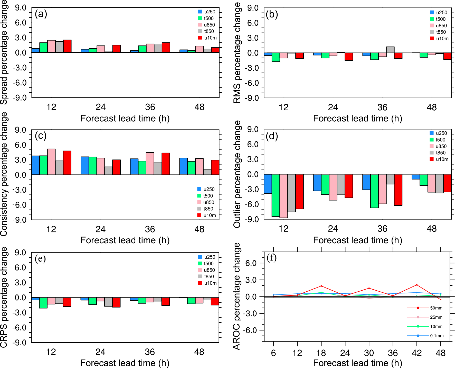 Figure12. Percentage change of the SPP_SPPT_SKEB scheme over the SPPT_SKEB scheme in (a) spread, (b) RMSE, (c) consistency, (d) outliers, and (e) CRPS, for 250-hPa zonal wind speed (blue), 500-hPa temperature (green), 850-hPa temperature (gray), 850-hPa zonal wind speed (pink), and 10-m zonal wind speed (red), as well as (f) AROC scores for precipitation verification, varying with forecast hour.
For almost every variable and forecast lead time, the introduction of SPP results in a positive improvement in spread (Fig. 12a) and consistency (Fig. 12c) and a reduction in the RMSE (Fig. 12b). The CRPS (Fig. 12d) and outlier score (Fig. 12e) also decrease. The AROC (Fig. 12g) is improved, indicating a positive added value in precipitation forecasts. This analysis shows that introducing SPP is generally beneficial in improving the overall performance of these experiments.
(1) All stochastic experiments outperform the CTL experiment, and all combinations of stochastic parameterization schemes perform better than the single scheme SPP, indicating that stochastic methods can effectively improve the forecast skill, and combinations of stochastic parameterization schemes can better represent the model uncertainties.
(2) The combination of all three stochastic physics schemes (SPP, SPPT, and SKEB) outperforms any other combination of two schemes in precipitation forecasting and surface and upper-air verification, indicating that the model uncertainties can be better represented by a combination of SPP, SPPT, and SKEB.
(3) Combining SKEB with SPP and/or SPPT results in a notable increase in spread and reduction in outliers for the upper-air wind speed. SKEB directly perturbs the wind field and therefore its addition will greatly impact the upper-air wind-speed fields, and it contributes most to the improvement in spread and outliers for wind.
(4) Analysis of the added value of SPP showed that combining SPP with SPPT and SKEB generally generates a positive improvement in the ensemble spread, RMSE, consistency, CRPS, and the outlier and AROC scores for precipitation verification over the SPPT_SKEB scheme, indicating that introducing SPP contributes to the overall performance. This may be explained by the perturbation of various uncertain parameters affecting critical processes, such as: the turbulent mixing of moisture, momentum and heat in the boundary layer; the entrainment and downdraft at the top of the boundary layer; the vertical diffusion above the boundary layer; deep, mid-level and shallow convection; cloud formation; cloud-top diffusion; and the auto-conversion of cloud water to rain. More uncertainties can therefore be represented and a greater number of parameter values explored during the forecast, thereby improving the forecast skill and reducing the forecast error.
(5) Introducing SPP does not lead to large changes in the evolution of the KE spectrum at any wavelength (the percentage change in the KE spectrum is less than ± 4% for all wavelengths), and the introduction of SPPT and SKEB would cause a 5%–10% and 30%–80% change in the KE of mesoscale systems, respectively. Note that there is a notable KE change (may up to 80%) due to the introduction of the SKEB scheme, and this dramatic KE change may have impacts on long-term model drift, which should be considered in future work.
(6) In general, all three stochastic schemes (SPP, SPPT, and SKEB) mainly exert an influence on the KE of mesoscale systems.
This study suggests that combinations of multiple stochastic physics schemes deal better with model uncertainties and confirm the findings of previous studies (Berner et al., 2011, 2015; Hacker et al., 2011a, b; Jankov et al., 2017) in that model error can be better represented by a combination of model-error schemes than a single scheme alone. In addition, this study highlights the positive potential of SPP to be developed further in the future—the introduction of SPP is generally beneficial in improving the overall performance. Our ?nding lays a foundation for the development and design of next-generation regional and global ensembles, and future work is progressing in the investigation of whether a single-physics suite combined with multiple stochastic perturbations (SPP, SPPT, and SKEB) can outperform and be used as an alternative to operational multiphysics schemes.
Acknowledgements. We are grateful to four anonymous reviewers for their positive and constructive suggestions and comments. This work was sponsored by National?Key?Research?and?Development?(R?&?D)?Program?of?China,?(Grant?No.?2018YFC1507405)?.
