HTML
--> --> -->Global highlands have great influence on global monsoons. Previous studies suggest that highlands, especially the Tibetan–Iranian Plateau (TIP) highlands over the Asian continent, could exert both mechanical and thermal forcings on the surrounding atmosphere and lead to changes in the global monsoon system and hydrological cycle (Queney, 1948; Hahn and Manabe, 1975; Kitoh, 1997; Abe et al., 2003; Liu et al., 2007; Okajima and Xie, 2007; Wu et al., 2007; Zhou et al., 2009c). However, debate still exists on how the TIP modulates the Asian monsoon system (Boos and Kuang, 2010, 2013; Wu et al., 2012; He et al., 2015; Wu et al., 2015). The different understandings of the effect of the TIP climate originate from both the lack of observation datasets and limitations to the simulation ability of climate models.
The Global Monsoons Model Intercomparison Project (GMMIP) is one of the endorsed MIPs in the sixth phase of the Coupled Model Intercomparison Project (CMIP6). It designed a series of extended Tier-1 Atmospheric Model Intercomparison Project (AMIP) experiments to understand the behavior of monsoon circulations and associated precipitation over the late 19th through the early 21st centuries. It also designed Tier-3 orographic perturbation experiments to quantitatively understand the regional response to orographic perturbation from both thermal and dynamic aspects (Zhou et al., 2016). In addition to the TIP orography, the Tier-3 experiments also included orographic perturbation experiments, including experiments over the East African highlands, North American highlands, and South American highlands.
The Chinese Academy of Sciences (CAS) Flexible Global Ocean–Atmosphere–Land System (FGOALS-f3-L) climate system model, which was developed at the Institute of Atmospheric Physics (IAP)/State Key Laboratory of Numerical Modeling for Atmospheric Sciences and Geophysical Fluid Dynamics (LASG) (Zhou et al., 2012, 2015; Bao et al., 2019), recently finished GMMIP Tier-1 and Tier-3 simulations. To provide an essential model configuration and experimental method for a variety of users, we provide detailed descriptions of the model design and data outputs of the GMMIP Tier-1 and Tier-3 experiments by the CAS FGOALS-f3-L model in this study. Section 2 presents the model description and experimental design. Section 3 shows the technical validation of the FGOALS-f3-L experiments. Section 4 provides usage notes.
2.1. Model introduction
The configuration of the CMIP6 version of the CAS FGOALS-f3-L model is introduced in the description paper of the AMIP datasets (He et al., 2019). For convenience for those using only the GMMIP datasets, we briefly reintroduce the model here. The CAS FGOALS-f3-L model is structured with five components: version 2.2 of the Finite-volume Atmospheric model (FAMIL) (Zhou et al., 2015; Bao et al., 2019; Li et al., 2019), which is the next generation atmospheric general circulation model (AGCM) Spectral Atmospheric Model (SAMIL) (Wu et al., 1996; Bao et al., 2010, 2013); version 3 of the LASG/IAP Climate system Ocean Model (LICOM3) (Liu et al., 2012); version 4.0 of the Community Land Model (CLM4) (Oleson et al., 2010); and version 4 of the Los Alamos sea ice model (CICE4) (Hunke et al., 2010). The fluxes are exchanged between these components using version 7 of the coupler module from the National Center for Atmospheric Research (NCAR) (The atmospheric component of FAMIL adopts a three-dimensional finite-volume dynamical core (Lin, 2004) over cubed-sphere grids (Putman and Lin, 2007) with six tiles over the globe. In the CAS FGOALS-f3-L model, each tile contains 96 grids (C96). For the globe, the longitudinal extent is divided into 384 grids, and the latitudinal area is divided into 192 grids, which results in an approximate 1° horizontal resolution. In the vertical direction, the model adopts hybrid coordinates with 32 layers, where the model top is 2.16 hPa. The main physical packages include a new moisture turbulence parameterization scheme for the boundary layer (Bretherton and Park, 2009), with shallow convection updated (Wang and Zhang, 2014). The GFDL (Geophysical Fluid Dynamics Laboratory) version of the single-moment six-category cloud microphysics scheme (Lin et al., 1983, Harris and Lin, 2014) is adopted to predict the bulk contents of water vapor, cloud water, cloud ice, rain, snow and graupel. For the cloud fraction diagnosis, the Xu and Randall (1996) scheme is used, which considers not only relative humidity but also the cloud mixing ratio, thus providing a more precise cloud fraction. A resolved convective precipitation parameterization (?2017 FAMIL Development Team) is used where, in contrast to conventional convective parameterization, convective and stratiform precipitation are calculated explicitly. In addition, a gravity wave drag scheme is also considered (Palmer et al., 1986).
2
2.2. Experiments
For the GMMIP Tier-1 experiments, three AMIP-type experiments are conducted, as summarized in Table 1. In these experiments, external forcings are prescribed as their monthly mean observation values, as recommended by previous CMIP6 projects: historical greenhouse gas concentrations from Meinshausen et al. (2017); solar forcing from Matthes et al. (2017); historical ozone concentrations from| Experiment_id | Variant_label | Integration time | Experimental design | |
| Tier-1 | amip-hist | r1i1p1f1 | 1861–2014 | The model integration starts from 1 January 1861 with the external forcings, including greenhouse gases, solar irradiance, ozone, aerosols, SSTs and sea ice, as defined by the observed values. The first nine integration years are recognized as the spin-up time, and the outputs from 1870 to 2014 are provided for analysis. |
| amip-hist | r2i1p1f1 | 1862–2014 | Same as r1i1p1f1, but the first eight integration years are recognized as the spin-up time, and the outputs from 1870 to 2014 are provided for analysis. | |
| amip-hist | r3i1p1f1 | 1863–2014 | Same as r1i1p1f1, but the first seven integration years are recognized as the spin-up time, and the outputs from 1870 to 2014 are provided for analysis. | |
| Tier-3 | amip-TIP | r1i1p1f1 | 1970–2014 | The topography above 500 m is set to 500 m in a polygon region. The coordinates of the polygon corners are as follows: longitude coordinates (from west to east) are 25°E, 40°E, 50°E, 70°E, 90°E and 180°E; latitude coordinates (from south to north) are 5°N, 15°N, 20°N, 25°N, 35°N, 45°N and 75°N. The model integration starts on 1 January 1970, which is the same as that in the amip r1i1p1f1 experiment. The outputs from 1979 to 2014 are provided for analysis. |
| amip-TIP-nosh | r1i1p1f1 | 1970–2014 | Sensible heating is removed from topographies above 500 m, as in the same polygon region in amip-TIP. One practical method is to set the vertical temperature diffusion term to zero in the atmospheric thermodynamic equation at the bottom boundary layer. The model integration is the same as above. | |
| amip-hld | r1i1p1f1 | 1970–2014 | Topographies of the East African Highlands in Africa and the Arabian Peninsula are modified by setting surface elevations to a certain height (500 m) in separate experiments. The East African highlands are in a polygon region. The coordinates of the polygon are as follows: longitude coordinates (from west to east) are 27°E and 52°E; latitude coordinates (from south to north) are 17°S, 20°N and 25°N, 35°N. The model integration is the same as above. | |
| amip-hld | r1i1p1f2 | 1970–2014 | The topography of the Sierra Madre in North America is modified by setting surface elevations to a certain height (500 m) in separate experiments. The Sierra Madre domain is (15°–30°N, 120°–90°W). The model integration is the same as above. | |
| amip-hld | r1i1p1f3 | 1970–2014 | The topography of the Andes in South America is modified by setting surface elevations to a certain height (500 m) in separate experiments. The Andes domain is (40°S–10°N, 90°–60°W). The model integration is the same as above. |
Table1. Experimental design.
In the first “amip-hist” experiment, “r1i1p1f1”, model integration starts from 1 January 1861 with the defined observations. The first nine integration years are recognized as the spin-up time, and the outputs from 1870 to 2014 are provided for analysis. The next two simulations, “r2i1p1f1” and “r3i1p1f1”, are the same as “r1i1p1f1” but with different initial times.
Following the design of the GMMIP Tier-3 experiments (Zhou et al., 2016), five AMIP-type experiments are conducted, as summarized in Table 1. All experiments are integrated from 1970 to 2014, where the first nine years are considered as the spin-up time, and the results from 1979 to 2014 are provided for analysis. These experimental settings are the same as those for the AMIP r1i1p1f1 experiment in DECK (the Diagnostic, Evaluation and Characterization of Klima), as documented in He et al. (2019).
The specific differences among the Tier-3 experiments are summarized as follows: In the first experiment (amip-TIP), the topography above 500 m is set to 500 m in the TIP region during integration. The specific coordinates of the polygon corners are also shown in Table 1. Moreover, the land use and other land surface properties remain unchanged in the land model. In the second experiment (amip-TIP-nosh), the model topography is defined by the original values, but the TIP surface is not allowed to heat the atmosphere. That is, in the boundary layer scheme, the vertical diffusion heating term is set to zero within the same polygon region where the topography is above 500 m, as it is in amip-TIP. In the third experiment (amip-hld r1i1p1f1), the topographies of the East African Highlands in Africa and the Arabian Peninsula, Sierra Madre in North America, and Andes in South America are modified by setting the surface elevations to a certain height (500 m). The coordinates of the polygon region are shown in Table 1. In the fourth (r1i1p1f2) and fifth (r1i1p1f3) experiments, the topography of the Sierra Madres in North America and the Andes in South America is modified by setting the surface elevation to a certain height (500 m), respectively.
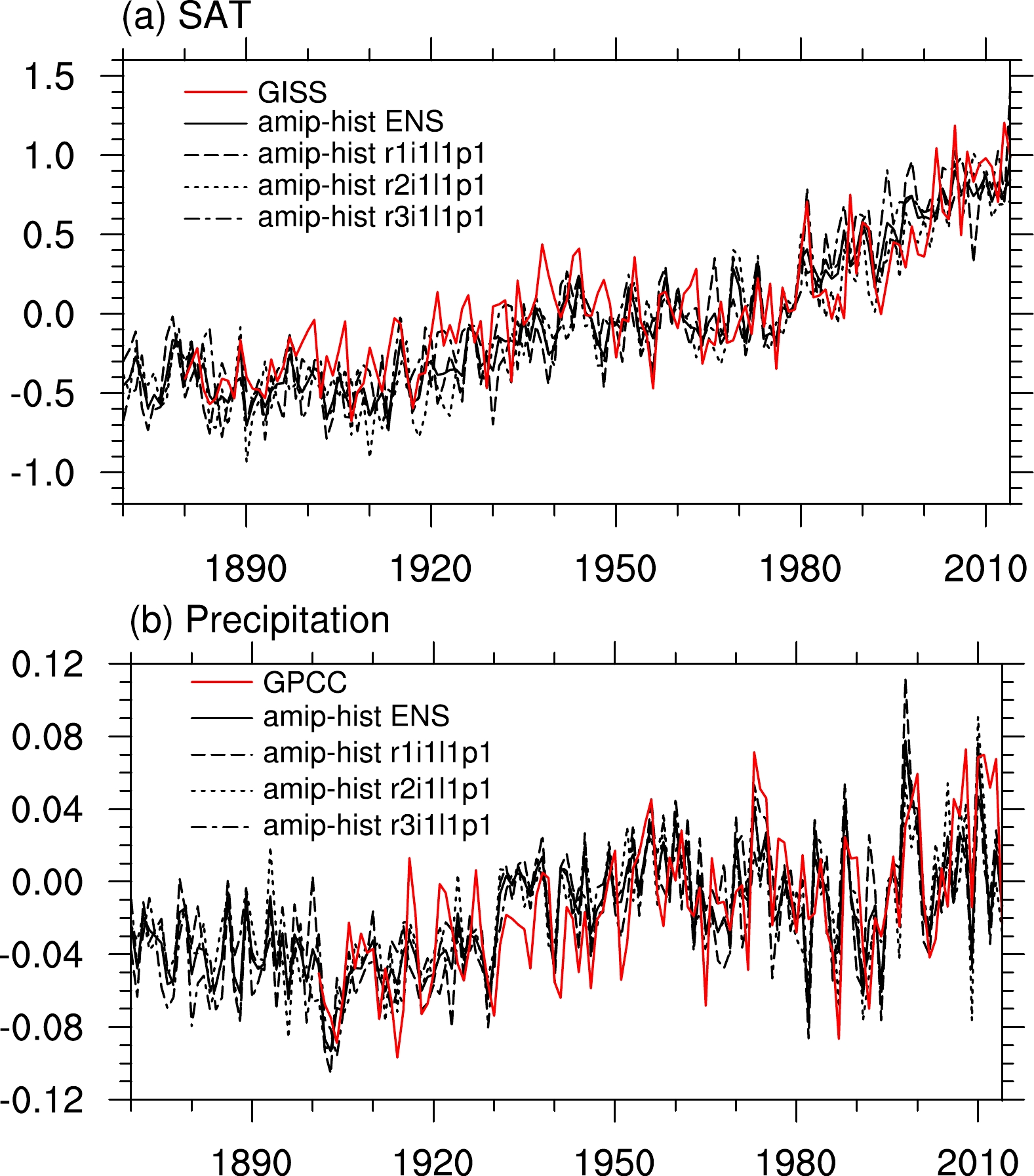 Figure1. (a) Time series of the global mean land SAT anomalies (units: K; relative to the mean values over 1951–1980). The red line denotes GISS datasets. The thick black line denotes the ensemble mean of the three amip-hist simulations, and the three kinds of dashed lines represent the three ensemble members: r1i1p1f1, r2i1p1f1, and r3i1p1f1. (b) As in (a) but for precipitation (units: mm d?1). The red line denotes the GPCC datasets.
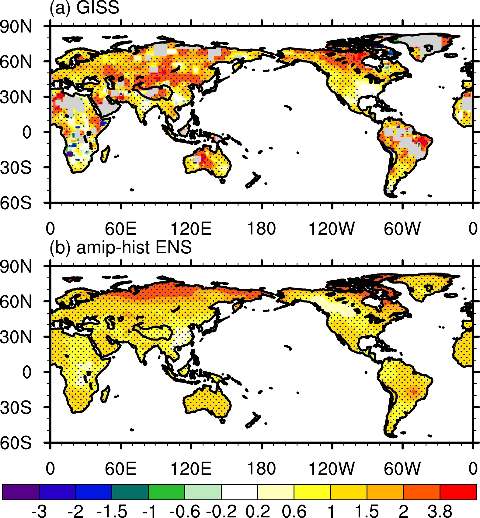 Figure2. Linear trends (1901–2014) of the global mean land SAT anomalies [units: K (115 yr)?1]: (a) GISS datasets; (b) ensemble mean of the three amip-hist simulations. The blue dots denote the values that have passed the 95% significance t-test. The black contour denotes the 3000-m topographic height.
 Figure3. Linear trends (1901–2014) of the global mean land precipitation anomalies [units: mm d?1 (115 yr)?1]: (a) GPCC datasets; (b) ensemble mean of the three amip-hist simulations. The red dots denote the values that have passed the 95% significance t-test. The black contour denotes the 3000-m topographic height.
Validation of the orographic perturbation experiments is also justified in this section. To check whether we have correctly carried out the sensitivity experiments, we show all five orographic forcings from the model outputs in Fig. 4. In the thermal perturbation experiment (amip-TIP-nosh), the topography in the model is unchanged; therefore, the topography height is realistic (Fig. 4b) and similar to that in Fig. 5 in Zhou et al. (2016), which was produced by HadGEM3 (the Met Office Hadley Centre Global Environmental Model, version 3). In the amip-TIP run (Fig. 4a), the TIP region, where the topography height is above 500 m, is correctly set to 500 m following the experimental design in Table. 1. Similarly, in amip-hld r1i1p1f1 (Fig. 4c), the polygon region in East Africa and the Arabian Peninsula is set to 500 m; in amip-hld r1i1p1f2 (Fig. 4d), the Sierra Madre is set to 500 m; in amip-hld r1i1p1f3 (Fig. 4d), the Andes is set to 500 m. These orographic perturbations exactly follow the GMMIP Tier-3 design [Fig. 5 in Zhou et al. (2016)]. In the thermal perturbation experiment (amip-TIP-nosh), the vertical diffusion heating is set to zero throughout the integration above 500 m. We show the climatological mean (1979–2014) vertical diffusion heating of amip-TIP-nosh in Fig. 5. It is clear that in the TIP region, which is contoured by the thick black line (500 m in Fig. 5), the vertical diffusion heating is zero, which suggests that our sensitivity experiments have been carried out correctly.
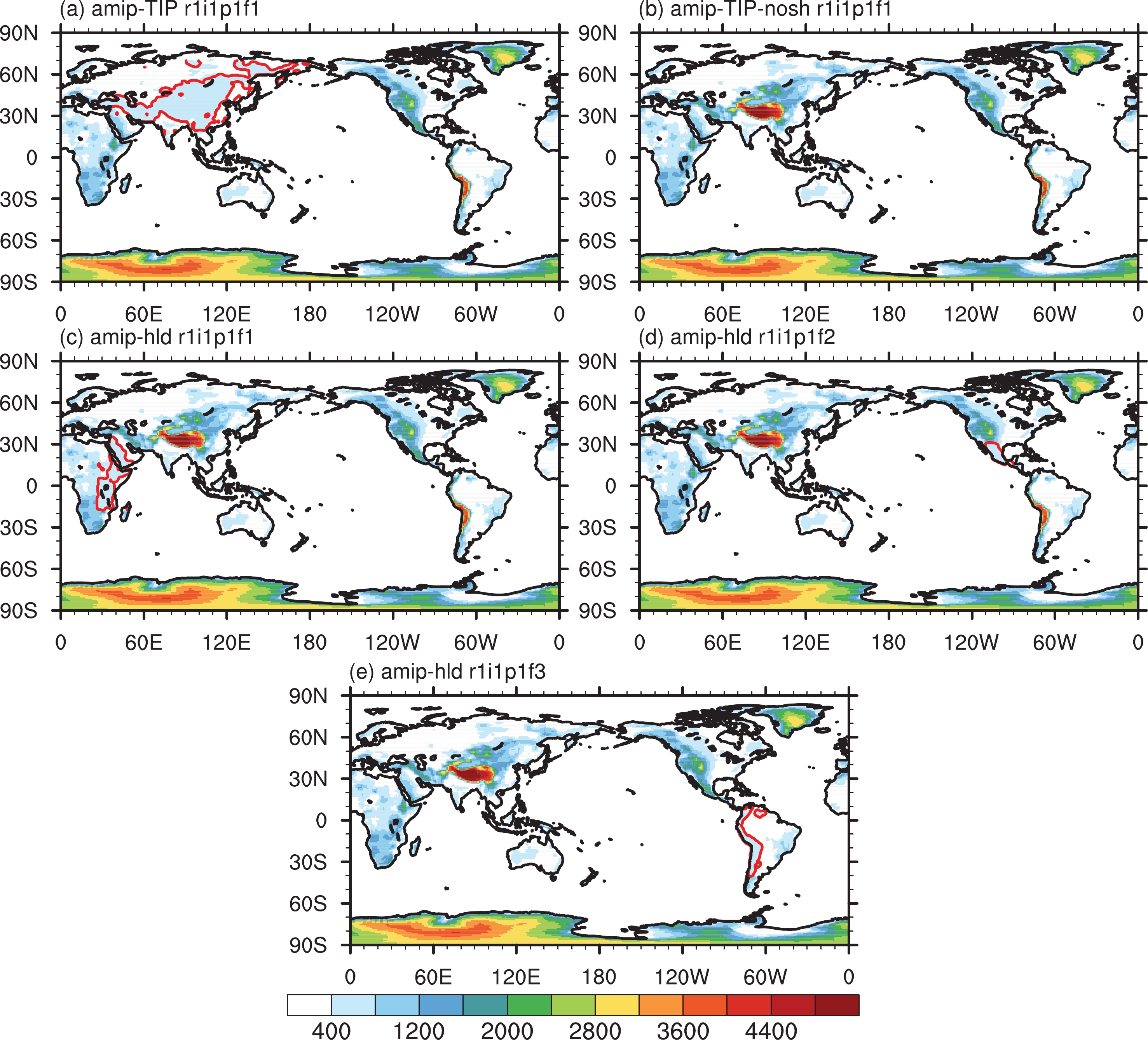 Figure4. Topography heights (shaded; units: m) in the experiments of (a) no TIP topography experiment amip-TIP, (b) no TIP sensible heating experiment amip-TIP-nosh, (c) no East African Highlands in Africa and the Arabian Peninsula experiment amip-hld r1i1p1f1, (d) no Sierra Madre experiment amip-hld r1i1p1f2, and (e) no Andes experiment amip-hld r1i1p1f3. The red contours denotes the modified topography.
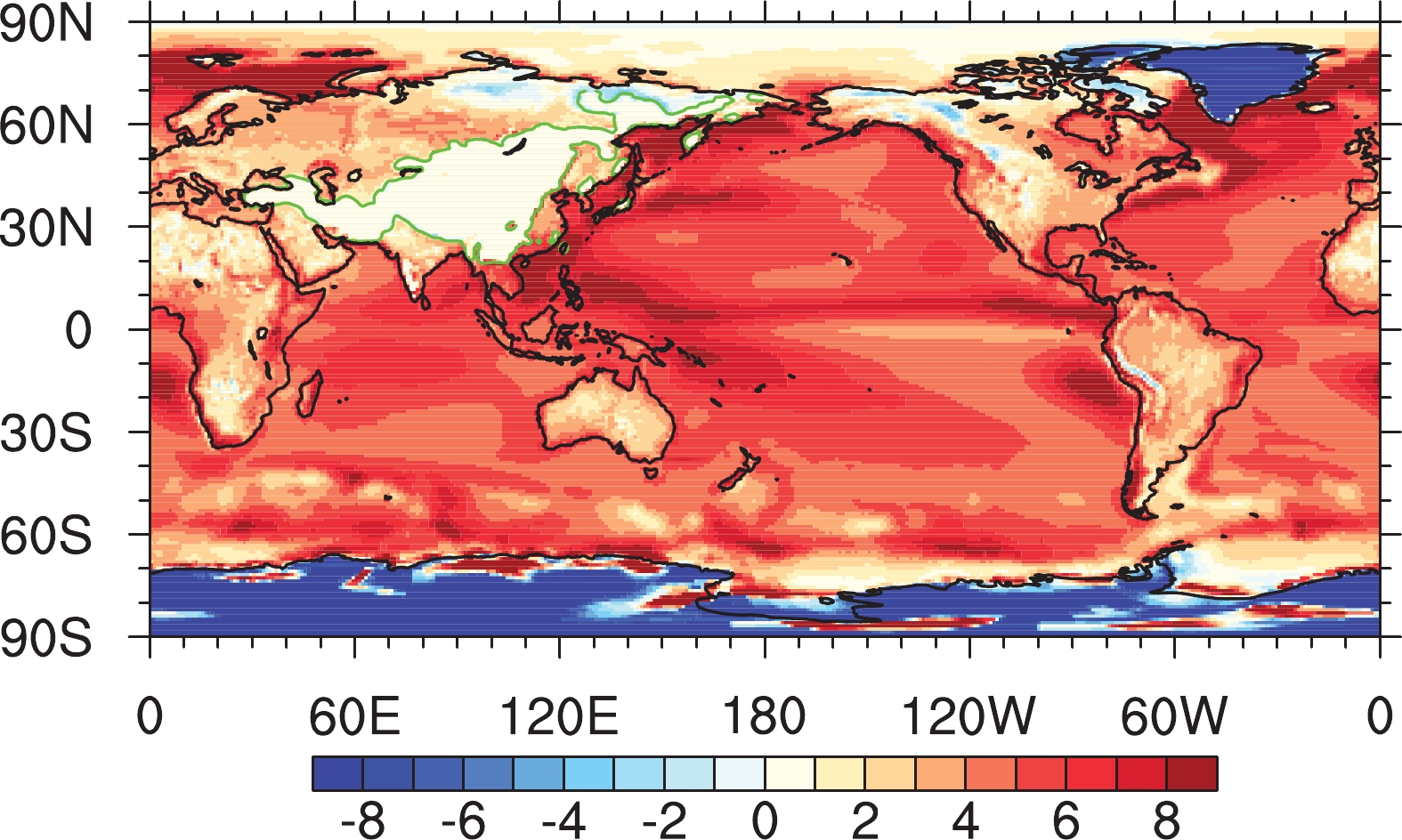 Figure5. Climatological mean (1979–2014) of vertical diffusion heating (shaded; units: K d–1) at the surface in amip-TIP-nosh. The thick black contour denotes the 500-m topographic height. The green contour denotes the region where the vertical diffusion heating is modified.
To understand the possible influence of TIP thermal and mechanical forcings on extreme events and its use in downscaling studies, potential uses may need to compare these experiments to the reference run. We recommend the CMIP6 DECK AMIP r1i1p1f1 experiment by using the CAS FGOALS-f3-L model as the reference run since these experiments share the same model and have a consistent integration method and initial state (He et al., 2019). Here, we show the climate mean responses of the TIP thermal and dynamical effect on the Asian summer monsoon in Fig. 6. The difference of the June–July–August (JJA) precipitation and 850-hPa wind between amip r1i1p1f1 and amip-TIP-nosh r1i1p1f1 (Fig. 6a) shows a similar large-scale pattern as in previous studies (Fig. 3c in Wu et al., 2012), with positive precipitation anomalies over South Asia and the North Indian Ocean and negative precipitation anomalies over the tropical Indian Ocean accompanied by cyclonic circulation around the TP. The difference between amip r1i1p1f1 and amip-TIP r1i1p1f1 (Fig. 6b) also shows similar patterns as in Fig. 2a of Wu et al. (2012), which indicates that the previous conclusions that TP heating could induce a low-level cyclonic circulation anomaly are robust to a different climate model. In addition, there also exist regional differences between the current model results (Fig. 6) and previous model results (Wu et al., 2012). For example, the positive precipitation anomalies over the western Pacific extend to the middle Pacific in the current model (Fig. 6a) but are limited to over the western North Pacific in the previous model [Fig. 3c in Wu et al. (2012)]. The reduction of this type of uncertainty requires multimodel results from GMMIP Tier-3 experiments.
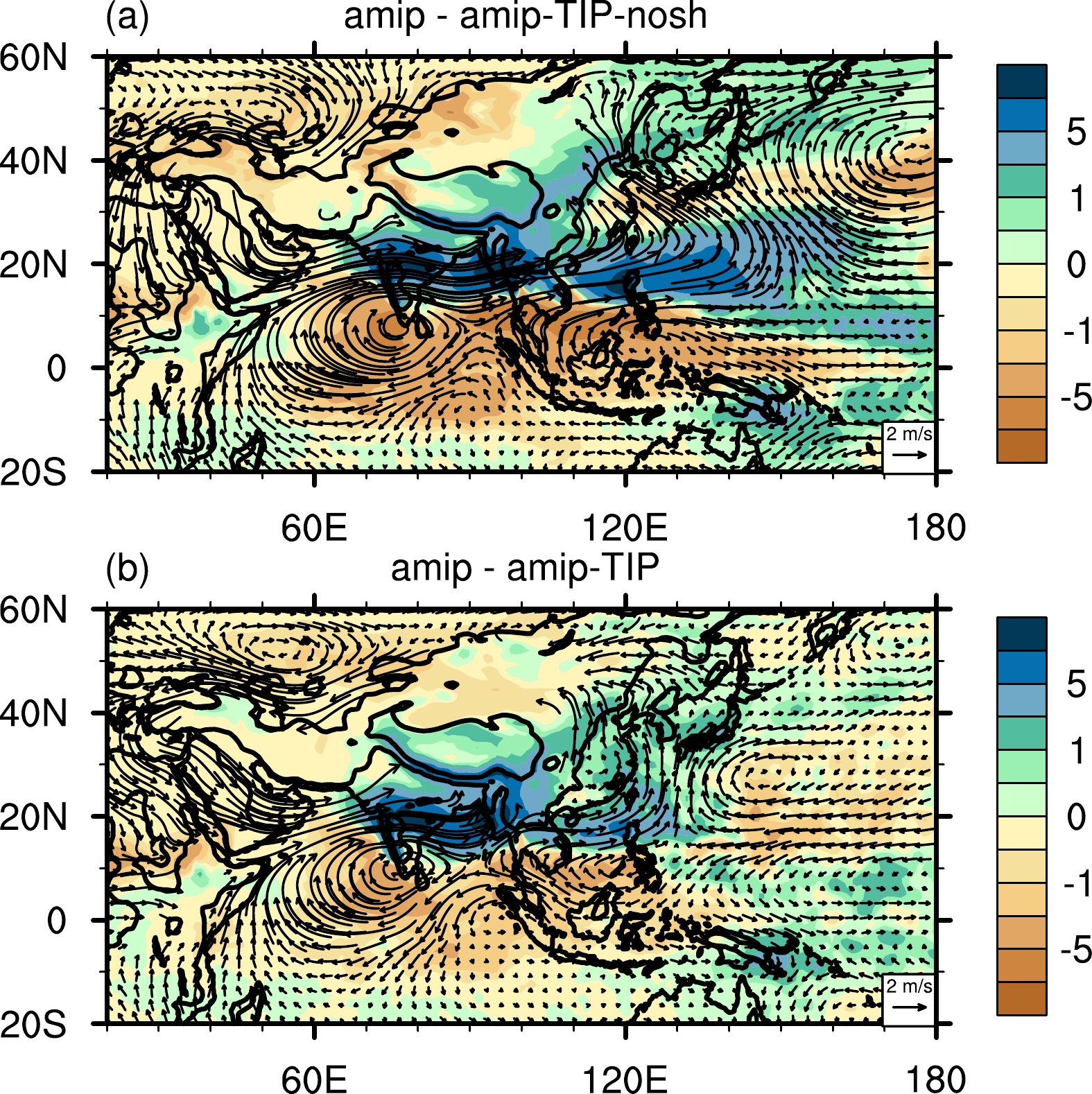 Figure6. Climatological (1979–2014) JJA mean precipitation (shaded; units: mm d–1) and 850-hPa wind (vectors; units: m s?1) differences between (a) amip r1i1p1f1 and amip-TIP-nosh r1i1p1f1, and (b) amip r1i1p1f1 and amip-TIP r1i1p1f1. The thick black contour denotes the 500- and 3000-m topographic heights, respectively.
The weather and climate change of the West Indian Ocean is important for countries in South Asia and East Africa (Goddard and Graham, 1999; Black et al., 2003), while the East African highlands are one of the topographies forcing climate change over the West Indian Ocean (Slingo et al., 2005). Here, we show the influences of the East African highlands by comparing experiments between amip r1i1p1f1 and amip-hld r1i1p1f1 in Fig. 7. Figure 7a shows the JJA differences of the precipitation and 850-hPa winds. A strong anticyclonic anomaly appears over the North Arabian Sea, leading to a strong easterly along the East coast of the tropical African continent. The precipitation anomaly shows a dipole pattern over the West Indian Ocean with decreases in the Arabian Sea and Bay of Bengal but an increase in the tropical central Indian Ocean. The precipitation over central Africa is also increased. The spatial patterns of precipitation and winds are similar to those in Fig. 7f and Fig. 8f of Slingo et al. (2005), who studied the influence of the East African Highlands by the Hadley Centre’s climate model (HadAM3). For December–January–February (DJF) (Fig. 7b), the East African Highlands induce cyclonic circulation over Northeast Africa and the Arabian Peninsula, accompanied by increased precipitation on the east of the cyclonic anomaly. In the Southern Hemisphere, the topographic forcing induces a northerly wind along the east coast of Africa, increased precipitation over the West Indian Ocean, and decreased precipitation over the East Indian Ocean, which are roughly similar to Figs. 7c and 8c in Slingo et al. (2005).
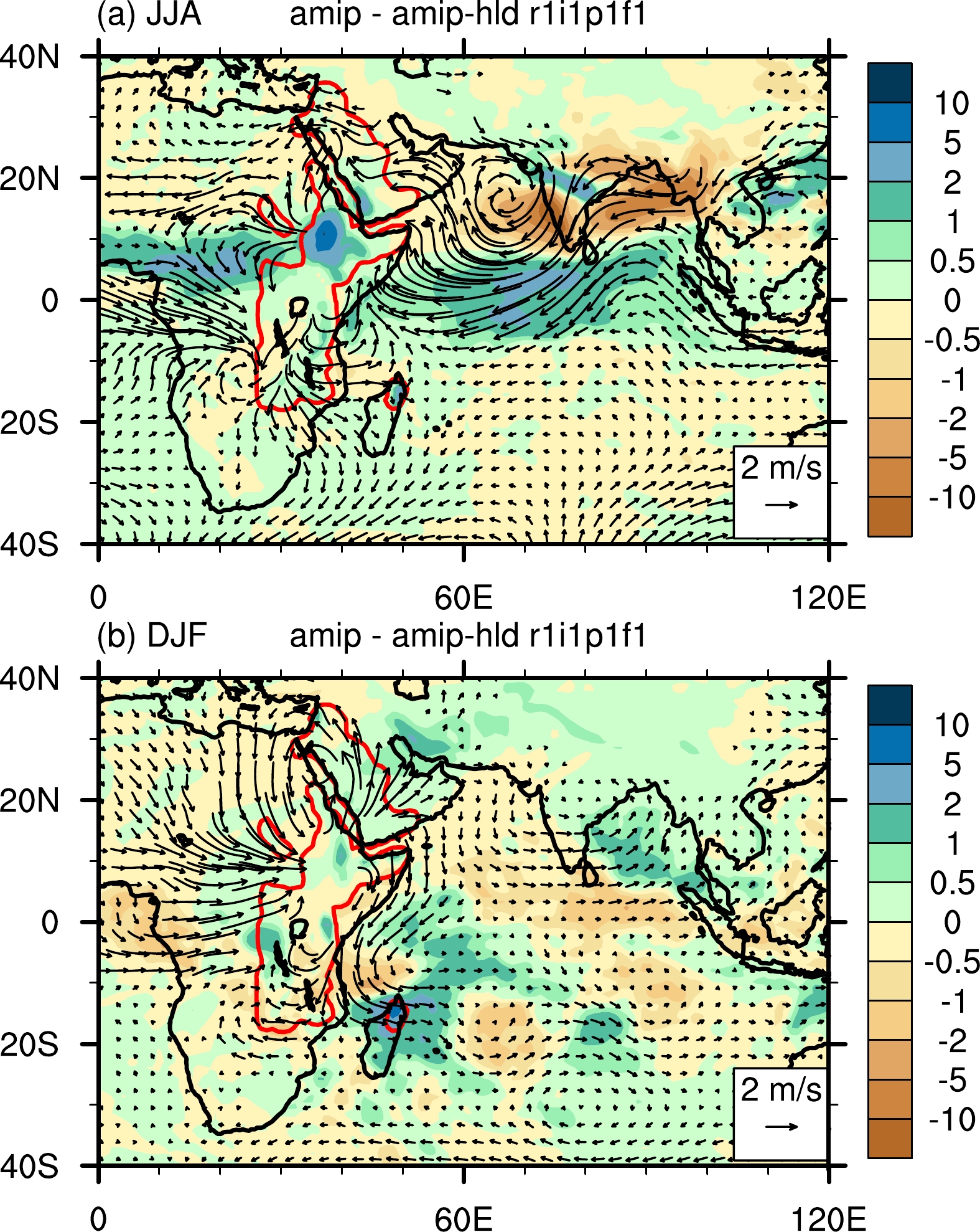 Figure7. (a) Climatological (1979–2014) JJA mean precipitation (shaded; units: mm d–1) and 850-hPa wind (vectors; units: m s?1) differences between amip r1i1p1f1 and amip-hld r1i1p1f1. (b) As in (a) but for the DJF mean. The red contour denotes the topography modified in amip-hld r1i1p1f1.
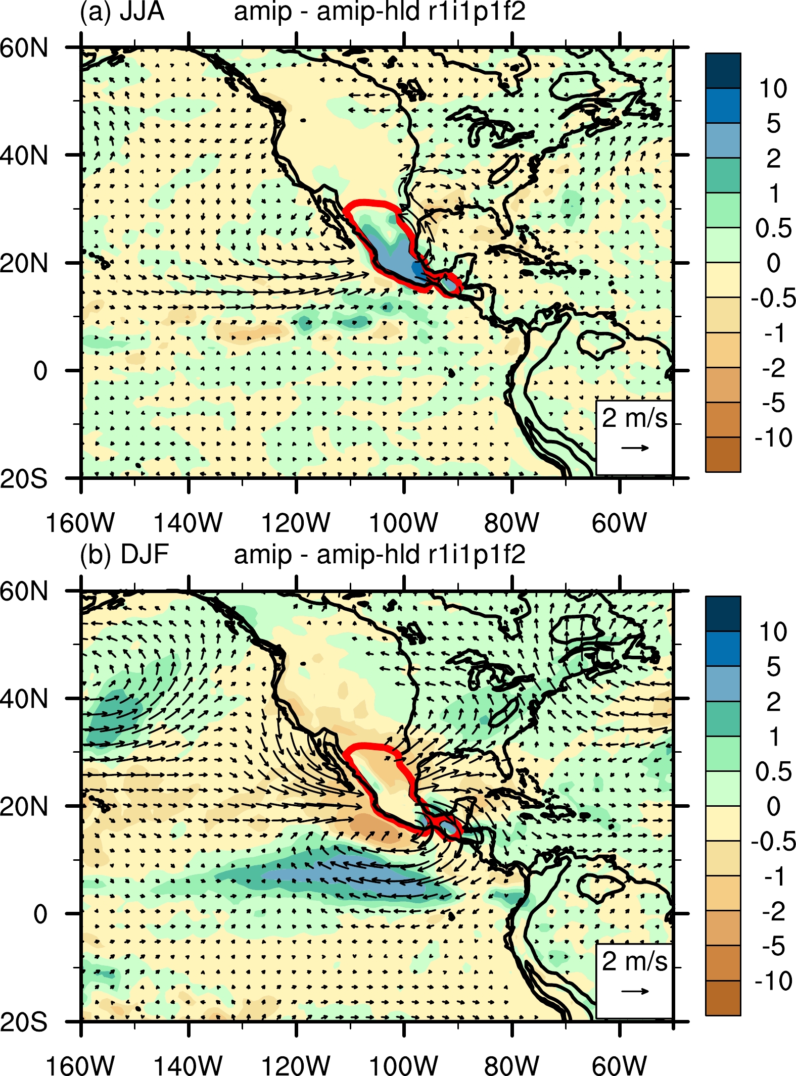 Figure8. (a) Climatological (1979–2014) JJA mean precipitation (shaded; units: mm d–1) and 850-hPa wind (vectors; units: m s?1) differences between amip r1i1p1f1 and amip-hld r1i1p1f2. (b) As in (a) but for the DJF mean. The red contour denotes the topography modified in amip-hld r1i1p1f2.
The Sierra Madre Mountains are important to the formation of the North American monsoon system (Adams and Comrie, 1997) and to the East Pacific typhoon activities (Zehnder, 1993). We show the JJA differences of precipitation and 850-hPa winds between amip r1i1p1f1 and amip-hld r1i1p1f2 in Fig. 8a. The orographic forcing of the Sierra Madres clearly generates a low-level cyclonic circulation anomaly and leads to increased local precipitation. This pattern is reasonable according to the thermal adaption theory proposed by Wu and Liu. (2000), which states that the orography acts as a heating forcing in the lower troposphere during the summertime. For DJF (Fig. 8b), the Sierra Madre induces a cyclonic circulation anomaly to its north and an anticyclonic circulation anomaly to its south, accompanied by a decreased precipitation anomaly surrounding the mountains and an increased precipitation anomaly mainly over the East Pacific and the eastern part of the North American continent.
The Andes Mountains are the dominant topographic feature in South America. Previous literature suggests that the Andes are critical to the formation of the South American low-level jet (Gandu and Geisler, 1991; Campetella and Vera, 2002), moisture transport, convection, and precipitation over South America (Insel et al., 2010; Junquas et al., 2016). In our experiments, we remove the Andes Mountains in amip-hld r1i1p1f3. The differences between amip r1i1p1f1 and amip-hld r1i1p1f3 are shown in Fig. 9. The JJA difference of the 850-hPa circulation (Fig. 9a) shows a cyclonic anomaly over subtropical South America and a strong westerly anomaly over the eastern tropical Pacific, accompanied by increased precipitation over the East Pacific around 10°N and along the meridionally oriented Andes. For DJF (Fig. 9b), the difference in the wind anomaly is quite close to the JJA pattern, while the difference in the precipitation anomaly shows an increase mainly over the southern part of South America and a decrease over the Amazon Basin, which is close to Fig. 4 in Junquas et al. (2016).
 Figure9. (a) Climatological (1979–2014) JJA mean precipitation (shaded; units: mm d–1) and 850-hPa wind (vectors; units: m s?1) differences between amip r1i1p1f1 and amip-hld r1i1p1f3. (b) As in (a) but for the DJF mean. The red contour denotes the topography modified in amip-hld r1i1p1f3.
Based on the above analysis, the basic performance of the CAS FGOALS-f3-L model in the GMMIP Tier-1 & Tier-3 experiments is justified. Finally, we show some more information on the output datasets. The output contains high temporal frequency (three-hourly mean, six-hourly snapshot and mean) datasets for the amip-TIP and amip-TIP-nosh experiments, which is beyond the requirement of GMMIP. The total size of the amip-TIP and amip-TIP-nosh experiments is approximately 2.5 TB each, and the total sizes of amip-hld r1i1p1f1, amip-hld r1i1p1f2 and amip-hld r1i1p1f3 are approximately 0.3 TB each. Detailed information on the output variables is also shown in Table 2 for reference.
| Output name | Description | Frequency (3-h mean, 6-h snapshot only for amip-TIP and amip-TIP-nosh) |
| rlut | TOA outgoing longwave radiation | Monthly |
| rsdt | TOA incident shortwave radiation | Monthly |
| rsut | TOA outgoing shortwave radiation | Monthly |
| rlutcs | TOA outgoing clear-sky longwave radiation | Monthly |
| rsutcs | TOA outgoing clear-sky shortwave radiation | Monthly |
| rlds | Surface downwelling longwave radiation | Monthly, 3 h |
| rlus | Surface upwelling longwave radiation | Monthly, 3 h |
| rsds | Surface downwelling shortwave radiation | Monthly, 3 h |
| rsus | Surface upwelling shortwave radiation | Monthly, 3 h |
| rldscs | Surface downwelling clear-sky longwave radiation | Monthly, 3 h |
| rsdscs | Surface downwelling clear-sky shortwave radiation | Monthly, 3 h |
| rsuscs | Surface upwelling clear-sky shortwave radiation | Monthly, 3 h |
| tauu | Surface downward eastward wind stress | Monthly |
| tauv | Surface downward northward wind stress | Monthly |
| hfss | Surface upward sensible heat flux | Monthly, 3 h |
| hfls | Surface upward latent heat flux | Monthly, 3 h |
| pr | Precipitation | Monthly, daily, 3 h |
| evspsbl | Evaporation | Monthly |
| ts | Surface skin temperature | Monthly |
| tas | Near-surface air temperature | Monthly, daily, 3 h |
| tasmax | Daily maximum near-surface air temperature | Monthly, daily |
| tasmin | Daily minimum near-surface air temperature | Monthly, daily |
| uas | Eastward near-surface wind | Monthly, 3 h |
| vas | Northward near-surface wind | Monthly, 3 h |
| sfcWind | Near-surface wind speed | Monthly |
| huss | Near-surface specific humidity | Monthly, daily, 3 h |
| hurs | Near-surface relative humidity | Monthly, daily |
| clt | Total cloud fraction | Monthly, 3 h |
| ps | Surface air pressure | Monthly, 3 h, 6 h |
| psl | Sea level pressure | Monthly, daily |
| snc | Snow area fraction | Monthly, 3 h |
| ta | Air temperature at model level | Monthly, 6 h |
| ua | Eastward wind at model level | Monthly, 6 h |
| va | Northward wind at model level | Monthly, 6 h |
| hus | Specific humidity at model level | Monthly, 6 h |
| hur | Relative humidity at model level | Monthly |
| zg | Geopotential height at model level | Monthly |
Table2. CAS FGOALS-f3-L output variables prepared for CMIP6 GMMIP experiments.
Acknowledgements. The research presented in this paper was funded by the National Natural Science Foundation of China (Grant Nos. 91737306, 91637312, 41730963, 91837101, 91637208, 41530426), and the Key Research Program of Frontier Sciences, Chinese Academy of Sciences (Grant QYZDY-SSW-DQC018).
Open Access This article is distributed under the terms of the Creative Commons Attribution License which permits any use, distribution, and reproduction in any medium, provided the original author(s) and the source are credited.
