Pei-Ying Xiong¹, Khurram Javid², Mohsin Raza², Sami Ullah Khan³, M Ijaz Khan⁴, Yu-Ming Chu^,51College of Science, Hunan City University, Yiyang 413000, China
²Department of Mathematics, Northern University, Wattar-Walai Ziarat, Kaka Saib Road, 24110, Nowshera, KPK, Pakistan
³Department of Mathematics, COMSATS University Islamabad, Sahiwal 57000, Pakistan
⁴Department of Mathematics and Statistics, Riphah International University I-14, Islamabad 44000, Pakistan
⁵Department of Mathematics, Huzhou University, Huzhou 313000, China

Received:2020-12-02Revised:2021-04-13Accepted:2021-04-29Online:2021-06-21


Abstract
The steady laminar flow of viscous fluid from a curved porous domain under a radial magnetic field is considered. The fluid flow by a curved domain is due to peristaltic waves present at the boundary walls. The whole analysis is based on porosity (Darcy number) effects. Moreover, the effects of second-order slip on the rheology analysis are also discussed. Due to the complex nature of the flow regime, we have governed the rheological equations by using curvilinear coordinates in the fixed frame. The physical influence of magnetic (Hartmann number) and porosity (Darcy number) parameters on the rheological features of peristaltic transportation are argued in detailed (in the wave frame). Additionally, in the current study, the complex wavy pattern on both boundary walls of the channel is used. The whole rheological study is based on ancient, but medically valid, assumptions of creeping phenomena and long wavelength assumptions. Analytical solutions of the governing equations are obtained by using the simple integration technique in Mathematica software 11.0. The core motivation of the present analysis is to perceive the physical influence of embedded parameters, such as the dimensionless radius of the curvature parameter, magnetic parameter, porosity parameter, different amplitude ratios of complex peristaltic waves, first- and second-order slip parameters, on the axial velocity, pressure gradient, local wall shear stress, tangential component of the extra-stress tensor, pumping and trapping phenomena.
Keywords： peristaltic waves;magnetic field;porous medium;pumping phenomena;second-order slip condition


PDF (4612KB)MetadataMetricsRelated articlesExportEndNote|Ris|BibtexFavorite
Cite this article
Pei-Ying Xiong, Khurram Javid, Mohsin Raza, Sami Ullah Khan, M Ijaz Khan, Yu-Ming Chu. MHD flow study of viscous fluid through a complex wavy curved surface due to bio-mimetic propulsion under porosity and second-order slip effects. Communications in Theoretical Physics, 2021, 73(8): 085001- doi:10.1088/1572-9494/abfcb2

Nomenclature
$A$half width of the channel
$a$the wave speed
$\bar{X}$the axial coordinate
$\bar{t}$time
${\bar{\in }}_{1},\,{\bar{\in }}_{2}$different wave amplitudes
${\bar{\alpha }}_{1},\,{\bar{\alpha }}_{2}$the wave parameters
$\lambda $the wave length
$\left(\bar{R},\bar{X},\bar{Z}\right)$the curvilinear coordinates
$\left(\bar{v},\,\bar{u}\right)$the velocity field in the wave frame
$\left(\bar{x},\,\bar{r}\right)$the curvilinear coordinates in the wave frame
${\rm{\Omega }}$the dimensionless radius of curvature
${D}{a}$Darcy number
${\tau }_{ij}$the dimensionless form of extra-stress tensor
$\bar{R}$the radial coordinate
$\bar{X}$the axial coordinate
$\bar{Z}$the flow component in the z-direction.
$\bar{V}$the radial velocity
$\bar{U}$the axial velocity
$\bar{E}$electric field
$\bar{M}$magnetic field
$\sigma $the fluid electrical conductivity
${R}{e}$the Reynolds number
$\delta $the wave number
${H}{a}$Hartmann number
$\left({{\epsilon }}_{1},{{\epsilon }}_{2}\right)$the dimensionless symbols of different amplitudes of complex peristaltic waves
$\left({\beta }_{1},{\beta }_{2}\right)$the first- and second-order slip parameters

1. Introduction

Peristaltic propulsion is a biological phenomenon in which the motion of physiological fluids takes place through physiological vessels and arteries due to the continuous contraction and relaxation of these small vessels and arteries, such as the movement of a small food bolus through the oesophagus, urine transportation through the ureter, the motion of blood through blood vessels, air and gas movement through small arteries of the lung system, the movement of food from the mouth to the stomach, transportation of bile in bile ducts, intestinal chyme movement, ovum movement in the fallopian tube, and other hollow tubes. In these phenomena, physiological fluids are moved from one part of the vessel where the pressure is higher to another part of the vessel where the pressure is smaller by a continuous process of muscle contraction and relaxation. The periodic transportations of these vessels are actuated due to electro–chemical responses occurring in the body. Many industrial pumps, such as micro-pumps, mini-pumps, handy-pumps, integrating filling systems, roller pumps, compact peristaltic pumps, and standard peristaltic pumps, are based on the peristaltic pumping phenomenon. Applications in engineering fluid mechanics utilize caustic fluid (atomic industries), destructive chemicals, high solid slurries and numerous materials which are transported by peristaltic pumps. In the mid 1960s, Latham [1] first studied the mathematical modelling of peristaltic pumping with a seminal study (both analytically and experimentally) on biomechanical pumping. Two years after Latham’s work [1], in 1968, Fung and Yih [2] theoretically performed the same study as Latham [1]. After these two studies, a new horizon was developed in the research community and researchers performed dynamic research in this domain. In 1969, Shapiro et al [3] studied the mathematical modelling of the peristaltic motion of a viscous fluid and verified the fundamental findings of Latham [1]. Their analysis is based upon bio assumptions and arguments over the reflux and trapping phenomena during peristalsis. In this era, some fundamental contributions were performed, as given in [4–6].

Many industrial instruments and systems, including smart lubrication systems [7], nanomaterial fabrication [8], biomimetic pumps [9], separation devices, and magnetic blood pumps [10], are based on the study of magneto-hydrodynamics (MHD) to control the flow system, to acquire the performance augmentation, material influence, etc. A massive range of phenomena emerges in flows, such as the Hall current, Ohmic dissipation, ferromagnetism, oscillation, Landau damping, and oscillation. The utilization of magnetic fields in electrically conducting streams are produced by Lorentz powers (Lorentz forces), which can control rheological features.

Over the past two decades, the mathematical formulations of the MHD flow of numerous fluids due to peristaltic phenomena have gained considerable attention. The magnetic force has diverse applications, especially in MRI, that is used nowadays in hospitals to control blood motion (haematological diseases) during complex surgeries. Tripathi and Beg [11] have studied the magnetic and porosity effects, respectively, on the peristaltic motion of couple stress bio-fluid through coaxial channels. Ali et al [12] discussed the peristaltic propulsion of Newtonian fluid through a two-dimensional channel with variable viscosity. Furthermore, they have argued the rheological features under the influence of magnetic field and slip effects in detail under bio assumptions. Hayat and Ali [13] have deliberated the rheological study of third grade fluid through a deformable tube under a magnetic field. They have obtained the analytical solution by using the perturbation technique. In another research study, Hayat and Ali [14] have discussed the rheological analysis related to the peristaltic transportation of a viscoelastic Jeffrey fluid through a tube with a sinusoidal wave travelling down its boundary walls. The whole rheological analysis is based on a uniform magnetic field. Further productive research studies in this area are given in [15–17].

The internal motion of physiological fluids through a confined porous channel with contraction and relaxation walls has significant applications in biological flows, for example, blood flow through blood vessels, artificial dialysis, and air circulation in the lung system. Further applications include pulsating diaphragms, cerebral hydrodynamics, oxygen diffusion in the capillaries, the mechanics of the cochlea in the human ear, filtration in tissue, and cosmetics material manufacturing. Hayat et al [18] have performed dynamic research and highlighted the influence of partial slip and porosity effects on the biomimetic motion of Newtonian fluid. They obtained the solution for the stream function and axial velocity analytically by using the Adomian decomposition method. Alsaedi et al [19] examined the transportation of an incompressible couple stress bio-fluid through a porous channel under creeping phenomena. They attained the exact solutions of a system of rheological equations. Hayat et al [20] have argued over the peristaltic flow of Maxwell fluid in a planar channel under uniform porosity and Hall effects, respectively. They modelled the governing equations with the help of modified Darcy law (MDL). An impressive amount of research in this regard has been performed by some researchers and cited in [21–23].

The motion of Maxwell fluid through a moving plate has been studied by Lin and Guo [24] under magnetic effects. They have considered the second-order slip between the walls and the fluid. An analytical solution of a system of rheological equations is acquired by using Laplace transformation. They also obtained the solution for the simple slip (first-order slip) condition. Aly and Ebaid [25] have performed a flow study which deals with the peristaltic motion of nanofluid through an asymmetric channel under the influence of second-order velocity slip. They have obtained the exact solutions of the flow equations in terms of the stream function. Many mathematicians have performed dynamic research concerning the simple slip, and the second-order slip is cited in [26–28].

To the best of our knowledge, in 2000, Sato et al [29] were the first to perform productive research by using the curved channel. They have discussed the motion of two-dimensional Newtonian fluid through a curved domain in the fixed frame. They obtained the rheological equations by using curvilinear coordinates because of the complex shape of flow geometry. After the productive research work of Sato et al [29], in 2008, Ali et al [30] prolonged the study of Sato et al [29] in the wave frame. They solved the Navier–Stokes equations analytically with the help of an integration technique. In these studies [29, 30], their main concern was to focus the sound effects of the curvature parameter on a Newtonian fluid flow. Their whole research studies are based on bio approximations, respectively. These two research studies generated a new method of research for mathematicians. Researchers performed good research studies by using the different nature of fluids through the curved channel under numerous physical effects, such as, magnetic effects, electric effects, porosity effects, complaint wall effects, electro–magneto–hydrodynamic effects, heat transfer effects, heat and mass transfer effects, etc, as fluid flows because of the sinusoidal contraction and relaxation of boundary walls. The physical influence of heat transfer on the peristaltic transportation of a viscous fluid through a curved domain has been studied by Ali et al [31]. They obtained the numerical solution by using the Runge–Kutta algorithm. They observed the effects of the curvature parameter (physical parameter related to flow geometry) and Brinkman number (the heat flux parameter) on numerous rheological features. They also provided a comparison between curved and straight channels. They noticed that the rate of heat transfer in the curved domain is smaller than the straighter channel. Tanveer et al [32] presented an investigation related to the numerical simulation for the transportation of a Carreau–Yasuda nanofluid model through a curved channel. They also discussed the porosity effects by using MDL. After these productive studies, some researchers [33–38] discussed the rheological characteristics of numerous fluids through curved geometries under the lubrication approach and bio assumption, respectively, where they highlighted the influence of various physical forces, such as electric forces, magnetic forces, electro–magneto–hydrodynamics forces, heat transfer effects and mass transfer effects by using the different nature of fluids that flow through the curved geometry. Their main intention was to highlight the physical influence of the curvature parameter on numerous rheological features. They solved the rheological equations both analytically (the integration method, perturbation technique, singular perturbation technique) and numerically (the shooting method, Runge–Kutta technique, finite difference technique, finite element technique, BVP4C (boundary value problem) technique).

To the best of our knowledge, no studies have so far been performed with regard to the peristaltic transport of a viscous fluid from a curved channel in porous medium. Complex sinusoidal waves are present at the boundary walls of the flow regime. The main objective of the present manuscript is therefore to scrutinize the influence of the dimensionless curvature parameter, porous media, second-order slip parameter and magnetic field on the rheological characteristics of Newtonian fluid under creeping phenomena. An analytical solution is developed with an integration technique in Mathematica software 11.0. This is the novelty of the current study.

2. Mathematical formulation

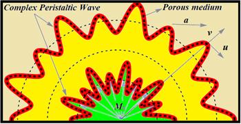
In the current study, we have considered a curved channel that is illustrated in figure 1. When the boundary walls of the curved channel are brought under the influence of peristaltic waves, initially, one section of the wall starts to contract at the inlet and the component positioned immediately ahead of this starts to relax, and this propagation of contraction and relaxation is continuous throughout the length of boundary walls. Finally, this propagation of the wave moves towards the outlet. This phenomenon continues until the whole transportation takes place. The fluid which is present inside the confined domains of the curved channel is initially at rest during the boundary walls when they are in a stationary state. But as the peristaltic waves are generated at the boundary walls, then fluid starts to move with the same speed and direction as the peristaltic waves. Additionally, the sinusoidal peristaltic wave existing at the boundary walls is complex in shape. This type of pattern is used to increase the efficiency and accuracy of roller and peristaltic pumps, respectively. For five years, this complex pattern of waves has been attracting the attention of researchers. Some dynamic research has been performed by various mathematicians and researchers by using the complex wavy pattern of peristaltic waves and obtaining productive outcomes that are mentioned in [39, 40]. Additionally, a radial magnetic field is applied to the rheostat of the fluid transportation.

Figure 1.

New window|Download| PPT slide
Figure 1.Flow geometry.


The mathematical expression of the complex peristaltic wave that propagates along the geometric walls is defined as:(1)$\begin{eqnarray}\begin{array}{l}\bar{H}\left(\bar{X},\,\bar{t}\right)=A+{\bar{\in }}_{1}\,\cos \left(\displaystyle \frac{{\bar{\alpha }}_{1}\pi }{\lambda }\left(\bar{X}-a\bar{t}\right)\right)\\ \,+{\bar{\in }}_{2}\,\cos \left(\displaystyle \frac{{\bar{\alpha }}_{2}\pi }{\lambda }\left(\bar{X}-a\bar{t}\right)\right)\,\left({\rm{Upper}}\,{\rm{wall}}\right)\end{array}\end{eqnarray}$(2)$\begin{eqnarray}\begin{array}{l}-\bar{H}\left(\bar{X},\,\bar{t}\right)=-A-{\bar{\in }}_{1}\,\cos \left(\displaystyle \frac{{\bar{\alpha }}_{1}\pi }{\lambda }\left(\bar{X}-a\bar{t}\right)\right)\\ \,-{\bar{\in }}_{2}\,\cos \left(\displaystyle \frac{{\bar{\alpha }}_{2}\pi }{\lambda }\left(\bar{X}-a\bar{t}\right)\right)\,\left({\rm{Lower}}\,{\rm{wall}}\right)\end{array}\end{eqnarray}$where $A$ is the half width of the channel, $a$ is the wave speed, $\bar{X}$ is the axial coordinate, $\bar{t}$ is time, ${\bar{\in }}_{1},\,{\bar{\in }}_{2}$ are different wave amplitudes, ${\bar{\alpha }}_{1},\,{\bar{\alpha }}_{2}$ are the wave parameters related to the amplitude of different waves and $\lambda $ is the wave length. The mandatory and abundant condition for complex peristaltic waves is $A\leqslant {\bar{\in }}_{1}\,+\,{\bar{\in }}_{2}.$ Due to the curved shape of the flow geometry, curvilinear coordinates are used to analyse the fluid flow. A coordinate (curvilinear coordinates) system is used in which coordinate lines may be curved in nature. This system of coordinates may be a result of introducing a linear relation from the Cartesian coordinates. Such coordinates generate a one-to-one map at each point. Mathematically, we obtained the required curvilinear coordinates from this linear transformation. Let us consider the curvilinear coordinates $\left(\bar{R},\bar{X},\bar{Z}\right)$ that are used in the present analysis, where $\bar{R}$ is the radial coordinate, $\bar{X}$ is the axial coordinate and $\bar{Z}$ is the flow component in the z-direction. Let us consider the velocity field $\left(\bar{V},\,\bar{U},0\right)$ for the two-dimensional flow rate, where $\bar{V}$ is the radial velocity, $\bar{U}$ is the axial velocity and there is no flow in the z-direction. There is no stream in the z-direction orthogonal to the $\bar{R}\bar{X}-{\rm{p}}{\rm{l}}{\rm{a}}{\rm{n}}{\rm{e}}.$

MHD is an outlet of applied physics that deals with the relation between the magnetic field and electrically conducting fluids, for example, electrolytes, liquid metals, magnetofluids, including plasmas and briny water. Physically, the essential thought behind MHD is that when the magnetic field is applied to a moving conductive fluid, then the fluid is polarized and, reciprocally, it deviates from the magnetic field. The external force exerted on a moving charge particle $Q$ with a velocity field $\bar{W}$ through both electric $\left(\bar{E}\right)$ and magnetic $(\bar{M})$ fields, respectively, is called the Lorentz force. The mathematical expression of the Lorentz force is defined below:(3)$\begin{eqnarray}\bar{F}=Q\bar{E}+\sigma \left(\bar{W}\times \bar{M}\right),\end{eqnarray}$where $\sigma $ is the fluid electrical conductivity. In the current manuscript, we will consider the weaker strength of an electric field, say $\bar{E}=0.$ Then, the above equation will reduce to the following form:(4)$\begin{eqnarray}\bar{F}=\sigma (\bar{W}\times \bar{M}).\end{eqnarray}$According to divergence law, the divergence of the magnetic field $\bar{M}=\left({M}_{r},{M}_{\theta },{M}_{z}\right)$ is zero, $\bar{{\rm{\nabla }}}\cdot \bar{M}=0,$ we acquire ${M}_{r}=\tfrac{{M}_{0}\bar{{\rm{\Omega }}}}{\bar{R}+\bar{{\rm{\Omega }}}}.$ Here, ${M}_{0}$ is the strength of the radial magnetic field, i.e., $\bar{M}=\left(\displaystyle \frac{{M}_{0}\bar{{\rm{\Omega }}}}{\bar{R}+\bar{{\rm{\Omega }}}},0,0\right)$ [37, 39](5)$\begin{eqnarray}\bar{W}\times \bar{M}=\left|\begin{array}{lll}{e}_{R} & {e}_{X} & {e}_{z}\\ \bar{V} & \bar{U} & 0\\ \displaystyle \frac{{M}_{0}\bar{{\rm{\Omega }}}}{\bar{R}+\bar{{\rm{\Omega }}}} & 0 & 0\end{array}\right|=-\left(\displaystyle \frac{{M}_{0}\bar{{\rm{\Omega }}}}{\bar{R}+\bar{{\rm{\Omega }}}}\right)\bar{U}{e}_{z}.\end{eqnarray}$Using equation (5) in (4), we get(6)$\begin{eqnarray}\bar{F}=-\left(\displaystyle \frac{\sigma \bar{U}{M}_{0}\bar{{\rm{\Omega }}}}{\bar{R}+\bar{{\rm{\Omega }}}}\right){e}_{z}.\end{eqnarray}$According to Maxwell law, we have(7)$\begin{eqnarray}\begin{array}{l}\bar{F}\times \bar{M}=\left|\begin{array}{lll}{e}_{R} & {e}_{X} & {e}_{z}\\ 0 & 0 & -\left(\displaystyle \frac{\sigma \bar{U}{M}_{0}\bar{{\rm{\Omega }}}}{\bar{R}+\bar{{\rm{\Omega }}}}\right)\\ \displaystyle \frac{{M}_{0}\bar{{\rm{\Omega }}}}{\bar{R}+\bar{{\rm{\Omega }}}} & 0 & 0\end{array}\right|\\ \,=-\sigma {\left(\displaystyle \frac{{M}_{0}\bar{{\rm{\Omega }}}}{\bar{R}+\bar{{\rm{\Omega }}}}\right)}^{2}\bar{U}{e}_{X}.\end{array}\end{eqnarray}$

The mathematical expression of the Cauchy-stress tensor $\left(\bar{T}\right)$ for a viscous fluid is defined as:(8)$\begin{eqnarray}\bar{T}=-P\bar{I}+\bar{S},\end{eqnarray}$where $P$ is the pressure term, $\bar{I}$ is the identity tensor, and $\bar{S}$ is the extra-stress tensor. The vector form of the extra-stress tensor for the Newtonian fluid model is defined as:(9)$\begin{eqnarray}\bar{S}=\mu \dot{Y}\end{eqnarray}$where $\dot{Y}$ is the shear stress, and $\mu $ is the dynamic viscosity.

Fluid mechanics has three fundamental equations: (i) continuity equation, (ii) momentum equation, and (iii) energy equation, respectively. These three dynamic equations provide the physics of dynamic systems. Their mathematical statement is based upon the three fundamental laws of physics: the law of conservation of mass, momentum and energy. These equations are expressed in a differential form of time and space coordinates, respectively.

The vector representations of rheological equations are:(10)$\begin{eqnarray}\bar{{\rm{\nabla }}}\cdot \bar{W}=0,\end{eqnarray}$(11)$\begin{eqnarray}\displaystyle \frac{D\bar{W}}{D\bar{t}}=-\displaystyle \frac{1}{\rho }\bar{{\rm{\nabla }}}P+\nu {{\rm{\nabla }}}^{2}\bar{W}+\displaystyle \frac{1}{\rho }\left(\bar{F}\times \bar{M}\right),\end{eqnarray}$where,(12)$\begin{eqnarray}\displaystyle \frac{D}{D\bar{t}}=\displaystyle \frac{\partial }{\partial \bar{t}}+\bar{W}\cdot \bar{{\rm{\nabla }}}\end{eqnarray}$(13)$\begin{eqnarray}\bar{W}\cdot \bar{{\rm{\nabla }}}=\displaystyle \frac{\bar{V}\bar{{\rm{\Omega }}}}{\bar{R}+\bar{{\rm{\Omega }}}}\displaystyle \frac{\partial }{\partial \bar{X}}+\bar{U}\displaystyle \frac{\partial }{\partial \bar{R}},\end{eqnarray}$(14)$\begin{eqnarray}{{\rm{\nabla }}}^{2}={\left(\displaystyle \frac{\bar{{\rm{\Omega }}}}{\bar{R}+\bar{{\rm{\Omega }}}}\right)}^{2}\displaystyle \frac{{\partial }^{2}}{\partial {\bar{X}}^{2}}+\left(\displaystyle \frac{1}{\bar{R}+\bar{{\rm{\Omega }}}}\right)\displaystyle \frac{\partial }{\partial \bar{R}}+\displaystyle \frac{{\partial }^{2}}{\partial {\bar{R}}^{2}}.\end{eqnarray}$The mathematical forms of the rheological equations in terms of curvilinear coordinates are expressed as:(15)$\begin{eqnarray}\displaystyle \frac{\partial }{\partial \bar{R}}\left(\left(\bar{R}+\bar{{\rm{\Omega }}}\right)\bar{V}\right)+\bar{{\rm{\Omega }}}\displaystyle \frac{\partial \bar{U}}{\partial \bar{X}}=0,\end{eqnarray}$(16)$\begin{eqnarray}\begin{array}{l}\displaystyle \frac{\partial \bar{V}}{\partial \bar{t}}+\bar{V}\displaystyle \frac{\partial \bar{V}}{\partial \bar{R}}+\left(\displaystyle \frac{\bar{U}\bar{{\rm{\Omega }}}}{\bar{R}+\bar{{\rm{\Omega }}}}\right)\displaystyle \frac{\partial \bar{V}}{\partial \bar{X}}-\displaystyle \frac{{\bar{U}}^{2}}{\bar{R}+\bar{{\rm{\Omega }}}}=-\displaystyle \frac{1}{\rho }\displaystyle \frac{\partial \bar{P}}{\partial \bar{R}}\\ \,+\displaystyle \frac{1}{\rho }\left(\displaystyle \frac{1}{\bar{R}+\bar{{\rm{\Omega }}}}\displaystyle \frac{\partial }{\partial \bar{R}}\left(\left(\bar{R}+\bar{{\rm{\Omega }}}\right){S}_{\bar{R}\bar{R}}\right)\right.\\ \,+\left.\left(\displaystyle \frac{\bar{{\rm{\Omega }}}}{\bar{R}+\bar{{\rm{\Omega }}}}\right)\displaystyle \frac{\partial {S}_{\bar{R}\bar{X}}}{\partial \bar{X}}-\displaystyle \frac{{S}_{\bar{X}\bar{X}}}{\bar{R}+\bar{{\rm{\Omega }}}}\right)-\displaystyle \frac{\upsilon }{K}\left(\displaystyle \frac{\bar{{\rm{\Omega }}}}{\bar{R}+\bar{{\rm{\Omega }}}}\right)\bar{V},\end{array}\end{eqnarray}$(17)$\begin{eqnarray}\begin{array}{l}\displaystyle \frac{\partial \bar{U}}{\partial \bar{t}}+\bar{V}\displaystyle \frac{\partial \bar{U}}{\partial \bar{R}}+\left(\displaystyle \frac{\bar{U}\bar{{\rm{\Omega }}}}{\bar{R}+\bar{{\rm{\Omega }}}}\right)\displaystyle \frac{\partial \bar{U}}{\partial \bar{X}}-\displaystyle \frac{\bar{U}\bar{V}}{\bar{R}+\bar{{\rm{\Omega }}}}\\ \,=-\displaystyle \frac{1}{\rho }\left(\displaystyle \frac{\bar{{\rm{\Omega }}}}{\bar{R}+\bar{{\rm{\Omega }}}}\right)\displaystyle \frac{\partial \bar{P}}{\partial \bar{X}}\\ \,+\displaystyle \frac{1}{\rho }\left(\displaystyle \frac{1}{{\left(\bar{R}+\bar{{\rm{\Omega }}}\right)}^{2}}\displaystyle \frac{\partial }{\partial \bar{R}}\left({\left(\bar{R}+\bar{{\rm{\Omega }}}\right)}^{2}{S}_{\bar{X}\bar{R}}\right)\right.\\ \,+\left.\left(\displaystyle \frac{\bar{{\rm{\Omega }}}}{\bar{R}+\bar{{\rm{\Omega }}}}\right)\displaystyle \frac{\partial {S}_{\bar{X}\bar{X}}}{\partial \bar{X}}\right)\\ \,-\,\displaystyle \frac{\sigma }{\rho }{\left(\displaystyle \frac{{M}_{0}\bar{{\rm{\Omega }}}}{\bar{R}+\bar{{\rm{\Omega }}}}\right)}^{2}\bar{U}-\displaystyle \frac{\upsilon }{K}\left(\displaystyle \frac{\bar{{\rm{\Omega }}}}{\bar{R}+\bar{{\rm{\Omega }}}}\right)\bar{U}.\end{array}\end{eqnarray}$In the above equations, the mathematical terms ${S}_{\bar{R}\bar{R}},\,{S}_{\bar{R}\bar{X}},\,{S}_{\bar{X}\bar{X}}$ are the components of the extra-stress tensor and $\upsilon $ is the dynamic viscosity. The dimensional form of the components of the extra-stress tensor are given below:(18a)$\begin{eqnarray}{S}_{\bar{X}\bar{X}}=2\mu \displaystyle \frac{\partial \bar{V}}{\partial \bar{R}},\end{eqnarray}$(18b)$\begin{eqnarray}{S}_{\bar{R}\bar{X}}=\mu \left(\displaystyle \frac{{\partial }^{2}\bar{U}}{\partial {\bar{R}}^{2}}+\left(\displaystyle \frac{\bar{{\rm{\Omega }}}}{\bar{R}+\bar{{\rm{\Omega }}}}\right)\displaystyle \frac{\partial \bar{V}}{\partial \bar{R}}+\displaystyle \frac{\bar{U}}{\bar{R}+\bar{{\rm{\Omega }}}}\right),\end{eqnarray}$(18c)$\begin{eqnarray}{S}_{\bar{R}\bar{R}}=2\mu \left(\left(\displaystyle \frac{\bar{{\rm{\Omega }}}}{\bar{R}+\bar{{\rm{\Omega }}}}\right)\displaystyle \frac{\partial \bar{U}}{\partial \bar{X}}+\displaystyle \frac{\bar{{\rm{V}}}}{\bar{R}+\bar{{\rm{\Omega }}}}\right).\end{eqnarray}$In this section, we will introduce a linear transformation between fixed and wave frames, respectively. The wave frame is moving with the wave speed ‘a’. The main cause of linear transformation is to shift the flow system from an unsteady state to a steady state. The mathematical expressions of these linear relations are defined as:(19)$\begin{eqnarray}\bar{x}=\bar{X}-a\bar{t},\,\bar{r}=\bar{R},\,\bar{v}=\bar{V},\,\bar{u}=\bar{U}-a,\,\,P=\bar{P}.\end{eqnarray}$Here, $\left(\bar{v},\,\bar{u}\right)$ is the velocity field and $\left(\bar{x},\,\bar{r}\right)$ are the curvilinear coordinates in the wave frame. After applying equation (19) in to the above system of equations (equations (15)–(18)), we obtained rheological equations in the wave frame.

The non-dimensional or dimensionless numbers and physical parameters are those which are significant in order to explain the numerous rheological features of fluids. These dimensionless numbers are a combination of numerous physical characteristics, such as force, density, speed, length parameter, etc. The Hartmann number (magnetic parameter) and Reynolds number are two famous dimensionless numbers. Another main advantage of these dimensionless numbers is that the quantity of the physical embedded variables is condensed.

Introducing the dimensionless variables:(20)$\begin{eqnarray}\begin{array}{l}x=\displaystyle \frac{2\pi \bar{x}}{\lambda },\,r=\displaystyle \frac{\bar{r}}{A},\,v=\displaystyle \frac{\bar{v}}{a},\,u=\displaystyle \frac{\bar{u}}{a},\,{R}{e}=\displaystyle \frac{\rho aA}{\mu },\,h=\displaystyle \frac{\bar{W}}{A},\,\\ \delta =\displaystyle \frac{2\pi A}{\lambda },\,{\rm{\Omega }}=\displaystyle \frac{\bar{{\boldsymbol{\Omega }}}}{A},\,{H}{a}=\sqrt{\displaystyle \frac{\sigma }{\mu }}{M}_{0}A,\,{D}{a}=\sqrt{\displaystyle \frac{K}{\nu }}\\ \alpha =\displaystyle \frac{a\overline{{\lambda }_{1}}}{A},\,\gamma =\displaystyle \frac{a\overline{{\lambda }_{2}}}{A},\,{{\epsilon }}_{1}=\displaystyle \frac{\overline{{{\epsilon }}_{1}}}{A},\,{{\epsilon }}_{2}=\displaystyle \frac{\overline{{{\epsilon }}_{2}}}{A},\,\,p=\displaystyle \frac{2\pi \bar{P}}{\lambda \mu A},\,\,\\ {\tau }_{ij}=\displaystyle \frac{A}{\mu a}{S}_{\bar{i}\bar{j}},\,\,{\beta }_{1}=\displaystyle \frac{\mu a}{A}{\bar{\beta }}_{1},\,\,{\beta }_{2}=\displaystyle \frac{\mu a}{{A}^{2}}{\bar{\beta }}_{2}.\end{array}\end{eqnarray}$The stream function is a scalar function. Mathematically, these scalar functions are expressed in terms of the derivatives of time and space coordinates, respectively. Each derivative term represents a velocity component orthogonal to any direction. These stream functions give information about the rotational or irrotational flow of a fluid. If a fluid satisfies Laplace’s equation, it is said to be an irrotational fluid:(21)$\begin{eqnarray}v=\delta \displaystyle \frac{{\rm{\Omega }}}{{\rm{\Omega }}+r}\displaystyle \frac{\partial \psi }{\partial x},\,u=-\displaystyle \frac{\partial \psi }{\partial r},\end{eqnarray}$where $x$ is the axial component of geometry, $r$ is the radial component of geometry, $v$ is the radial velocity, $u$ is the axial velocity, ${R}{e}$ is the Reynolds number, $h$ is the upper half of the regime, $\delta $ is the wave number, ${\rm{\Omega }}$ is the dimensionless radius of curvature, ${H}{a}$ is the dimensionless magnetic parameter (Hartmann number), ${D}{a}$ is the dimensionless porosity parameter (Darcy number), $\left(\alpha ,\gamma \right)$ are the physical parameters, $\left({{\epsilon }}_{1},{{\epsilon }}_{2}\right)$ are the dimensionless symbols of the different amplitudes of complex peristaltic waves, $P$ is the pressure term, ${\tau }_{ij}$ is the dimensionless form of extra-stress tensor, $\left({\beta }_{1},{\beta }_{2}\right)$ are the first- and second-order slip parameters, respectively. After using these dimensionless variables and stream functions, we apply bio assumptions into a system of equations in a wave frame. These assumptions are called low Reynolds numbers (where the viscous force is much larger than the inertial force, and mathematically it is denoted as ${R}{e}\to 0$) and long wavelength (where the wavelength of the sinusoidal waves is much larger than the half width of the channel, and mathematically it is denoted as $\lambda \gg A$) approximations. Then, we get(22)$\begin{eqnarray}\displaystyle \frac{\partial p}{\partial r}=0,\end{eqnarray}$(23)$\begin{eqnarray}\begin{array}{l}-\displaystyle \frac{\partial p}{\partial x}-\displaystyle \frac{1}{{\rm{\Omega }}\left({\rm{\Omega }}+r\right)}\displaystyle \frac{\partial }{\partial r}\left(\left({\rm{\Omega }}+r\right)\left(1-\displaystyle \frac{\partial \psi }{\partial r}\right)\right.\\ \,+\left.{\left({\rm{\Omega }}+r\right)}^{2}\displaystyle \frac{{\partial }^{2}\psi }{\partial {r}^{2}}\right)\\ \,-{\left(\displaystyle \frac{{H}{a}{\rm{\Omega }}}{{\rm{\Omega }}+r}\right)}^{2}\left(1-\displaystyle \frac{\partial \psi }{\partial r}\right)-\displaystyle \frac{1}{{{Da}}^{2}}{\left(\displaystyle \frac{{\rm{\Omega }}}{{\rm{\Omega }}+r}\right)}^{2}\\ \,\times \left(1-\displaystyle \frac{\partial \psi }{\partial r}\right)=0,.\end{array}\end{eqnarray}$It is obvious from equation (22) that the pressure term is independent of the radial coordinate. In equation (23), two dependent variables are present: one is the pressure term and the second is the stream function. In order to eliminate the pressure from equation (23) by using cross derivatives between equations (22) and (23), we obtain:(24)$\begin{eqnarray}\begin{array}{l}\displaystyle \frac{\partial }{\partial r}\left(\displaystyle \frac{1}{{\rm{\Omega }}\left({\rm{\Omega }}+r\right)}\displaystyle \frac{\partial }{\partial r}\left(\left({\rm{\Omega }}+r\right)\left(1-\displaystyle \frac{\partial \psi }{\partial r}\right)\right.\right.\\ \,+\left.{\left({\rm{\Omega }}+r\right)}^{2}\displaystyle \frac{{\partial }^{2}\psi }{\partial {r}^{2}}\right)\\ \left.\,+{\left(\displaystyle \frac{{H}{a}{\rm{\Omega }}}{{\rm{\Omega }}+r}\right)}^{2}\left(1-\displaystyle \frac{\partial \psi }{\partial r}\right)+\displaystyle \frac{1}{{{Da}}^{2}}{\left(\displaystyle \frac{{\rm{\Omega }}}{{\rm{\Omega }}+r}\right)}^{2}\right)\\ \,\times \left.\left(1-\displaystyle \frac{\partial \psi }{\partial r}\right)\right)=0,\end{array}\end{eqnarray}$An alternative form of equation (24) is(25)$\begin{eqnarray}\begin{array}{l}\displaystyle \frac{\partial }{\partial r}\left(\displaystyle \frac{1}{{\rm{\Omega }}\left({\rm{\Omega }}+r\right)}\displaystyle \frac{\partial }{\partial r}\left(\left({\rm{\Omega }}+r\right)\left(1-\displaystyle \frac{\partial \psi }{\partial r}\right)+{\left({\rm{\Omega }}+r\right)}^{2}\displaystyle \frac{{\partial }^{2}\psi }{\partial {r}^{2}}\right)\right.\\ \,\left.+\left({{Ha}}^{2}+\displaystyle \frac{1}{{{Da}}^{2}}\right){\left(\displaystyle \frac{{\rm{\Omega }}}{{\rm{\Omega }}+r}\right)}^{2}\left(1-\displaystyle \frac{\partial \psi }{\partial r}\right)\right)=0.\end{array}\end{eqnarray}$Let ${G}^{2}={\rm{H}}{{\rm{a}}}^{2}+\tfrac{1}{{\rm{D}}{{\rm{a}}}^{2}},$ then the above equation will be:(26)$\begin{eqnarray}\begin{array}{l}\displaystyle \frac{\partial }{\partial r}\left(\displaystyle \frac{1}{{\rm{\Omega }}\left({\rm{\Omega }}+r\right)}\displaystyle \frac{\partial }{\partial r}\left(\left({\rm{\Omega }}+r\right)\left(1-\displaystyle \frac{\partial \psi }{\partial r}\right)+{\left({\rm{\Omega }}+r\right)}^{2}\displaystyle \frac{{\partial }^{2}\psi }{\partial {r}^{2}}\right)\right.\\ \left.\,+{G}^{2}{\left(\displaystyle \frac{{\rm{\Omega }}}{{\rm{\Omega }}+r}\right)}^{2}\left(1-\displaystyle \frac{\partial \psi }{\partial r}\right)\right)=0.\end{array}\end{eqnarray}$Equation (26) is the required fourth order ODE that describes the rheological topographies of a Newtonian fluid by the curved geometry in terms of the stream function.

The second-order slip boundary conditions (see [24–28]) in terms of the stream function are:(27)$\begin{eqnarray}\psi =-\displaystyle \frac{F}{2},\,\,\displaystyle \frac{\partial \psi }{\partial r}=-{\beta }_{1}{\tau }_{rx}-{\beta }_{2}\displaystyle \frac{\partial }{\partial r}{\tau }_{rx}+1,\,\,{\rm{a}}{\rm{t}}\,r=h,\end{eqnarray}$(28)$\begin{eqnarray}\psi =\displaystyle \frac{F}{2},\,\,\displaystyle \frac{\partial \psi }{\partial r}=-{\beta }_{1}{\tau }_{rx}-{\beta }_{2}\displaystyle \frac{\partial }{\partial r}{\tau }_{rx}+1,\,\,{\rm{a}}{\rm{t}}\,r=-h,\end{eqnarray}$where F is the dimensionless flow rate, ${\beta }_{1}$ is the first-order slip parameter and ${\beta }_{2}$ is the second-order slip parameter.

The pressure rise can be expressed as the mathematical form defined as [30–35]:(29)$\begin{eqnarray}{\boldsymbol{\Delta }}P=\displaystyle {\int }_{0}^{1}\displaystyle \frac{{\rm{d}}p}{{\rm{d}}x}{\rm{d}}x.\end{eqnarray}$The mathematical term is related to the pressure gradient, which is present in the above equation (29) as ${\rm{d}}p/{\rm{d}}x.$ The pressure gradient defines the rate of change (derivative or slope) of the pressure term w.r.t the axial coordinate, while ${\boldsymbol{\Delta }}P$ is the pressure rise per wavelength in each cross-section.

The analytical solution of equation (26) is obtained by using an integration technique in the Mathematica software 11.0:(30)$\begin{eqnarray}\begin{array}{l}\psi =r+\displaystyle \frac{{\left({\rm{\Omega }}+r\right)}^{1+\sqrt{1+G{{\rm{\Omega }}}^{2}}}}{1+\sqrt{1+G{{\rm{\Omega }}}^{2}}}{A}_{1}+\displaystyle \frac{{\left({\rm{\Omega }}+r\right)}^{1-\sqrt{1+G{{\rm{\Omega }}}^{2}}}}{1-\sqrt{1+G{{\rm{\Omega }}}^{2}}}{A}_{2}\\ \,+\left({\rm{\Omega }}r+\displaystyle \frac{{r}^{2}}{2}\right){A}_{3}+{A}_{4}.\end{array}\end{eqnarray}$The axial velocity is obtained by taking the partial differential of equation (30) w.r.t r:(31)$\begin{eqnarray}\begin{array}{l}\displaystyle \frac{\partial \psi }{\partial r}=1+{\left({\rm{\Omega }}+r\right)}^{\sqrt{1+G{{\rm{\Omega }}}^{2}}}{A}_{1}+{\left({\rm{\Omega }}+r\right)}^{-\sqrt{1+G{{\rm{\Omega }}}^{2}}}{A}_{2}\\ \,+\left({\rm{\Omega }}+r\right){A}_{3}.\end{array}\end{eqnarray}$(32)$\begin{eqnarray}\begin{array}{l}u=-\displaystyle \frac{\partial \psi }{\partial r}=-1-{\left({\rm{\Omega }}+r\right)}^{\sqrt{1+G{{\rm{\Omega }}}^{2}}}{A}_{1}\\ \,-{\left({\rm{\Omega }}+r\right)}^{-\sqrt{1+G{{\rm{\Omega }}}^{2}}}{A}_{2}-\left({\rm{\Omega }}+r\right){A}_{3},\end{array}\end{eqnarray}$where ${A}_{i}\,(i=1-4)$ are the constant of integrations. These constants can be obtained by utilizing Mathematica software 11.0.

The local wall shear stress at the upper wall of the channel is:(33)$\begin{eqnarray}\tau ={\left.\displaystyle \frac{\partial u}{\partial r}\right|}_{r=h}.\end{eqnarray}$Taking partial differential of equation (32) w.r.t r:(34)$\begin{eqnarray}\begin{array}{l}\displaystyle \frac{\partial u}{\partial r}=-\sqrt{1+G{{\rm{\Omega }}}^{2}}{\left({\rm{\Omega }}+r\right)}^{-1-\sqrt{1+G{{\rm{\Omega }}}^{2}}}{A}_{1}\\ \,+\sqrt{1+G{{\rm{\Omega }}}^{2}}{\left({\rm{\Omega }}+r\right)}^{-1+\sqrt{1+G{{\rm{\Omega }}}^{2}}}{A}_{2}-{A}_{3}\end{array}\end{eqnarray}$at $r=h$(35)$\begin{eqnarray}\begin{array}{l}\tau =-\sqrt{1+G{{\rm{\Omega }}}^{2}}{\left({\rm{\Omega }}+h\right)}^{-1-\sqrt{1+G{{\rm{\Omega }}}^{2}}}{A}_{1}\\ \,+\sqrt{1+G{{\rm{\Omega }}}^{2}}{\left({\rm{\Omega }}+h\right)}^{-1+\sqrt{1+G{{\rm{\Omega }}}^{2}}}{A}_{2}-{A}_{3}.\end{array}\end{eqnarray}$Special Case:

The rheological results of [30] are retrieved by neglecting the magnetic effects, porosity effects and complex wavy scenario of peristaltic waves from the rheological equations.

All these results give authenticity to the correctness and validation of obtaining governing equations. The range of physical parameters are given in table 1.


Table 1.
Table 1.Range of physical parameters.

Physical parameter	Range	Physical parameter	Range
${\beta }_{1}$	[0, 5]	$\in 1$	$0.3$
${\beta }_{2}$	[0, 5]	$\in 2$	$0.4$
${H}{a}$	[0, 100]	${\rm{\Omega }}$	$3.5$
${D}{a}$	[0, $\infty $)	$A$	$1$

New window|CSV

3. Graphical consequences and interpretations

The transport problem amounts to a 4th-order system of linear and ODE defined by equations (22)–(23) with BC’s in equations (27) and (28). This BVP is solved analytically using the four-time integration in Mathematica. Validation of the current flow analysis has been conducted with existing results in the literature. The results of [30] are acquired by eliminating some physical flow features.

In this section, we shall examine the physical influence of involved parameters such as the curvature parameter ${\rm{\Omega }},$ different amplitude ratios of complex peristaltic waves $\left({{\epsilon }}_{1},{{\epsilon }}_{2}\right),$ the Hartmann number ${H}{a},$ Darcy number ${D}{a},$ first- and second-order slip parameters $\left({\beta }_{1},{\beta }_{2}\right)$ on the axial velocity, pressure gradient, pumping phenomena, extra shear stress tensor, the local shear stress at the upper walls, and trapping phenomena, respectively with the help of graphical illustration. Figures 2–4 illustrate selected flow distributions of the physical variables, which is, axial velocity, pressure gradient, pressure rise, component of the extra stress tensor, local shear stress, and trapping phenomena with radial and axial coordinates, respectively.

Figure 2.

New window|Download| PPT slide
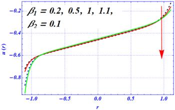
Figure 2.The variation of the velocity profile for the first-order slip parameter $({\beta }_{1})$ at ${\rm{\Omega }}=3.5,\,\in 1=0.3,\,\in 2=0.4,\,x=\pi ,\,A=1,{H}{a}=1,\,{D}{a}=0.1,\,Q=1.$

Figure 3.

New window|Download| PPT slide
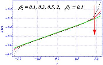
Figure 3.The variation of the velocity profile for the first-order slip parameter $\left({\beta }_{2}\right)$ at ${\rm{\Omega }}=3.5,\in 1=0.3,\in 2=0.4,x=\pi ,A=1,{H}{a}=1,{D}{a}=0.1,Q=1.$

Figure 4.

New window|Download| PPT slide
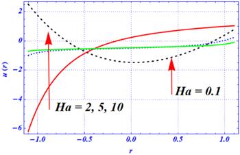
Figure 4.The variation of the velocity profile for the magnetic parameter $({H}{a})$ at ${\rm{\Omega }}=3.5,\,\in 1=0.3,\,\,\in 2=0.4,\,\,{\beta }_{1}=0.01\,{\beta }_{2}\,=0.1\,x=\pi ,\,A=1,\,{D}{a}=50,\,\,Q=1.$

3.1. Axial velocity profile

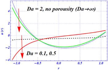
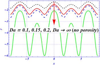
Figures 2–5 show the impacts of the Hartmann number ${H}{a},$ Darcy number ${D}{a},$ first- and second-order slip parameters $\left({\beta }_{1},{\beta }_{2}\right),$ i.e., with the radial coordinate. The magnitude of the axial velocity of Newtonian fluid through a curve is decreased by increasing the length of both slip parameters (see figures 2 and 3). These results are obtained under the influence of two external forces: one is the magnetic force and the other is the porous medium. The difference between these two figures is that the magnitude of the axial velocity sharply decreases by enhancing the second-order slip parameter from 0.1 to 2 and fixing the first-order slip parameter, say ${\beta }_{1}=0.1.$ Physically, these two results show that the magnitude of the velocity profile at both the walls is larger in the absence of both slip parameters as compared with the non-zero values of the slip parameters. Figure 4 depicts the impact of the Hartmann number on the velocity profile under larger porosity effects. At smaller strengths of magnetic field, say Ha=0.1, the magnitude of the velocity profile is larger. But as the numeric value of the Hartmann number changes from 0.1 to 2, not only is the magnitude of the velocity profile larger but it also shifts from the lower half to the upper half of the channel. Additionally, when the magnetic strength is enhanced from 2 to 10, then the magnetic effects are dominant over the porosity effects and the magnitude of the velocity profile reduces. These results show that a larger strength of magnetic field has a dynamic impact on the velocity profile and sharp changes are predicted under a larger magnetic strength. Here, the magnetic effects are dominant over the curvature effects. The physical influence of the Darcy number on the axial velocity is displayed in figure 5 under the larger strength of the magnetic field. Here, we have noticed two distinct results for smaller and larger values of the Darcy number. When Da changes from 0.1 to 0.5, then the amplitude of the axial velocity is enhanced near the boundary walls of the curved channel. Just like the previous result of Ha, it is also observed that the velocity profile shifts toward the lower half of the curved channel as the numeric value of Da changes from 0.5 to 2. Here, it can be noticed that the magnitude of the velocity profile is decreased at the lower half as Da increases from 2 to $\infty $ (no porosity). Physically, it means that under larger porosity effects, the magnitude of the velocity profile is smaller as compared with the weaker strength of the porosity effects.

Figure 5.

New window|Download| PPT slide
Figure 5.The variation of the velocity profile for the porosity parameter $\left({D}{a}\right)$ at ${\rm{\Omega }}=3.5,\,\in 1=0.3,\,\,\in 2=0.4,\,{\beta }_{1}=0.01,{\beta }_{2}=0.1\,x=\pi ,\,A=1,\,{H}{a}=1,\,Q=1.$

3.2. Pressure gradient

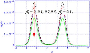
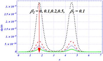
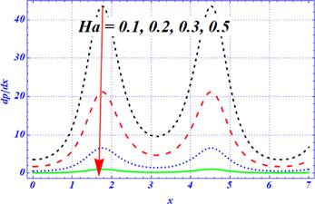
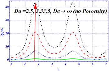
An important rheological characteristic of peristaltic motion that is concerned with the rate of change of the pressure function along the axial direction is called the pressure gradient. The impacts of the Hartmann number ${H}{a},$ Darcy number ${D}{a},$ first- and second-order slip parameters $\left({\beta }_{1},{\beta }_{2}\right),$ i.e., with the axial coordinate, are visualized in figures 6–9. Due to the complex nature of peristaltic waves, the wavy behavior is predicted in the graphs of the pressure gradient at each flow rate. In this subsection, the physical impacts of the physical parameters on the pressure gradient are highlighted under magnetic, curvature, porosity, Hartmann number, first- and second-order slip effects, respectively. The effects of a simple slip parameter under both larger curvature and porosity effects are displayed in figure 6. According to the literature survey, slip parameters reduce the magnitude of the pressure gradient. A comparative kind of conduct is anticipated in figure 6. As the numeric value of ${\beta }_{1}$ is enhanced, the magnitude of the pressure gradient is reduced under larger porosity effects. Physically, the larger values of the first-order slip parameter are dominant over the curvature and porosity effects which is why the magnitude of the pressure gradient is reduced. Figure 7 deals with the effects of the second-order slip parameter on the pressure gradient under curvature, porosity and magnetic effects, respectively. Once again, the magnitude of the pressure gradient is reduced as the length of the second-order slip parameter is increased. Physically, the larger values of the second-order slip parameter are dominant over the curvature and porosity effects which is why the magnitude of the pressure gradient is reduced. Furthermore, it is perceived that the magnitude of the pressure gradient sharply decreases in figure 7 by enhancing the length of ${\beta }_{2}$ as compared with the results of figure 6. The physical effects of porosity (Darcy number) and magnetic (Hartmann number) parameters on the pressure gradient are plotted in figures 8 and 9, respectively. According to the available literature, the magnetic force plays a role in reducing the magnitude of the pressure gradient. Similar results are obtained in figure 8; the magnitude of the pressure gradient is strongly affected by increasing the magnetic force, while the opposite is obtained in figure 9. The magnitude of the pressure gradient is enhanced as the Darcy number is increased. Physically, it means that under larger porosity effects or smaller values of Darcy number, the magnitude of the pressure gradient is smaller, while the reverse pattern is obtained for smaller porosity effects. Furthermore, it is noted that under the larger strength of both magnetic and porosity parameters, the magnitude of the pressure gradient is smaller as compared with the weaker strength of the magnetic and porosity effects.

Figure 6.

New window|Download| PPT slide
Figure 6.The variation of pressure gradient for the first-order slip parameter $({\beta }_{1})$ at ${\rm{\Omega }}=2,\,\,\in 1=0.3,\,\,\in 2=0.4,\,\,A=1,\,{H}{a}=1,{D}{a}=0.1,\,\,Q=1.$

Figure 7.

New window|Download| PPT slide
Figure 7.The variation of pressure gradient for the second-order slip parameter $\left({\beta }_{2}\right)$ at ${\rm{\Omega }}=2,\,\,\in 1=0.3,\,\in 2=0.4,\,A=1,{H}{a}=1,{D}{a}=0.1,\,\,Q=1.$

Figure 8.

New window|Download| PPT slide
Figure 8.The variation of pressure gradient for the Hartmann number $\left({Ha}\right)$ at ${\rm{\Omega }}=2,\,{\beta }_{1}={\beta }_{2}=0.1,\in 1=0.3,\,\in 2=0.4,A=1,\,{D}{a}=50,\,Q=1.$

Figure 9.

New window|Download| PPT slide
Figure 9.The variation of pressure gradient for the Darcy number $\left({D}{a}\right)$ at ${\rm{\Omega }}=2,\,{\beta }_{1}={\beta }_{2}=0.1,\in 1=0.3,\,\in 2=0.4,\,A=1,{H}{a}=1,\,Q=1.$

3.3. Pumping phenomena

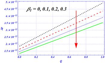
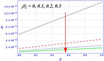
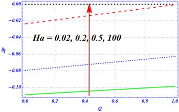
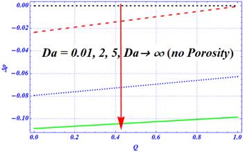
An important rheological phenomena related to peristalsis is known as the pumping phenomena. The mathematical definition of these phenomena is integrated with the pressure gradient term across a wavelength at each cross-sectional area. Graphically, a linear relation (graph) is obtained between the pressure rise and dimensionless flow rate parameter. The physical effects of the involved parameters, such as the dimensionless radius of curvature ${\rm{\Omega }},$ different amplitude ratios of complex peristaltic waves $\left({\epsilon }1,{\epsilon }2\right),$ Hartmann number ${H}{a},$ Darcy number ${D}{a},$ first- and second-order slip parameters $\left({\beta }_{1},{\beta }_{2}\right),$ on the pumping phenomena are visualized in figures 10–13. The effects of ${\beta }_{1}$ (first-order slip parameter) on the pumping phenomena are plotted in figure 10 for the complex peristaltic transportation of viscous fluid through a curved channel. In the absence of the first-order slip parameter, the magnitude of the pressure rise over the flow rate is maximum as compared with the presence of ${\beta }_{1}$ under porosity, magnetic and curvature effects. The magnitude of the pressure rise decreases by enhancing the first-order slip parameter from 0 to 0.3. A comparative kind of conduct is anticipated in figure 11 as observed in figure 10 for various values of the second-order slip parameter. Once again, the magnitude of the pressure rise decreases by enhancing the length of ${\beta }_{2}$ from 0 to 0.3. The main difference between these two figures is that the rate of change in the pumping phenomena is larger in figure 11 (for ${\beta }_{2}$) as compared with the outcomes of figure 10 (for ${\beta }_{1}$). Physically, the outcomes of both figures show that the slip effects overcome the magnetic and porosity effects. Furthermore, it is said that the pumping phenomena can be controlled with the help of the slip parameter. The magnetic effects are displayed in figure 12 on the pumping phenomena. In the absence of the Hartmann number, say ${H}{a}\,=\,0,$ the porosity and curvature effects are dominant. Due to these effects, the pressure rise is larger in magnitude for a viscous fluid. When the numeric value of the Hartmann number is increased from 0 to 100, then the magnitude of the rise in pressure is sharply reduced. Physically, the larger values of the magnetic field overcome the curvature and porosity effects, respectively. The physical effects of the porosity parameter are visualized in figure 13 on the pumping phenomena for the complex peristaltic motion of a viscous fluid under curvature, slip and magnetic effects, respectively. In this figure, we have observed the reverse behavior by enhancing the numeric values of the porosity parameter. For the smaller values of the Darcy number (when the effects of the porosity medium on the pumping phenomena are larger), the pressure rise has a smaller magnitude. Physically, the porosity effects are dominant over the curvature and magnetic effects. As ${D}{a}$ increases from 0 to $\infty ,$ the magnitude of the pumping phenomena is enhanced because of the weaker effects of the porous medium under larger curvature and magnetic effects. Additionally, the larger strength of the magnetic field and porosity medium play a dynamic role in the reduction of peristaltic pumping under curvature effects.

Figure 10.

New window|Download| PPT slide
Figure 10.The variation of pressure rise for the first-order slip parameter $\left({\beta }_{1}\right)$ at ${\rm{\Omega }}=2,\,\in 1=0.3,\,\in 2=0.4,\,A=1,{\beta }_{2}=0.1,{H}{a}=1,\,{D}{a}=0.1.$

Figure 11.

New window|Download| PPT slide
Figure 11.The variation of pressure rise for the second-order slip parameter $\left({\beta }_{2}\right)$ at ${\rm{\Omega }}=2,\,\in 1=0.3,\,\in 2=0.4,A=1,\,{H}{a}=1,{\beta }_{1}=0.1,\,{D}{a}=0.1.$

Figure 12.

New window|Download| PPT slide
Figure 12.The variation of pressure rise for the Hartmann number $\left({H}{a}\right)$ at ${\rm{\Omega }}=2,\in 1=0.3,\in 2=0.4,A=1,{\beta }_{1}={\beta }_{2}=0.1,{D}{a}=0.1.$

Figure 13.

New window|Download| PPT slide
Figure 13.The variation of pressure rise for the Hartmann number $\left({D}{a}\right)$ at ${\rm{\Omega }}=2,\,\in 1=0.3,\,\in 2=0.4,\,A=1,\,{\beta }_{1}={\beta }_{2}=0.1,{H}{a}=1.$

3.4. Shearing stress tensor

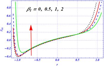
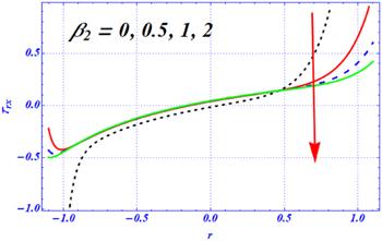
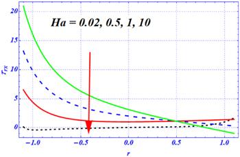
In this subsection, the graphs of the shearing component of the stress tensor are plotted through figures 14–17. The shearing stress tensor is also known as the tangential stress tensor. Figures 14–17 display the variation of the shearing stress tensor for different values of the Hartmann number ${H}{a},$ Darcy number ${D}{a},$ and first- and second-order slip parameters $\left({\beta }_{1},{\beta }_{2}\right).$ The magnitude of the shearing stress tensor at both walls is decreased by increasing the first-order slip (figure 14) effects for the biomimetic transportation of a viscous fluid under curvature, porosity and magnetic effects, respectively. Figure 15 is concerned with the effects of the second-order slip parameter on the shear stress of a viscous fluid. The magnitude of the shear stress tensor at both boundary walls is reduced by enhancing the length of the second-order slip parameter $\left({\beta }_{2}\right).$ Physically, in both figures 14 and 15, the magnitude of the shearing stress tensor sharply reduces by enhancing the strength of both slip parameters. The magnetic effects are visualized in figure 16 on the shearing stress tensor. The magnitude of the shearing stress tensor is larger in the absence of a magnetic field in the presence of both porosity and curvature effects, respectively. It is noticed that the magnitude of the shearing stress is reduced by increasing the magnetic force at larger numeric values of the Hartmann number. The boundary layer phenomena is observed for larger magnetic effects. The physical influence of the porous medium is displayed in figure 17 on the shear stress tensor. Here, the reverse behavior is predicted for the larger Darcy number. The magnitude of the shearing stress is increased at both the boundary walls by increasing the Darcy number. Additionally, the boundary layer phenomena is observed near the boundary walls for a smaller Darcy number. Physically, these two figures show that the larger strength of the magnetic field and porous medium play a dynamic role in producing the boundary layer phenomena immediate to the boundary walls. Additionally, these two forces play a dynamic role in controlling the behavior of the shearing stress tensor and larger values of both parameters overcome the curvature effects.

Figure 14.

New window|Download| PPT slide
Figure 14.The variation of the shearing stress tensor for the first-order slip parameter $\left({\beta }_{1}\right)$ at ${\rm{\Omega }}=3.5,{\beta }_{2}=0.1,A=1,{H}{a}=1,x=\pi ,Q=1,{D}{a}=0.1.$

Figure 15.

New window|Download| PPT slide
Figure 15.The variation of the shearing stress tensor for the second-order slip parameter $\left({\beta }_{2}\right)$ at ${\rm{\Omega }}=3.5,\,A={H}{a}=Q=1,\,{\beta }_{1}=0.1,x=\,\pi ,\,{D}{a}=0.1.$

Figure 16.

New window|Download| PPT slide
Figure 16.The variation of the shearing stress tensor for the magnetic parameter $\left({H}{a}\right)$ at ${\rm{\Omega }}=2,\,A=1,\,{\beta }_{1}={\beta }_{2}=0.1,x=\pi ,Q=1,\,{D}{a}=50.$

Figure 17.

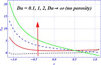New window|Download| PPT slide
Figure 17.The variation of the shearing stress tensor for the porosity parameter $\left({D}{a}\right)$ at ${\rm{\Omega }}=3.5,\,A=Q=1,\,x=\,\pi ,{\beta }_{1}={\beta }_{2}=0.1,{H}{a}=1.$

3.5. Local wall shear stress

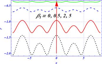
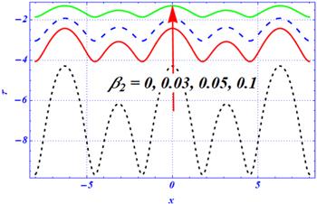
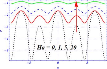
The variation of local shear stress at the upper wall of the curved channel is depicted in figures 18–21 with a variation of embedded physical parameters. The shape of its graph is the same as the shape of the peristaltic waves present at the upper wall of the channel. It is clear that the wavy graph is predicted because of the complex nature of the peristaltic waves. The components of the first- and second-order slip parameters are displayed in figures 18 and 19 for a viscous fluid. In the absence of slip parameters, the magnitude of local shear stress is maximum. When the length of the slip parameters is increased, then the magnitude of local shear stress is strongly affected. Because of this, the magnitude of the local shear stress decreases as the length of the slip parameters is increased. Physically, in both figures 18 and 19, the magnitude of the wall shear stress is sharply reduced by enhancing the strength of both slip parameters. The effects of magnetic force on the local shear stress under stronger porosity effects are depicted in figure 20 for the peristaltic flow of viscous fluid through a curved domain. In the absence of a magnetic parameter, the magnitude of local shear stress is larger. The magnitude of local shear stress is decreased by enhancing the magnetic effects. The magnitude of local shear stress is increased by increasing the Darcy number (figure 21). These results are in contrast to the magnetic effects. Additionally, in the presence of a smaller Darcy number, the effects of the porous medium are stronger, and due to this, the magnitude of local shear stress is reduced. Physically, under larger magnetic and porosity effects, the magnitude of local shear stress is strongly affected because these two external forces overcome the curvature effects. Further, these two figures (figures 20 and 21) show that the larger strength of the magnetic field and porous medium play a dynamic role in disturbing the sinusoidal behavior of wall shear stress under curvature effects. Additionally, these two forces play a dynamic role in controlling the behavior of wall shear stress and the larger values of both physical parameters overcome the curvature effects.

Figure 18.

New window|Download| PPT slide
Figure 18.The variation of local wall shear stress for the first-order slip parameter $\left({\beta }_{1}\right)$ at ${\rm{\Omega }}=3.5,{\beta }_{2}=0.1,A=1,{H}{a}=1,x=\pi ,{D}{a}=0.1.$

Figure 19.

New window|Download| PPT slide
Figure 19.The variation of local wall shear stress for the second-order slip parameter $\left({\beta }_{2}\right)$ at ${\rm{\Omega }}=3.5,A=1,{H}{a}=1,{\beta }_{1}=0.1,x=\pi ,{D}{a}=0.1.$

Figure 20.

New window|Download| PPT slide
Figure 20.The variation of local wall shear stress for the magnetic parameter $\left({H}{a}\right)$ at ${\rm{\Omega }}=3.5,A=1,{\beta }_{1}=0.01,Q=1,{\beta }_{2}=0.1,{D}{a}=1.$

Figure 21.

New window|Download| PPT slide
Figure 21.The variation of local wall shear stress for the porosity parameter $\left({D}{a}\right)$ at ${\rm{\Omega }}=3.5,A=1,{\beta }_{1}=0.01,Q=1,{\beta }_{2}=0.1,{H}{a}=1.$

3.6. Trapping phenomena

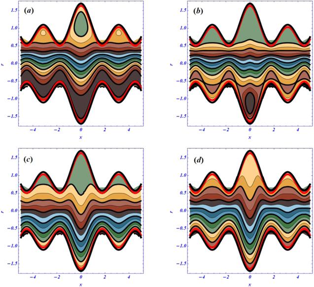
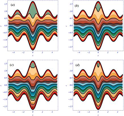
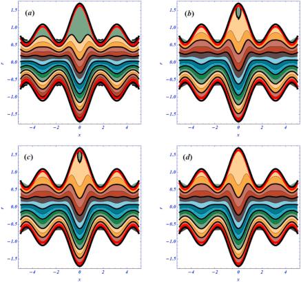
Another important rheological phenomena related to peristalsis is known as the trapping phenomena. This phenomenon is concerned with the bolus dynamics near the boundary walls. The shape of the bolus is the same as the shape of the peristaltic walls. The bolus is moved with the same speed and direction as the peristaltic waves. The influence of flow parameters on the trapping phenomena is visualized in figures 22–25. The effects of the magnetic parameter (Hartmann number) on the trapping phenomena under curvature, porosity and second-order slip effects are plotted in figure 22. We have noticed these results under larger porosity effects. In the absence of a magnetic field and the curved nature of the flow regime, the circulation of the bolus is present at the upper half of the channel under porosity effects. When the magnetic strength is increased by increasing the numeric values of the Hartmann number from 0 to 1, the circulation of the bolus is shifted to the lower half (figure 22(b)). As was our expectation, the circulation of the bolus disappears from both halves by increasing the Hartmann number from 5 to 50. Additionally, it is noticed that not only does the circulation of the bolus disappear, but the number of the streamlines is reduced too at a larger strength of the magnetic field. The effects of the porous medium are visualized in figure 23 under the curvature, second-order slip parameter and magnetic effects. Here, we have obtained the reverse behavior as compared with the results of figure 22. Under smaller porosity effects, the circulation of the bolus exists at the upper half of the regime at smaller porosity when ${D}{a}\to \,\infty .$ The circulation of the bolus is disturbed by enhancing the physical effects of the porous medium (see figures 23(c) and (d)). Physically, the larger strength of both external forces, the magnetic force and porous medium, on the trapping phenomena have sound effects to reduce the circulation of the bolus and number of streamlines form both halves of the channel. The effects of the second-order slip condition on the trapping phenomena are displayed in figures 24 and 25 under curvature, magnetic and porosity effects, respectively. According to the literature survey, the slip parameter plays a dynamic role in effecting the circulation of the bolus and streamlines. Here, the streamlines are present at the lower half of the channel due to the curvature and porosity effects. As the length of the slip parameters are increased, the number of the streamlines are reduced at both halves of the channel. Due to the complex nature of biomimetic waves, the wavy behavior in both the streamlines and trapping phenomena can be observed. Additionally, these results are obtained under larger curvature effects.

Figure 22.

New window|Download| PPT slide
Figure 22.(a)–(d). The variation of streamlines for ${H}{a}\,\left(0,\,1,\,5,\,50\right)$ at ${\rm{\Omega }}=3.5,\,A=1,\,{\beta }_{1}={\beta }_{2}=0.1,\,Q=1,\,{D}{a}=50.$

Figure 23.

New window|Download| PPT slide
Figure 23.(a)–(d). The variation of streamlines for ${D}{a}\,\left(\infty ,\,1,\,0.2,\,0.02\right)$ at ${\rm{\Omega }}=3.5,\,A=1,\,{\beta }_{1}={\beta }_{2}=0.1,\,Q=1,\,{H}{a}=\mathrm{0.02.}$

Figure 24.

New window|Download| PPT slide
Figure 24.(a)–(d): The variation of streamlines for ${\beta }_{1}\left(0,\,1,2,5\right)$ at ${\rm{\Omega }}=3.5,\,A=1,\,{\beta }_{2}=0.1,\,Q=1,\,\,{D}{a}=0.1,{H}{a}=0.1.$

Figure 25.

New window|Download| PPT slide
Figure 25.(a)–(d): The variation of streamlines for ${\beta }_{2}\,(0,0.5,2,5)$ at ${\rm{\Omega }}=3.5,\,A=1,\,{\beta }_{1}=0.1,\,Q=1,\,{D}{a}=0.1,{H}{a}=0.1.$

4. Conclusions

A mathematical study has been presented for the laminar and incompressible flow of Newtonian fluid through a curved domain with peristaltic waves at the boundary walls with a complex scenario. Due to the curved shape of flow geometry, curvilinear coordinates are used to govern the rheological equations. These equations have been non-dimensionalized by using similarity transformations. The integration technique has been used to solve the boundary value problem (BVP). The effects of curvature, magnetic, porosity and slip parameters on the axial velocity, pressure gradient, shear component of the stress tensor, pressure rise, local wall shear stress and trapping phenomena have been presented graphically and discussed in detail. The mathematical formulation which is relevant to the peristaltic pumping of a viscous fluid through the curved nature of flow geometry has shown that:

In axial velocity, the magnitude of the velocity profile is reduced near the boundary walls by increasing the length of the slip parameters. The magnitude of velocity is reduced for larger magnetic and porosity effects. The amplitude of the pressure gradient is reduced sharply as the slip parameters are enhanced under larger porosity effects. The larger strength of the magnetic field and porous medium reduced the magnitude of the pressure gradient for a viscous fluid. The magnitude of the pressure rise related to the peristaltic flow of Newtonian fluid through a curved domain is reduced linearly by increasing the slip effects and amplitude ratios of peristaltic waves. The larger strength of the magnetic field and porosity medium have a dynamic influence on reducing the pumping phenomena. The magnitude of the pressure gradient is reduced (increased) at larger values of the Hartmann number (Darcy number). The magnitude of the shearing stress tensor is reduced by increasing the length of the slip parameters. The boundary layer phenomena is obtained for larger magnetic and porosity effects, respectively. The magnitude of local wall shear stress is reduced by increasing the length of the slip parameters under porosity and curvature effects, respectively. Under the larger strength of magnetic and porous medium effects, the amplitude of local wall shear stress is reduced. The circulation of the bolus disappeared under larger magnitude of the magnetic and porosity forces, respectively, in the upper half of the channel. Under larger magnetic effects, a larger number of streamlines are present at the lower half of the channel due to the curved nature of the geometry. The circulation of the bolus appears at the upper half of the straight channel under larger magnetic effects. While no circulation of the bolus is present under larger porosity effects, the number of streamlines are larger at the lower half for the curved channel. The number of streamlines is reduced by increasing the length of both slip parameters.

In the current manuscript, the combined effects of magnetic field, porosity and second-order slip parameters on the peristaltic propulsion of viscous fluid through a curved regime are discussed. The main reason for performing this study is to understand the transportation of biological fluids through a curved channel. This study shows that the curved shape of the channel has dynamic effects on the transport phenomena of physiological fluids. Additionally, the role of the magnetic field on the moving fluid is more useful in the curative domain to control the motion of biological fluids through curved vessels. Furthermore, the porosity effects on transportation phenomena are utilized in chemical engineering. The role of complex sinusoidal waves on the boundary walls is utilized to boost the pumping phenomena. Ultimately, the second-order slip has sound impacts on the rheological features of bio fluids. This investigation can be extended to non-Newtonian liquids. This investigation gives information about the movement of biological fluids through complex peristaltic pumps under a larger porosity medium for engineers and scientists. Additionally, these effects are observed in the presence of the wavy nature of peristaltic propulsion. These are the novelties of the current study. This rheological analysis has various applications in medical, chemical and petroleum engineering domains for the manufacturing of micro-scale devices that are useful in medical therapy, blood pumping, drug delivery systems, chemical cooling systems and geophysics, respectively. Some recent contributions in this domain are cited in [41–48].

Reference View Option By original order
By published year
By cited within times
By Impact factor

[1]Latham T W 1966 Fluid motion in a peristaltic pump
MS Thesis MIT, Cambridge, AMA
[Cited within: 4]

[2]Yin F Fung Y C 1969 Peristaltic Waves in Circular Cylindrical Tubes 36 579 587
DOI:10.1115/1.3564720 [Cited within: 1]

[3]Shapiro A H Jaffrin M Y Weinberg S L 1969 Peristaltic pumping with long wavelength at low Reynolds number
J. Fluid Mech. 37 799 813
DOI:10.1017/S0022112069000899 [Cited within: 1]

[4]Burns J C Parkes T 1967 Peristaltic motion
J. Fluid Mech. 29 731 743
DOI:10.1017/S0022112067001156 [Cited within: 1]

[5]Yin F C P Fung Y C 1971 Comparison of theory and experiment in peristaltic transport
J. Fluid Mech. 47 93 112
DOI:10.1017/S0022112071000958

[6]Jaffrin M Y Shapiro A H 1971 Peristaltic pumping
Ann. Rev. Fluid Mech. 3 13 37
DOI:10.1146/annurev.fl.03.010171.000305 [Cited within: 1]

[7]Huang W Wang X 2016 Ferrofluids lubrication: a status report
Lubr. Sci. 28 3 26
DOI:10.1002/ls.1291 [Cited within: 1]

[8]Saima G Khan S B Rehman I U Khan M A Khan M I 2019 A comprehensive review of magnetic nanomaterials modern day theranostics
Frontiers Mater. 6 179
DOI:10.3389/fmats.2019.00179 [Cited within: 1]

[9]Bach D Schmich F Masselter T Speck T 2015 A review of selected pumping systems in nature and engineering—potential biomimetic concepts for improving displacement pumps and pulsation damping
Bioinsp. Biomim. 10 051001
DOI:10.1088/1748-3190/10/5/051001 [Cited within: 1]

[10]Mitamura Y Arioka S Sakota D Sekine K Azegami M 2008 Application of a magnetic fluid seal to rotary blood pumps
J. Phys.: Condens. Matter 20 204145
DOI:10.1088/0953-8984/20/20/204145 [Cited within: 1]

[11]Tripathi D Bég O A 2012 Magnetohydrodynamic peristaltic flow of a couple stress fluid through coaxial channels containing a porous medium
J. Mech. Med. Biol. 12 1250088
DOI:10.1142/S0219519412500881 [Cited within: 1]

[12]Ali N Hussain Q Hayat T Asghar S 2008 Slip effects on the peristaltic transport of MHD fluid with variable viscosity
Phys. Lett. A 372 1477 1489
DOI:10.1016/j.physleta.2007.09.061 [Cited within: 1]

[13]Hayat T Ali N 2006 Peristaltically induced motion of a MHD third grade fluid in a deformable tube
Physica A 370 225 239
DOI:10.1016/j.physa.2006.02.029 [Cited within: 1]

[14]Hayat T Ali N 2008 Peristaltic motion of a Jeffrey fluid under the effect of a magnetic field in a tube
Commun. Nonlinear Sci. Numer. Simul. 13 1343 1352
DOI:10.1016/j.cnsns.2006.12.009 [Cited within: 1]

[15]Hayat T Ali N Asghar S 2007 An analysis of peristaltic transport for flow of a Jeffrey fluid
Acta Mech. 193 101 112
DOI:10.1007/s00707-007-0468-2 [Cited within: 1]

[16]Abd-Alla A M Abo-Dahab S M Kilicman A 2015 Peristaltic flow of a Jeffrey fluid under the effect of radially varying magnetic field in a tube with endoscope
J. Magn. Magn. Mater. 384 79 86
DOI:10.1016/j.jmmm.2015.02.017

[17]Bég O A Rashidi M M 2013 Multi-step DTM simulation of magneto-peristaltic flow of a conducting Williamson viscoelastic fluid
Int. J. Appl. Math. Mech. 9 22 40
[Cited within: 1]

[18]Hayat T Hussain Q Ali N 2008 Influence of partial slip on the peristaltic flow in a porous medium
Physica A 387 3399 3409
DOI:10.1016/j.physa.2008.02.040 [Cited within: 1]

[19]Alsaedi A Ali N Tripathi D Hayat T 2014 Peristaltic flow of couple stress fluid through uniform porous medium
Appl. Math. Mech. 35 469 480
DOI:10.1007/s10483-014-1805-8 [Cited within: 1]

[20]Hayat T Ali N Asghar S 2007 Hall effects on peristaltic flow of a Maxwell fluid in a porous medium
Phys. Lett. A 363 397 403
DOI:10.1016/j.physleta.2006.10.104 [Cited within: 1]

[21]Guo X Zhou J Xie H Jiang Z 2018 MHD peristaltic flow of fractional Jeffrey model through porous medium
Math. Probl. Eng. 2018
DOI:10.1155/2018/6014082 [Cited within: 1]

[22]Lakshminarayana P Vajravelu K Sucharitha G Sreenadh S 2018 Peristaltic slip flow of a Bingham fluid in an inclined porous conduit with Joule heating
Appl. Math. Nonlinear Sci. 3 6014082
DOI:10.21042/AMNS.2018.1.00005

[23]Afifi N A S Gad N S 2003 Interaction of peristaltic flow with pulsatile fluid through a porous medium
Appl. Math. Comput. 142 167 176
DOI:10.1016/S0096-3003(02)00291-6 [Cited within: 1]

[24]Liu Y Guo B 2017 Effects of second-order slip on the flow of a fractional Maxwell MHD fluid
J. Assoc. Arab Univ. Basic Appl. Sci. 24 232 241
DOI:10.1016/j.jaubas.2017.04.001 [Cited within: 2]

[25]Aly E H Ebaid A 2014 Effect of the velocity second slip boundary condition on the peristaltic flow of nanofluids in an asymmetric channel: exact solution
Abstr. Appl. Anal. 2014 191876
DOI:10.1155/2014/191876 [Cited within: 1]

[26]Zhu J Yang D Zheng L Zhang X 2016 Effects of second order velocity slip and nanoparticles migration on flow of Buongiorno nanofluid
Appl. Math. Lett. 52 183 191
DOI:10.1016/j.aml.2015.09.003 [Cited within: 1]

[27]Hamdan M A Al-Nimr M A Hammoudeh V A 2010 Effect of second order velocity-slip/temperature-jump on basic gaseous fluctuating micro- flows
J. Fluids Eng. 132 074503
DOI:10.1115/1.4001970

[28]Sravanthi C S 2020 Second order velocity slip and thermal jump of Cu–water nanofluid over a cone in the presence of nonlinear radiation and nonuniform heat source/sink using homotopy analysis method
Heat Transfer—Asian Res. 49 86 102
DOI:10.1002/htj.21600 [Cited within: 2]

[29]Sato H Kawai T Fujita T Okabe M 2000 Two dimensional peristaltic flow in curved channels
Trans. Japan Soc. Mech. Eng. B 66 679 685
DOI:10.1299/kikaib.66.679 [Cited within: 4]

[30]Ali N Sajid M Hayat T 2010 Long wavelength flow analysis in a curved channel
Zeitschrift fur Naturforschung A 65a 191 196
DOI:10.1515/zna-2010-0306 [Cited within: 5]

[31]Ali N Sajid M Abbas Z Javed T 2010 Non-Newtonian fluid flow induced by peristaltic waves in a curved channel
Eur. J. Mech. B 29 387 394
DOI:10.1016/j.euromechflu.2010.04.002 [Cited within: 1]

[32]Anum T Hayat T Alsaedi A Ahmad B 2017 Numerical simulation for peristalsis of Carreau-Yasuda nanofluid in curved channel with mixed convection and porous space
PLoS One 12 e0170029
DOI:10.1371/journal.pone.0170029 [Cited within: 1]

[33]Hayat T Ahmed B Abbasi F M Alsaedi A 2019 Peristalsis of nanofluid through curved channel with Hall and Ohmic heating effects
J. Cent. South Univ. 26 2543 2553
DOI:10.1007/s11771-019-4193-5 [Cited within: 1]

[34]Ali N Javid K Sajid M Beg O A 2016 Numerical simulation of peristaltic flow of a biorheological fluid with shear-dependent viscosity in a curved channel
Comput. Methods BioMech. BioMed. Eng. 19 614 627
DOI:10.1080/10255842.2015.1055257

[35]Ali N Javid K Sajid M Zaman A Hayat T 2016 Numerical simulations of Oldroyd 8-constant fluid flow and heat transfer in a curved channel
Int. J. Heat and Mass Transfer 94 500 508
DOI:10.1016/j.ijheatmasstransfer.2015.11.066 [Cited within: 1]

[36]Ali N Sajid M Javid K Ahmed R 2017 Peristaltic flow of Rabinowitsch fluid in a curved channel: mathematical analysis revisited
Z. Naturforsch. A 72 245 251
DOI:10.1515/zna-2016-0334

[37]Khurram J Ali N Asghar Z 2019 Rheological and magnetic effects on a fluid flow in a curved channel with different peristaltic wave profiles
J. Braz. Soc. Mech. Sci. Eng. 41 483
DOI:10.1007/s40430-019-1993-3 [Cited within: 1]

[38]Fidelis O N Asghar S Charreh D 2020 Magnetohydrodynamic flow through a wavy curved channel
AIP Adv. 10 035114
DOI:10.1063/1.5142214 [Cited within: 1]

[39]Khurram J Ali N Asghar Z 2019 Numerical simulation of the peristaltic motion of a viscous fluid through a complex wavy non-uniform channel with magnetohydrodynamic effects
Phys. Scr. 94 115226
DOI:10.1088/1402-4896/ab2efb [Cited within: 2]

[40]Khurram J Khan S U-D Hassan M Saeed U Rizvi S T R Khan S U-D 2019 Peristaltic transportation of tluid through simple and complex wavy non-uniform channels: a bio-engineering application
Int. J Multiscale Comp. Eng. 17 623 638
[Cited within: 1]

[41]Gowda R P Kumar R N Aldalbahi A Issakhov A Prasannakumara B C Rahimi-Gorji M Rahaman M 2020 Thermophoretic particle deposition in time-dependent flow of hybrid nanofluid over rotating and vertically upward/downward moving disk
Surf. Interfaces 22 100864
DOI:10.1016/j.surfin.2020.100864 [Cited within: 1]

[42]Roja A Gireesha B J Prasannakumara B C 2020 MHD micropolar nanofluid flow through an inclined channel with entropy generation subjected to radiative heat flux, viscous dissipation and multiple slip effects
Multidiscipline Modeling Mater. Struct. 16 1475 1496
DOI:10.1108/MMMS-12-2019-0235

[43]Gireesha B J Shankaralingappa B M Prasannakumar B C Nagaraja B 2020 MHD flow and melting heat transfer of dusty Casson fluid over a stretching sheet with Cattaneo–Christov heat flux model
Int. J. Ambient Energy 1 9
DOI:10.1080/01430750.2020.1785938

[44]Sajjad H Ijaz N Zeeshan A Li Y-Z 2020 Magneto-hydrodynamics of a solid-liquid two-phase fluid in rotating channel due to peristaltic wavy movement
Int. J. Numer. Methods Heat Fluid Flow 30 2501 2516
DOI:10.1108/HFF-02-2019-0131

[45]Nouman I Riaz A Zeeshan A Ellahi R Sait S M 2020 Buoyancy driven flow with gas-liquid coatings of peristaltic bubbly flow in elastic walls
Coatings 10 115
DOI:10.3390/coatings10020115

[46]Hanan A Riaz A Razaq A Saleem N Zeeshan A Bhatti M M 2020 Effects of double diffusion convection on third grade nanofluid through a curved compliant peristaltic channel
Coatings 10 154
DOI:10.3390/coatings10020154

[47]Riaz A Zeeshan A Bhatti M M Ellahi R 2020 Peristaltic propulsion of Jeffrey nano-liquid and heat transfer through a symmetrical duct with moving walls in a porous medium
Physica A 545 123788
DOI:10.1016/j.physa.2019.123788

[48]Zeeshan A Bhatti M M Muhammad T Zhang L 2020 Magnetized peristaltic particle–fluid propulsion with Hall and ion slip effects through a permeable channel
Physica A 550 123999
DOI:10.1016/j.physa.2019.123999 [Cited within: 1]