 ,3, Muhammad Imran2, Malik Zaka Ullah41Department of Mathematics,
 2Department of Mathematics,
3Department of Mathematics, College of Sciences,
4Department of Mathematics, Faculty of Science,
Received:2020-01-04Revised:2020-06-01Accepted:2020-06-02Online:2020-09-16

Abstract
KeywordsЃК
PDF (1516KB)MetadataMetricsRelated articlesExportEndNote|Ris|BibtexFavorite
Cite this article
Sami Ullah Khan, Hassan Waqas, Taseer Muhammad, Muhammad Imran, Malik Zaka Ullah. Significance of activation energy and Wu's slip features in Cross nanofluid with motile microorganisms. Communications in Theoretical Physics, 2020, 72(10): 105001- doi:10.1088/1572-9494/aba250
Nomenclature
${K}_{n}$ Knudsen number${\alpha }^{* }$ momentum accommodation coefficient
${\beta }^{* }$ molecular mean free path
${K}_{1}$ combine parameter
n power law index parameter
$f$ velocity distribution
$\gamma $ first order slip factor
$\delta $ second order slip factor'
h heat transfer coefficient
$\phi $ nanoparticle concentration
$\beta $ time constant
$\varphi $ porous medium
${\rho }_{p}$ nanoparticle density
${\rho }_{m}$ density of motile microorganism
${\alpha }_{m}$ thermal diffusivity
${\left(\rho c\right)}_{f}$ fluid heat capacity
${D}_{T}$ thermodiffusion constant
$\kappa $ Boltzmann constant
${E}_{a}$ activation energy
${W}_{e}$ speed of cells
$\lambda $ mixed convection parameter
$We$ Weissenberg parameter
$Nr$ buoyancy ratio parameter
$Bi$ Biot parameter
$Le$ Lewis number
$Nb$ Brownian motion parameter
$Rd$ radiation parameter
$Pe$ Peclet number
${q}_{w}$ heat flux
${q}_{j}$ mass flux
$\tilde{N}{u}_{x},$ local Nusselt number
$\sigma * $ electrical conductivity
$k* $ porous medium permeability
$g$ gravity
$\tilde{T}$ nanoparticle temperature
$\tilde{C}$ nanoparticle concentration
${\left(\rho c\right)}_{p}$ nanoparticles' effective heat capacity
${D}_{B}$ diffusion constant
$Kr$ reaction constant
${b}_{1}$ chemotaxis constant
$Ha$ combined parameter
${\rm{\Gamma }}$ unsteady parameter
$Nc$ bioconvection Rayleigh number
$Pr$ Prandtl number
${\theta }_{w}$ temperature ratio parameter
$Nt$ thermophoresis parameter
$E$ activation energy parameter
${{\rm{\Omega }}}_{1}$ bioconvection constant
$Lb$ bioconvection Lewis number
${q}_{m}$ density flux
$S{h}_{x}$ local Sherwood number
$\tilde{N}{h}_{x}$ local density number
1. Introduction
Due to the rapid commercial, engineering and industrial significance of nanofluids, a fundamental interest has been developed by numerous researchers in recent days. The nanoparticles, a complex mixture of nano-sized particles (1-100 nm), attained highly improved thermo-physical features. Due to excellent enhanced resistance and miscellaneous characteristics, nanoparticles are efficiently used in mechanical, industrial, chemical and biological sciences such as cooling of various electronic chips, thermal reactors, chemical processes, fission reactions, sensor technology, catalysis, diagnoses and treatment of cancer tissue, brain tumors, antibacterial applications and many more. The fundamental applications of nanoparticles in thermal extrusion systems also overcome the attention of poor energy reservoirs. From the literature surveyed, it is noted that basic investigation on nanofluids was proposed by Choi [1]. This involuntary idea insisted scientists perform further interesting contributions in the flow of nanofluids in the presence of some unique flow features. For instance, Sheikholeslami et al [2] studied the forced convection flow of nanoparticles subjected to a magnetic field by utilizing the Lattice Boltzmann technique. Khan et al [3] analyzed the wedge flow of a Carreau nanofluid with the existence of heat absorption and generation features by employing the shooting technique. The combined heat and mass transportations based on modified Cattaneo-Christov theories in the flow of viscoelastic nanoparticles over a moving geometry was scrutinized by Hayat et al [4]. Mahanthesh et al [5] analyzed the mixed convective flow over a rotating frame with evaluation of Hall current effects. Siddiqui and Turkyilmazoglu [6] initiated an interesting contribution based on the flow of ferro-nanoparticles in a cavity. Hsiao [7] performed a theoretical model based on the flow of micropolar nanoparticles in the presence of viscous dissipation characteristics over a moving surface. The flow of rate type nanoliquid with a heat source and sink features over a rotating disk has been thrashed out numerically by Ahmed et al [8]. The study of graphene-water nanoparticles over a stretching/shrinking surface subject to suction and injection characteristics was examined by Aly [9]. The stability analysis for each critical value was determined and various results have been reported graphically. Rout and Mishra [10] performed a comparative study regarding magnetized nanoparticles over a moving surface. The interaction of SA-Al2O3 and SA-Cu nanoparticles with chemical reaction effects and slip features was reported by Tlili et al [11]. Hayat et al [12] studied a second grade nanofluid in two parallel disks where magnetic field effects were proposed perpendicularly. Khan and Shehzad [13] captured the Brownian motion and thermophoresis features in a third grade nanofluid over an accelerated surface. The flow of Maxwell viscoelasticity-based nanoparticles in the presence of slip consequences was specified numerically by Waqas et al [14]. Sheikholeslami et al [15] investigated the forced convective flow of a nanofluid in a three-dimensional enclosure in the presence of a hot cubic obstacle. Shehzad et al [16] explored both the magnetic field and porous medium effects on the flow of a micropolar nanofluid configured by a stretched surface. The study of Cross magneto-nanofluid in stagnation point flow of a contracting and expanding cylinder has been recently presented by Ali et al [17]. Li et al [18] evaluated the characteristics of nanoparticles in a storage finned in the presence of melting heat transfer.It is commonly observed that when microorganisms gathered near the upper surface of a fluid, the phenomenon of unstable density stratification appeared, which causes bioconvection. The variation in microorganisms is self propelled and due to the swimming of such microorganisms, some precise direction in the base fluid results in an enhanced base liquid density. During this process the microorganisms migrated towards the lower region due to density difference. The microorganisms are classified as gyrotaxis, gravitaxis and oxytaxis organisms. An interesting conflict between microorganisms and nanoparticles is justified as microorganisms are being self propelled while nanoparticles' movement is driven due to Brownian and thermophoresis features. The utilization of microorganisms in the nanoparticles can efficiently improve the suspension stability. The first continuation of the involvement of microorganisms in nanoparticles was presented by Kuznetsov [19]. Later on some inspired contributions have been reported by numerous researchers with various flow features. Alsaedi et al [20] inspected the bioconvection phenomenon with the utilization of nanoparticles over a moving configuration. The constituted problem was treated analytically via a homotopic algorithm. Alwatban et al [21] analyzed the features of bioconvection in a flow of Eyring Powell nanoparticles in the presence of an activation energy.
The anisotropic slip flow in the presence of Stefan blowing features and microorganisms over a rotating cone was numerically executed by Zohra et al [22]. Waqas et al [23] examined the phenomenon of motile microorganisms in nanomaterials over a porous surface. The flow of Sisko nanomaterials with second order slip effects and gyrotactic microorganisms was conducted by Farooq et al [24]. For numerical computation a famous finite difference approach was utilized with excellent accuracy. Khan et al [25] performed analysis dealing with the bioconvection flow of nanofluids. The boundary layer flow over a thin needle in a non-Newtonian nanofluid with motile microorganisms subject to the Stefan blowing consequences was determined by Amirsom et al [26]. The role of chemical reactions and energy activations in various fields of science oil emulsions, mechanical engineering, nuclear reactor cooling, chemical processes, and thermal reservoirs is quite necessitated. The activation energy is the amount of energy required to undergo the reaction processes. The basic work on this topic was initiated by Svante Arrhenius, which has been extended by much further research [27-31].
Due to the attractive response of bioconvection flow of nanofluids, the aim here is to examine the rheological consequences of a non-Newtonian nanofluid containing microorganisms in the presence of nonlinear thermal radiation and activation energy. A famous Cross fluid is utilized to examine the viscoelastic behavior [32, 33]. The main motivation of the present analysis is to report the bioconvection phenomenon in a flow of Cross nanofluid, which encountered some diverse and unique rheological characteristics. Moreover, this investigation has been executed by introducing the slip effects of second order. The utilization of a magnetized Cross nanofluid, thermal radiation, activation energy, gyrotactic microorganism and second order slip make this analysis quite versatile and motivating. The consideration of second order slip is more realistic, which involves two slip factors to control the thickness of the associated boundary layer. The formulated flow problem is numerically treated by using the shooting algorithm. A detailed graphically-based investigation for each flow parameter has been reported with relevant physical consequences.
2. Mathematical formulation
The unsteady and two-dimensional flow of a Cross nanoliquid over a stretched configuration has been examined with utilization of nonlinear thermal radiation and motile microorganisms. The considered flow has been assumed in the xy-plane where the velocity component u is taken in the x-direction and v is considered along the y-axis. A time-dependent magnetic force has been employed in the perpendicular direction where the influence of induced magnetic force is ignored with low Reynolds' number approximations. A well-known Buongiorno's nanoliquid model is incorporated to visualize the important consequences of Brownian movement and thermophoresis features. Additionally, the second order slip constraints (Wu's slip) are used near the stretched flow geometry. The transportation of combined heat and mass are controlled via a convective boundary and zero nanoparticles' mass flux constraints. The flow equations modeled on such assumptions may be expressed as [32, 33]:The second order slip boundary constraints (Wu's slip) for the flow problem are [34-37]:
By interaction of the above variables, we obtained the following set of dimensionless equations:
The transformed boundary assumptions are
The mathematical formulations for the local Nusselt number, local Sherwood number and motile density number are as follows:
In dimensionless forms, we have
3. Numerical approach
In order to determine the numerical computations for current dimensionless flow equations, we used a famous shooting technique to simulate the solution. We comprise the system of dimensionless flow equations from the boundary value problem to initial value problem as follows:Similarly the boundary conditions are transformed as
4. Discussion
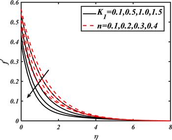
This section scrutinizes the graphical impact of various emerging parameters on the distribution of velocity, temperature, concentration and motile microorganisms. Each graph is plotted by assigning some constant values while the remaining physical parameters attained constant values such as ${K}_{1}=0.5,$ $We=1.0,$ $n=0.3,$ ${\rm{\Gamma }}=0.2,$ $Nc=0.2,$ $\gamma =1.0,$ $\delta =-1.0,$ $Pr=0.7,Nt=0.3,$ $Nb=0.2,$ ${\theta }_{w}=1.5,$ $R=0.8,Bi=2.0,Pe\,=0.2,Lb=\mathrm{1.0.}$ The authors remark that these assigned numerical values to the flow parameters are arbitrary and not based on any exponential analysis.The graphical significance for the combine parameter and power law index parameter on the velocity distribution has been portrayed in figure 1. With an increase of ${K}_{1},$ the velocity of fluid particles declines effectively. The physical consequences for this decreasing behavior may be justified as being a combination of the magnetic constant and porosity parameter. The resistive force appeared, which reduces the fluid particles velocity. The magnetic parameter involves the Lorentz force, which is of a resistive nature while the porosity constant characterizes the permeability of a porous medium due to which the velocity distribution decays. Similarly the velocity distribution is defected with increasing $n$ due to shear thinning effects.
Figure 1.
 New window|Download| PPT slide
Figure 1.Impacts of ${K}_{1}$ and $n$ on $f^{\prime} .$
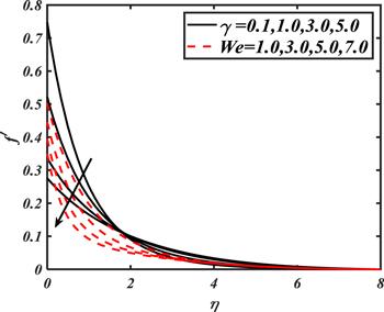
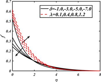
The graphical explanations are disclosed in figure 2 for the variation of $\gamma $ and We on ${f}^{{\prime} }$. The observations captured for the variation of $\gamma $ witness that velocity distribution declines with increasing $We.$ In fact, the involvement of viscosity related to the dimensionless Weissenberg number resists the velocity of accelerated fluid particles. The results for $\gamma $ show that the velocity profile altered due to the presence of slip factor. A decreasing behavior for $f^{\prime} $ is observed as $\gamma $ attained increasing values. The graphical observation based on a variation of $\lambda $ and $\delta $ is disclosed in figure 3. An increment in $\lambda $ shows stronger velocity distribution. Further, with the increase of $\delta ,$ velocity distribution boosts up initially with a minor variation and later on decreases as $\delta $ gets maximum values.
Figure 2.
 New window|Download| PPT slide
Figure 2.Impacts of $\gamma $ and $We$ on $f^{\prime} .$
Figure 3.
 New window|Download| PPT slide
Figure 3.Impacts of $\delta $ and $\lambda $ on $f^{\prime} .$
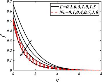
Figure 4 shows the importance of ${\rm{\Gamma }}$ and $Nc$ on $f^{\prime} .$ The velocity distribution decays by varying both flow parameters. The increment in $Nc$ is physical enrolled with the buoyancy forces, which decrease the movement of fluid particles. However, the decreasing trend due to Nc is more dominant than compared to ${\Gamma }$.
Figure 4.
 New window|Download| PPT slide
Figure 4.Impacts of ${\rm{\Gamma }}$ and $Nc$ on $f^{\prime} .$
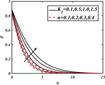
Figure 5 is prepared in order to detect the impact of ${K}_{1}$ and $n$ on $\theta .$ It is observed that with a variation of ${K}_{1},$ the temperature distribution is enhanced. Similarly, the increasing variation of $n$ also increases the temperature distribution due to shear thinning features.
Figure 5.
 New window|Download| PPT slide
Figure 5.Impacts of ${K}_{1}$ and $n$ on $\theta .$
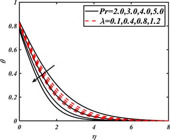
Figure 6 inspects the impact of $Pr$ and $\lambda $ on $\theta .$ The Prandtl number justifies the momentum and thermal diffusivity ratio. Due to the reverse relation with thermal diffusivity, the temperature distribution declines. With variation of $\lambda ,$ the heat transportation between the surfaces to fluid particles becomes slower.
Figure 6.
 New window|Download| PPT slide
Figure 6.Impacts of $Pr$ and $\lambda $ on $\theta .$
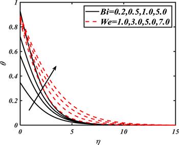
Figure 7 is plotted in order to visualize the characteristics of $Bi$ and $We$ on $\theta .$ It is noted that increasing values of $Bi$ maximize the variation in $\theta $ effectively. The enhancement in nanoparticles' temperature due to $Bi$ is physically validated as $Bi$ is directly related to $h.$ While observing the variation of $We$ on $\theta ,$ we noted that the nanoparticles' temperature also increases due to existence of viscosity.
Figure 7.
 New window|Download| PPT slide
Figure 7.Impacts of $Bi$ and $We$ on $\theta .$
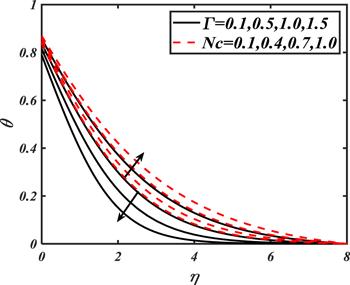
The impact of ${\rm{\Gamma }}$ and $Nc$ on $\theta $ are determined in figure 8. Various values have been chosen to investigate the variation of ${\rm{\Gamma }}$ on $\theta .$ The plot shows that $\theta $ increases with arising variation of ${\rm{\Gamma }}.$ For varying numerical values of $Nc,$ an increase in buoyancy ration forces causes an uplift in the nanoparticles' distribution.
Figure 8.
 New window|Download| PPT slide
Figure 8.Impacts of ${\rm{\Gamma }}$ and $Nc$ on $\theta .$
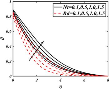
From figure 9, it is seen that the nanoparticles' temperature enhanced for varying $Nt$ and $Rd.$ The thermophoresis phenomenon occurs due to a temperature gradient between nanoparticles in which tinny fluid particles move from the surface of the cold to hot region. Due to this migration process, the thermal boundary layer increases. The physical consequences for utilization of $Rd$ on $\theta $ show that the nanoparticles' temperature is improved as the radiation source is being considered a more efficient heat transfer mode.
Figure 9.
 New window|Download| PPT slide
Figure 9.Impacts of $Nt$ and $Rd$ on $\theta .$
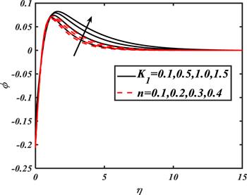
The variation in concentration distribution for various values of ${K}_{1}$ and $n$ is revealed in figure 10. The nanoparticles' concentration increases for leading values of both ${K}_{1}$ and $n.$
Figure 10.
 New window|Download| PPT slide
Figure 10.Impacts of ${K}_{1}$ and $n$ on $\phi .$
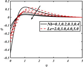
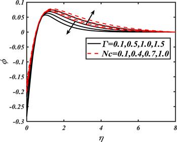
In order to look at the consequences of $Nb$ and $Le$ on $\phi ,$ figure 11 is sketched. Both parameters play a valuable role to control the nanoparticles' concentration in the whole distribution. Since Brownian motion signifies the random movement of nanoparticles over a moving configuration, which reduces as $Nb$ assigned maximum numerical values. On the other hand, Le is inversely related to the mass diffusivity. Therefore, the larger values of $Le$ decreases the mass diffusivity of the nanoparticles, which results in a decay in the nanoparticles' concentration profile. From figure 12, it is examined that the nanoparticles' distribution is resulted with a variation of $Nc$ while a reverse trend is noted for ${\rm{\Gamma }}.$
Figure 11.
 New window|Download| PPT slide
Figure 11.Impacts of $Nb$ and $Le$ on $\phi .$
Figure 12.
 New window|Download| PPT slide
Figure 12.Impacts of ${\rm{\Gamma }}$ and $Nc$ on $\phi .$
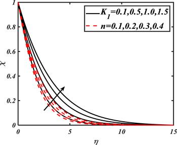
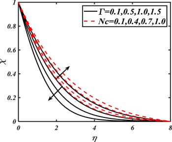
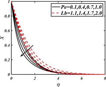
The impacts of various parameters such as ${K}_{1},$ $n,$ ${\rm{\Gamma }},$ $Nc,$ $Pe$ and $Lb$ on motile microorganisms distribution $\chi $ are disclosed in figures 13-15. Figure 13 exhibits the influence of ${K}_{1}$ and $n$ on $\chi .$ The motile microorganisms distribution increases with ${K}_{1}.$ The larger values of $n$ correspond to the shear thinning case which improve the motile microorganisms profile. From figure 14, it has been examined that the unsteady parameter controls the microorganisms' profile while $Nc$ results in an improved microorganisms' profile due to the existence of buoyancy forces. The variation in $\chi $ for different values of $Pe$ and $Lb$ is reported in figure 15. With an increase of $Pe$ motile diffusivity decreases, which increases the motile microorganism profile. Similarly, with the increment in $Lb$ also decay the motile microorganisms profile effectively.
Figure 13.
 New window|Download| PPT slide
Figure 13.Impacts of ${K}_{1}$ and $n$ on $\chi .$
Figure 14.
 New window|Download| PPT slide
Figure 14.Impacts of ${\rm{\Gamma }}$ and $Nc$ on $\chi .$
Figure 15.
 New window|Download| PPT slide
Figure 15.Impacts of $Pe$ and $Lb$ on $\chi .$
Table 1 represents the variation of $-f^{\prime\prime} (0)$ for some numerical values of $Ha,$ ${\rm{\Gamma }},$ $Nr,$ $Nc,$ $n,$ $We$ and $\gamma .$ An increasing value of $-{f}^{{\prime} ^{\prime} }(0)$ has been examined for $Ha,$ $Nc,$ $n$ and $We.$ The variation in $-{f}^{{\prime} ^{\prime} }(0)$ is quite minimal by increasing the slip factor $\gamma .$ In order to evaluate the significance of local Nusselt number $-\theta ^{\prime} (0)$ for iterating values of $Ha,$ ${\rm{\Gamma }},$ $Nr,$ $Nc,$ $n,$ $We,$ $Pr,$ $Nt,$ $Nb$ and $\gamma ,$ table 2 is prepared. The heat transfer rate is increased with $Pr,$ ${\rm{\Gamma }}$ while an opposite trend has been captured for all remaining parameters. From table 3, it is noted that the local Sherwood number attained maximum values for ${\rm{\Gamma }},$ $Nc$ and $Le.$ Finally, the numerical computation for the motile density number is inspected in table 4. A maximum variation in motile density number is observed for ${\rm{\Gamma }},$ $Nr$ and $Pe.$
Table 1.
Table 1.Variations of $-f^{\prime\prime} (0)$ for various values of involved parameters.
| $Ha$ | ${\rm{\Gamma }}$ | $Nr$ | $Nc$ | $n$ | $We$ | $\gamma $ | $-f^{\prime\prime} (0)$ |
|---|---|---|---|---|---|---|---|
| 0.1 | 0.2 | 0.5 | 0.5 | 0.3 | 0.3 | 1 | 0.3937 |
| 0.6 | 0.4740 | ||||||
| 1.2 | 0.5411 | ||||||
| 0.5 | 0.1 | 0.5219 | |||||
| 0.3 | 0.4790 | ||||||
| 0.5 | 0.4423 | ||||||
| 0.2 | 0.1 | 0.4618 | |||||
| 0.4 | 0.4605 | ||||||
| 0.7 | 0.4592 | ||||||
| 0.5 | 0.1 | 0.4249 | |||||
| 0.4 | 0.4523 | ||||||
| 0.7 | 0.4816 | ||||||
| 0.5 | 0.1 | 0.4383 | |||||
| 0.4 | 0.4751 | ||||||
| 0.7 | 0.5288 | ||||||
| 0.3 | 0.1 | 0.4577 | |||||
| 0.5 | 0.4659 | ||||||
| 1.0 | 0.4763 | ||||||
| 0.1 | 2.0 | 0.2859 | |||||
| 3.0 | 0.2078 | ||||||
| 4.0 | 0.1634 |
New window|CSV
Table 2.
Table 2.Variations of $-\theta ^{\prime} (0)$ for various values of involved parameters.
| $Ha$ | ${\rm{\Gamma }}$ | $Nr$ | $Nc$ | $n$ | $We$ | $Pr$ | $Nt$ | $Nb$ | $-\theta ^{\prime} (0)$ |
|---|---|---|---|---|---|---|---|---|---|
| 0.1 | 0.2 | 0.5 | 0.5 | 0.3 | 0.3 | 2.0 | 0.3 | 0.2 | 0.2368 |
| 0.6 | 0.2055 | ||||||||
| 1.2 | 0.1775 | ||||||||
| 0.5 | 0.1 | 0.1689 | |||||||
| 0.3 | 0.2003 | ||||||||
| 0.5 | 0.2203 | ||||||||
| 0.2 | 0.1 | 0.2112 | |||||||
| 0.4 | 0.2111 | ||||||||
| 0.7 | 0.3210 | ||||||||
| 0.5 | 0.1 | 0.2216 | |||||||
| 0.4 | 0.2140 | ||||||||
| 0.7 | 0.2064 | ||||||||
| 0.5 | 0.1 | 0.2181 | |||||||
| 0.4 | 0.2078 | ||||||||
| 0.7 | 0.1972 | ||||||||
| 0.3 | 0.1 | 0.2127 | |||||||
| 0.5 | 0.2098 | ||||||||
| 1.0 | 0.2063 | ||||||||
| 0.1 | 1.0 | 0.1589 | |||||||
| 3.0 | 0.2486 | ||||||||
| 5.0 | 0.3000 | ||||||||
| 2.0 | 0.1 | 0.2183 | |||||||
| 0.5 | 0.2044 | ||||||||
| 0.8 | 0.1948 |
New window|CSV
Table 3.
Table 3.Variations of $-\phi ^{\prime} (0)$ for various values of involved parameters.
| $Ha$ | ${\rm{\Gamma }}$ | $Nr$ | $Nc$ | $n$ | $We$ | $Pr$ | $Le$ | $-\phi ^{\prime} (0)$ |
|---|---|---|---|---|---|---|---|---|
| 0.1 | 0.2 | 0.5 | 0.5 | 0.3 | 0.3 | 2.0 | 0.3 | 0.3551 |
| 0.6 | 0.3082 | |||||||
| 1.2 | 0.2662 | |||||||
| 0.5 | 0.1 | 0.2548 | ||||||
| 0.3 | 0.3005 | |||||||
| 0.5 | 0.3304 | |||||||
| 0.2 | 0.1 | 0.3169 | ||||||
| 0.4 | 0.3167 | |||||||
| 0.7 | 0.3165 | |||||||
| 0.5 | 0.1 | 0.3325 | ||||||
| 0.4 | 0.3210 | |||||||
| 0.7 | 0.3079 | |||||||
| 0.5 | 0.1 | 0.3272 | ||||||
| 0.4 | 0.3117 | |||||||
| 0.7 | 0.2960 | |||||||
| 0.3 | 0.1 | 0.3190 | ||||||
| 0.5 | 0.3147 | |||||||
| 1.0 | 0.3094 | |||||||
| 0.1 | 1.0 | 0.2383 | ||||||
| 3.0 | 0.3729 | |||||||
| 5.0 | 0.4500 | |||||||
| 2.0 | 1.0 | 0.3206 | ||||||
| 2.0 | 0.3172 | |||||||
| 3.0 | 0.3163 |
New window|CSV
Table 4.
Table 4.Variations of $-\chi ^{\prime} (0)$ for various values of involved parameters.
| $Ha$ | ${\rm{\Gamma }}$ | $Nr$ | $Nc$ | $n$ | $We$ | $Pe$ | $Lb$ | $-\chi ^{\prime} (0)$ |
|---|---|---|---|---|---|---|---|---|
| 0.1 | 0.2 | 0.5 | 0.5 | 0.3 | 0.3 | 0.2 | 2.0 | 0.7875 |
| 0.6 | 0.6917 | |||||||
| 1.2 | 0.6016 | |||||||
| 0.5 | 0.1 | 0.5969 | ||||||
| 0.3 | 0.6796 | |||||||
| 0.5 | 0.7349 | |||||||
| 0.2 | 0.1 | 0.7087 | ||||||
| 0.4 | 0.7096 | |||||||
| 0.7 | 0.7099 | |||||||
| 0.5 | 0.1 | 0.7467 | ||||||
| 0.4 | 0.7188 | |||||||
| 0.7 | 0.6969 | |||||||
| 0.5 | 0.1 | 0.7326 | ||||||
| 0.4 | 0.6959 | |||||||
| 0.7 | 0.6516 | |||||||
| 0.3 | 0.1 | 0.7133 | ||||||
| 0.5 | 0.7040 | |||||||
| 1.0 | 0.6925 | |||||||
| 0.1 | 0.2 | 0.7383 | ||||||
| 0.6 | 0.8596 | |||||||
| 1.0 | 0.9816 | |||||||
| 0.2 | 0.1 | 0.4603 | ||||||
| 0.5 | 0.5950 | |||||||
| 1.0 | 0.6661 |
New window|CSV
5. Conclusions
In this investigation, the slip flow of a non-Newtonian nanoliquid has been considered in the presence of activation energy and nonlinear thermal radiation. The flow problem is modeled, which is numerically treated by employing the shooting algorithm. The achieved results are summarized as follows: The distribution of velocity is altered slowly with interaction of slip factors, unsteady parameter and Rayleigh number.The temperature distribution is enhanced in case of shear thinning and thermal Biot number.
The Brownian motion parameter and Lewis number reduce the nanoparticles' concentration distribution.
The local Nusselt number, local Sherwood number and motile density number increase with higher unsteady parameters.
The reported continuations may involve applications of thermal extrusion systems and solar energy processes.
Current analysis has been further extended for three-dimensional flow and by performing stability analysis.
Acknowledgments
The authors extended their appreciation to the Deanship of Scientific Research at King Khalid University for funding this work through Research Groups Program under grant number (R.G.P.2/66/40).Reference By original order
By published year
By cited within times
By Impact factor
[Cited within: 1]
DOI:10.1016/j.ijheatmasstransfer.2017.01.044 [Cited within: 1]
DOI:10.1016/j.ijheatmasstransfer.2017.03.037 [Cited within: 1]
DOI:10.1371/journal.pone.0168824 [Cited within: 1]
DOI:10.1108/MMMS-08-2018-0146 [Cited within: 1]
DOI:10.3390/mi10060373 [Cited within: 1]
DOI:10.1016/j.ijheatmasstransfer.2017.05.042 [Cited within: 1]
DOI:10.1016/j.molliq.2019.04.130 [Cited within: 1]
DOI:10.1016/j.powtec.2018.09.093 [Cited within: 1]
DOI:10.1016/j.jestch.2018.02.007 [Cited within: 1]
DOI:10.1016/j.rinp.2017.12.013 [Cited within: 1]
DOI:10.1007/s10973-019-08555-4 [Cited within: 1]
DOI:10.1088/1402-4896/ab0661 [Cited within: 1]
DOI:10.1007/s10483-019-2518-9 [Cited within: 1]
DOI:10.1016/j.cma.2018.04.020 [Cited within: 1]
DOI:10.1007/s10483-020-2581-5 [Cited within: 1]
DOI:10.1016/j.chaos.2020.109656 [Cited within: 1]
DOI:10.1016/j.molliq.2019.111939 [Cited within: 1]
DOI:10.1016/j.icheatmasstransfer.2010.08.015 [Cited within: 1]
DOI:10.1016/j.apt.2016.10.002 [Cited within: 1]
DOI:10.3390/pr7110859 [Cited within: 1]
DOI:10.1016/j.cjph.2017.08.031 [Cited within: 1]
DOI:10.1016/j.physb.2017.09.128 [Cited within: 1]
DOI:10.1016/j.ijheatmasstransfer.2017.05.005 [Cited within: 1]
DOI:10.1016/j.euromechflu.2019.01.002 [Cited within: 1]
DOI:10.1002/htj.21403 [Cited within: 1]
DOI:10.1088/1402-4896/ab194a [Cited within: 1]
DOI:10.1016/j.rinp.2016.09.006 [Cited within: 1]
DOI:10.1016/j.icheatmasstransfer.2017.11.001
DOI:10.1002/htj.21451
DOI:10.1016/j.energy.2019.116801 [Cited within: 1]
DOI:10.1016/0095-8522(65)90022-X [Cited within: 2]
DOI:10.1016/j.ijheatmasstransfer.2018.11.022 [Cited within: 2]
DOI:10.1063/1.3052923 [Cited within: 1]
DOI:10.3390/sym12020309
DOI:10.1515/jnet-2019-0049
DOI:10.1088/1402-4896/ab399f [Cited within: 1]
