O. Langueur¹, M. Merad^,1,*, B. Hamil²1 Département des sciences de la matière, Faculté des Sciences Exactes, Université de Oum El Bouaghi, 04000 Oum El Bouaghi, Algeria
2 Département de TC de SNV, Université Hassiba Benbouali, Chlef, Algeria;3 School of Information and Control Engineering, Xi'an University of Architecture and Technology, Xi'an 710055, China

Corresponding authors: *E-mail:meradm@gmail.com

Received:2019-03-17Accepted:2019-04-22Online:2019-09-1


Abstract
In this work, we study the DKP equation subjected to the action of combined vector plus scalar energy depend on potentials in (1+1) dimensions space-time. The conditions of normalisation and continuity equation are calculated. The eigenfunctions and the corresponding eigenvalues are then determined. A numerical study is presented and the energy graphs for some values of the energy parameter are plotted.
Keywords： DKP equation;energy dependent potentials;biconfluent Heun function


PDF (134KB)MetadataMetricsRelated articlesExportEndNote|Ris|BibtexFavorite
Cite this article
O. Langueur, M. Merad, B. Hamil. DKP Equation with Energy Dependent Potentials. [J], 2019, 71(9): 1069-1074 doi:10.1088/0253-6102/71/9/1069

1 Introduction

For a long time, works on the so called systems with energy dependent potentials^[1] have raised a considerable interest because of its varied applications in several areas and their analyses does not cease developing. We quote some examples, the dynamo effect in magneto hydrodynamic models,^[2] in quantum wells and semiconductors,^[3] including the theory of elastic and inelastic scattering in atomic, nuclear and particle physics,^[4-5] and the description of the heavy quark system^[6-7] etc. Further, we point out that systems with energy-dependent potentials provide some modifications on the mathematical structure as the scalar product and the completeness relation, necessary to ensure conservation of the norm and satisfy the requirements of quantum mechanics, which has been analyzed clearly in Refs. [6] and [8].

For this purpose, the treatment of the potential-dependent energy, continues to increase, consequently numerous works were looked and several methods of analytical and approximate resolution were presented. Let us mention one of these potentials: the harmonic oscillator with an energy-dependent frequency in 1D and in 3D which has recently been solved,^{[6, 9]} the Coulomb and the Morse potentials,^[10-11] the harmonic oscillator and the P?schl-Teller potential by means of the supersymmetry formalism.^[12] The D-dimensional Schr?dinger and Klein-Gordon equations were studied via the Nikiforov-Uvarov method,^[13-14] a class of potentials was perfectly resolvable by the conversion method,^[11] the approximate solution of the Dirac equation using the supersymmetry quantum mechanics.^[15] Dirac particles in the presence of scalar, vector, and tensor potentials have been investigated by using the asymptotic iteration method,^[16] extension to the case of systems having mass dependent position were examined in Ref. [17]. The harmonic oscillator and the hydrogen atom and the Klein-Gordon particle subjected to vector plus scalar energy dependent potentials were examined by using the Feynman approach.^[18-19] The Dirac propagator was determined by using the formalism for supersymmetric path integrals^[20] and the harmonic oscillator propagator has been constructed via the path integral approach in noncommutative space.^[21-22]

In the present paper we extend this idea to the another relativistic equation namely Duffin-Kemmer-Petiau (DKP) equation, other than that of Dirac and Klein-Gordon, describing the dynamics of the scalar and vectorial Bosons. The DKP equation is of great importance of these various applications in quantum chromodynamics, cosmology, gravity, and its richness of these experimentation in areas of physics.^[23] To our knowledge, this equation has never been treated with energy-dependent potential, in an analytical manner and its absence is practically noticeable in the context of problems with energy dependent potentials.

In this paper, we will try to study the DKP equation subjected to the action of combined with vector and scalar energy-dependent potentials in (1+1) dimensions space-time on the one hand, and on the other hand to see the effect of this energy dependence on the normalisation conditions and the continuity equation for this system in question.

The outline of this paper is as follows: In Sec. 2, we determine the normalisation condition and continuity equation for (DKP) equation. In Sec. 3, we expose an explicit calculation relative to the one-dimensional (DKP) subjected to the action of combined with vector and scalar energy-dependent potentials. By a straightforward calculation, the exact solution is obtained and the energy spectrum and wave functions are deduced. These latter are expressed by the biconfluent Heun polynomials. In Sec. 4, a numerical study of the energy function is presented.

2 Normalization Condition and Continuity Equation

The (1+1)-dimensional DKP equation for the scalar and vector bosons moving in a constant electric field and a scalar potential is:

(1)$[ \beta^{0} ( i\partial_{0}-eV( x,i\partial_{0}) ) +i\beta^{1}\partial_{x}-( m+S( x,i\partial_{0}) ) ] \psi=0\,,$
where the matrices $\beta^{0}$ and $\beta^{1}$ verify the DKP algebra

(2)$\beta^{\mu}\beta^{\nu}\beta^{\alpha}+\beta^{\alpha}\beta^{\nu}\beta^{\mu }=g^{\mu\nu}\beta^{\alpha}+g^{\alpha\nu}\beta^{\mu}\,, $
and the potentials $V\left( x,i\partial_{0}\right) $ $ $and $ S\left(x,i\partial_{0}\right) $ denote a function of $x$ and energy $i\partial_{0}$.

The metric tensor $g^{\mu\nu}={\rm diag}(\begin{array}[c]{cc}1 & -1\end{array}) ,$ and the adjoint spinor $\bar{\psi}=\psi^{+}\left( 2\beta_{0}^{2}-1\right) $ verifies the following adjoint equation

(3)$\big\{ \big[ \left( -i\partial_{0}-eV\left( x,i\partial_{0}\right) ^{\ast}\right) \bar{\psi}\beta^{0}\big] -i\left( \partial_{x}\bar{\psi }\right) \beta^{1}\nonumber\\ \quad -\left[ m+S\left( x,i\partial_{0}\right) ^{\ast }\right] \bar{\psi}\big\} =0\,. $
If we expand $\psi$ on the basis $\left\{ \Phi_{E_{n}}\right\} $

(4)$\psi=\sum_{n}a_{E_{n}}\Phi_{E_{n}}e^{-i E_{n}t}, $
we have

(5)$\left[ \beta^{0}\left( E_{n}-eV\left( x,E_{n}\right) \right) +i\beta ^{1}\partial_{x}-\left( m+S\left( x,E_{n}\right) \right) \right] \Phi_{E_{n}} =0\,, $
(6)$\left\{ \left[ \left( E_{m}-eV\left( x,E_{m}\right) \right) \bar{\Phi }_{E_{m}}\beta^{0}\right] -i\left( \partial_{x}\bar{\Phi}_{E_{m}}\right) \beta^{1}-\left( m+S\left( x,E_{m}\right) \right) \bar{\Phi}_{E_{m} }\right\} =0\,. $
By multiplying Eq. (5) by $\bar{\Phi}_{E_{m}}$ and the adjoint equation (6) by $\Phi_{E_{n}},$ and after subtraction and integration over d$x$, we obtain the orthogonality relation between two states $n$ and $m$

(7)$int d x\bar{\Phi}_{E_{m}}\left\{ \beta^{0}-\beta^{0}e\frac{V\left( x,E_{n}\right) -V\left( x,E_{m}\right) }{E_{n}-E_{m}}-\frac{S\left( x,E_{n}\right) -S\left( x,E_{m}\right) }{E_{n}-E_{m}}\right\} \Phi_{E_{n} }=\delta_{nm}\,,$
and, in the limit $n\rightarrow m,$ the above equation becomes

(8)$int d x\bar{\Phi}_{E}\left\{ \beta^{0}-\phi_{nn}\right\} _{E=E_{n}}\Phi _{E}=1\,,$
where

(9)$\phi_{nn}=\beta^{0}e\frac{\partial V\left( x,E\right) }{\partial E} -\frac{\partial S\left( x,E\right) }{\partial E}\,. $
Therefore, the presence of the additional factor $\left\{ \beta^{0}-\phi _{nn}\right\} $ changes the scalar product (the norm). In the case where the potential does not depend on energy $\phi_{nn}=0,$ we find the usual normalization condition $int d x\bar{\Phi}_{E}\beta^{0}\Phi_{E}=1$.

Now, to derive the continuity equation $\partial_{\mu}J^{\mu}=\partial _{\mu}\bar{\psi}\beta^{\mu}\psi=0$, multiplying Eq. (1) by $\left( \bar{\psi}\right) $ and Eq. (3) by $\left( \psi\right) $ and differentiating between the two equations, we obtain the following expression

(10)$\partial_{x} J^{1} =\partial_{x}\bar{\psi}\beta^{1}\psi\,,$
(11)$\partial_{0}\rho =\partial_{0}\bar{\psi}\beta^{0}\psi-\frac{e}{i}\left\{ \bar{\psi}\beta^{0}V\left( x,i\partial_{0}\right) \psi-\left[ V\left( x,i\partial_{0}\right) ^{\ast}\bar{\psi}\right] \beta^{0}\psi\right\}\\ \quad \qquad-\frac{1}{i}\left\{ \bar{\psi}S\left( x,i\partial_{0}\right) \psi-\left[ S\left( x,i\partial_{0}\right) ^{\ast}\bar{\psi}\right] \psi\right\} . $
To simplify the form of $\rho$, we put this separate formed,

(12)$V\left( x,i\partial_{0}\right) =U\left( x\right) +V\left( x\right) i\partial_{0}\,,$
(13)$S\left( x,i\partial_{0}\right) =S_{0}\left( x\right) +S_{1}\left( x\right) i\partial_{0}\,,$
(14)$\psi =\sum_{n}a_{E_{n}}e^{-i E_{n}t}\Phi_{E_{n}}\,.$
After a direct calculation, the expression of the density $\rho$ can be rewritten as

(15)$\rho=\sum_{n,m}a_{E_{n}}a_{E_{m}}^{\ast}\bar{\Phi}_{E_{m}}\beta^{0} \Phi_{E_{n}}e^{i\left( E_{m}-E_{n}\right) t}-eV\left( x\right) \sum _{n,m}a_{E_{n}}a_{E_{m}}^{\ast}\frac{\left\{ E_{m}\bar{\Phi}_{E_{m}}\beta ^{0}\Phi_{E_{n}}-\bar{\Phi}_{E_{m}}\beta^{0}\Phi_{E_{n}}E_{n}\right\} }{\left( E_{m}-E_{n}\right) }e^{i\left( E_{m}-E_{n}\right) t} \\ \quad -\frac{eV\left( x\right) }{i}C^{st}\sum_{n,m}a_{E_{n}}a_{E_{m}}^{\ast }\left\{ E_{m}\bar{\Phi}_{E_{m}}\beta^{0}\Phi_{E_{n}}-\bar{\Phi}_{E_{m}} \beta^{0}\Phi_{E_{n}}E_{n}\right\} \\ \quad -S_{1}\left( x\right) \sum_{n,m}a_{E_{n}}a_{E_{m}}^{\ast}e^{i\left( E_{m}-E_{n}\right) t}\bar{\Phi}_{E_{m}}\Phi_{E_{n}}-\frac{1}{i}S_{1}\left( x\right) C^{st}\sum_{n,m}a_{E_{n}}a_{E_{m}}^{\ast}\left\{ E_{n} -E_{m}\right\} \bar{\Phi}_{E_{m}}\Phi_{E_{n}}\,,$
and by taking the lim $n\rightarrow m$, Eq. (15) will be reduced to this form

(16)$\rho=\bar{\psi}\beta^{0}\psi\left( 1-eV\left( x\right) \right) -S_{1}\left( x\right) \bar{\psi}\psi\,.$

3 DKP Equation in a Constant Electric Field and a Scalar Potential

In this section we illustrate the energy dependent potentials on the energy eigenvalues and eigenfunctions of a DKP particle in a constant electric field and a scalar potential. The electric field and the scalar potential are chosen linear

(17)$V\left( x\right) =V_{0}A_{E}x\,, \quad S\left( X\right) =S_{0}A_{E}x\,, $
where $V_{0}$ and $S_{0}$ two constants, we suppose $\left\vert S_{0} \right\vert \succ\left\vert V_{0}\right\vert $ to avoid complex eigenvalues, and $A_{E}=\left( 1+\theta E\right) ^{q}$.

In (1+1)-dimensional space time, we choose this representation of the following

DKP matrix $\beta$,

(18)$\beta^{0}=\left( \begin{array} [c]{ccc} 0 & 0 & i\\ 0 & 0 & 0\\ -i & 0 & 0 \end{array} \right) ,\quad \beta^{1}=\left( \begin{array} [c]{ccc} 0 & i & 0\\ i & 0 & 0\\ 0 & 0 & 0 \end{array} \right) . $
Hence, the DKP equation in the presence of a vector plus scalar with energy dependent potentials is written as

(19)$\Bigl[ \beta^{0}\Bigl( \frac{i\partial}{\partial t}-V\Bigl( x,\frac {i\partial}{\partial t}\Bigr) \Bigr) +i\beta^{1}\frac{\partial}{\partial x}-\Bigl( m+S\Bigl( x,\frac{i\partial}{\partial t}\Bigr) \Bigr) \Bigr]\\ \;\;\times\psi=0\,.$
The stationary solution of Eq. (19) has the form $\psi\left( x,t\right) =\phi\left( x\right) e^{-i Et}$ and $\phi\left( x\right) $ is a vectors of dimension $(3 \times 1)$ which can be written as

(20)$\phi^{{\rm T}}=( \begin{array} [c]{ccc} \phi_{1} & \phi_{2} & \phi_{3} \end{array} )\,. $
We insert the wave function $\phi$ and the matrix $\beta$, we obtain the following equations systems

(21)$\quad i\left(E-V\left( x,E\right) \right) \phi_{3}-\frac{d}{d x}\phi_{2}-\left( m+S\left( x,E\right) \right) \phi_{1}=0\,,\\ \quad\frac{d}{d x}\phi_{1}+\left( m+S\left( x,E\right) \right) \phi_{2}=0\,,\\ \quad i\left( E-V\left( x,E\right) \right) \phi_{1}+\left( m+S\left( x,E\right) \right) \phi_{3}=0\,. $
Now, to solve the eigenvalue equation (19), we decouple the system (21) and it is not difficult to verify that $\phi_{1}$ satisfies the following Klein Gordon type equation

(22)$\Bigl[ \frac{d^{2}}{d x^{2}}-\frac{1}{\left( {m}/{S_{0}A_{E}}+x\right) }\frac{d}{d x}-\mu\Bigl( x+\frac{\eta}{\mu}\Bigr) ^{2}+\frac{\eta^{2}}{\mu }-\vartheta^{2}\Bigr]\\ \quad \;\;\times\phi_{1}=0\,, $
where

(23)$\mu=\left( S_{0}^{2}-V_{0}^{2}\right) A_{E}^{2}\,, \quad\eta=A_{E}\left( mS_{0}+EV_{0}\right)\,,\\{\rm and}\quad \vartheta^{2}=m^{2}-E^{2}\,, $
and we introduce the following ansatz

(24)$\phi_{1}(x)=e^{int^{x}f\left( u\right) d u}\Phi\left( x\right), $
where $f\left( x\right) $ is arbitrary function. Then, the equation for

$\Phi\left( x\right) $ is

(25)$\Bigl[ \frac{d^{2}}{d x^{2}}+\Bigl( 2f-\frac{1}{\left({m}/{S_{0}A_{E} }+x\right) }\Bigr) \frac{d}{d x}-\frac{f}{\left({m}/{S_{0}A_{E} }+x\right) }\\ \quad +f^{\prime}+f^{2}-\mu\Bigl( x+\frac{\eta}{\mu}\Bigr) ^{2}+\frac{\eta^{2}}{\mu}-\vartheta^{2}\Bigr] \Phi=0\,. $
We choose $f\left(x\right)$ to cancel the term $\left(x+({\eta}/{\mu})\right) $, this implies

(26)$f\left( x\right) =-\mu^{{1}/{2}}\Bigl(x+\frac{\eta}{\mu}\Bigr)\,. $
By substituting $f\left(x\right)$ with their expression (26) and changing the variable from $x$ to $y$, by setting $y=\mu^{{1}/{4}}( x+({m}/{S_{0}A_{E}}))$, then Eq. (25) can be expressed as

(27)$\qquad \Bigl\{ \frac{d^{2}}{d y^{2}}+\Bigl[\frac{\alpha+1}{y}-2y-\beta\Bigr] \frac{d}{d y}\\ \qquad \quad +\,\Bigl[ ( \gamma-\alpha-2) -\frac{\delta +\beta\left( \alpha+1\right) }{2y}\Bigr] \Bigr\} \Phi =0\,,$
which is exactly the biconfluent Heun differential equation HeunB$\left(\alpha,\beta,\gamma,\delta,y\right)$,^[23-24] whose parameters $\alpha,$ $\beta,$ $\gamma$, and $\delta$ are given by

(28)$\alpha=-2\,,\quad \beta=2\mu^{{1}/{4}}\left( \frac{\eta}{\mu} -\frac{m_{0}}{S_{0}A_{E}}\right)\,,\\ \gamma=\mu^{-{1}/{2}}\left( \frac{\eta^{2}}{\mu}-\vartheta^{2}\right)\,, \quad\delta=0\,. $
The above differential equation (27) has one regular singularity at theorigin $(y=0)$, and one irregular singularity at infinity $(y\rightarrow\infty)$ whose s-rank is $R(\infty)=3$, its solution can be expressed as Eq. (52) (see Appendix):

(29)$\Phi=C_{1}{\rm HeunB}\left( \alpha,\beta,\gamma,\delta,y\right) +C_{2}y^{-\alpha }{\rm HeunB}\\ \times\left( -\alpha,\beta,\gamma,\delta,y\right), $
where $C_{1}$, $C_{2}$ are constant.

The determination of the other components is easy and the final expressions of wave function are as follows:

(30)$\phi_{1}(x) =e^{-({\sqrt{\mu}}/{2})\left( x+({eta}/{\mu})\right) ^{2}}\Bigl\{ C_{1}{\rm HeunB}\Bigl( -2,\beta,\gamma,0,\mu^{{1}/{4}}\Bigl( x+\frac{m}{S_{0}A_{E}}\Bigr) \Bigr) \\ \quad\quad\quad\ +C_{2}\sqrt{\mu}\Bigl( x+\frac{m}{S_{0}A_{E}}\Bigr) ^{2}{\rm HeunB}\Bigl( 2,\beta,\gamma,0,\mu^{{1}/{4}}\Bigl( x+\frac{m} {S_{0}A_{E}}\Bigr) \Bigr) \Bigr\}, $
(31)$\phi_{2}(x) =-\frac{1}{m+S\left( x,E\right) }\frac{d}{d x}\Bigl\{ e^{-({\sqrt{\mu}}/{2})\left(x+{eta}/{\mu}\right) ^{2}}\Bigl[ C_{1}{\rm HeunB}\Bigl( -2,\beta,\gamma,0,\mu^{{1}/{4}}\Bigl(x+\frac{m} {S_{0}A_{E}}\Bigr) \Bigr) \\ \quad\quad\quad\ +C_{2}\sqrt{\mu}\Bigl( x+\frac{m}{S_{0}A_{E}}\Bigr) ^{2}{\rm HeunB}\Bigl( 2,\beta,\gamma,0,\mu^{{1}/{4}}\Bigl( x+\frac{m} {S_{0}A_{E}}\Bigr) \Bigr) \Bigr] \Bigr\} , $
(32)$\phi_{3}(x) =-i\frac{\left( E-e_{0}V\left( x,E\right) \right) }{m+S\left( x,E\right) }e^{-({\sqrt{\mu}}/{2})\left(x+({eta}/{\mu })\right) ^{2}}\Bigl\{ C_{1}{\rm HeunB}\Bigl( -2,\beta,\gamma,0,\mu^{{1}/{4} }\Bigl( x+\frac{m}{S_{0}A_{E}}\Bigr) \Bigr) \\ \quad\quad\quad\ +C_{2}\sqrt{\mu}\Bigl( x+\frac{m}{S_{0}A_{E}}\Bigr) ^{2}{\rm HeunB}\Bigl( 2,\beta,\gamma,0,\mu^{{1}/{4}}\Bigl( x+\frac{m} {S_{0}A_{E}}\Bigr) \Bigr) \Bigr\}\,. $
Now, to determine energy spectrum, using the condition $\left( 53\right)$ $\left(\text{see appendix}\right)$ and replacing the parameters $\alpha$ and $\gamma$ by their expressions (28), we finally get the following result

(33)$E^{2}-m^{2}+\frac{\left( mS_{0}+EV_{0}\right) ^{2}}{\left( S_{0}^{2} -V_{0}^{2}\right) }-2n\sqrt{S_{0}^{2}-V_{0}^{2}}\left( 1+\theta E\right) ^{q}=0\,. $

4 Application

Now in our analysis, it is interesting to study two particular cases for values of $q$, we limit ourselves only to the case $q=1$ and $q=2$, for the other cases, the calculation becomes a little more complicated to determine exactly and analytically the values of the spectrum.

(i) First case: $q=1$: $A_{E}=\left( 1+\theta E\right) $, the potentials in Eq. (17) contain a linear energy-dependence, the expression of energy function can be written in the form

(34)$E^{2}-m^{2}+\frac{\left( mS_{0}+EV_{0}\right) ^{2}}{\left( S_{0}^{2} -V_{0}^{2}\right) }-2n\sqrt{S_{0}^{2}-V_{0}^{2}}\left( 1+\theta E\right) =0\,, $
which gives

(35)$E_{n}^{\pm}=\frac{1}{S_{0}^{2}}\big[ n\theta\left( S_{0}^{2}-V_{0} ^{2}\right) ^{{3}/{2}}-mS_{0}V_{0}\pm\sqrt{2nS_{0}\left( S_{0}-m\theta V_{0}\right) \left(S_{0}^{2}-V_{0}^{2}\right) ^{{3}/{2}}+n^{2} \theta^{2}\left( S_{0}^{2}-V_{0}^{2}\right) ^{3}}\,\big]\,, $
and expanding to the first order in $\theta$, we obtain

(36)$E_{n}^{\pm}=-\frac{m_{0}V_{0}}{S_{0}}\pm\frac{\sqrt{2n}\left( S_{0}^{2} -V_{0}^{2}\right)^{{3}/{4}}}{S_{0}}+\theta\Bigl[\frac{n\left( S_{0}^{2}-V_{0}^{2}\right) ^{{3}/{2}}}{S_{0}^{2}}\mp\frac{\sqrt {2n}mV_{0}\sqrt{2n}\left( S_{0}^{2}-V_{0}^{2}\right) ^{{3}/{4}}} {2S_{0}^{2}}\Bigr]. $
The first term in Eq. (36) is the energy spectrum of the usual DKP equation subjected to the action of combined vector plus scalar and the second term represents the effects of quantum fluctuations of the potential-dependent energy on the system. It is remarkable here that, the expression of the energy spectrum in our system (36) contains an additional deformed correction term depending on the deformation parameter $\theta$ and with powers in $n$ due to the dependence of energy potentials.

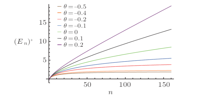
In Fig. 1, we notice that:

$\bullet$ The energy $E_{n}^{+}$ is presented as a function of $n$ for several values of $\theta$ and $n\leq160$. These energies take the positive values $\left( E_{n}^{+}\succeq0\right)$ for $n\succeq1$.

$\bullet$ For $ \theta$ negative, the spectrum is compressed and for $\theta$ positive, the spectrum is expanded, which produce an increase of the level spacing as a function of $n$, as the collective states of even-even atomic nuclei in the Bohr-Mottelson model, in particle physics phenomenology and in the physics beyond the standard model, etc.

$\bullet$ The function $E_{n}^{+}=f\left(n\right)$ is an increasing monotonous function for $\theta$ arbitrary and the beginning of the saturation depend of $\theta$ starts from a specific quantum number.

$\bullet$ It should be noted that, according to the powers in $n$ dependence of the energy levels, it explains confinement at the high energy area.

Fig. 1

New window|Download| PPT slide
Fig. 1(Color online) The plot illustrates the Spectrum of energy $\left( E_n\right) ^+$ verus quantum number $n$ with $V_0=0.3,S_0=0.5,m=1$.



(ii) Second case: $q=2$: $A_{E}=\left(1+\theta E\right)^{2}$, the potentials in Eq. (17) contain a quadratic energy-dependence, the formula of energy simplifies to

(37)$E^{2}-m^{2}+\frac{\left( mS_{0}+EV_{0}\right) ^{2}}{\left( S_{0}^{2} -V_{0}^{2}\right) }-2n\sqrt{S_{0}^{2}-V_{0}^{2}}( 1+\theta E) ^{2}=0\,, $
we get

(38)$E_{n}^{\pm}=\frac{2n\theta\left(S_{0}^{2}-V_{0}^{2}\right) ^{{3}/{2} }-mS_{0}V_{0}\pm\left( S_{0}-m\theta V_{0}\right) \sqrt{2n\left( S_{0} ^{2}-V_{0}^{2}\right) ^{{3}/{2}}}}{S_{0}^{2}-2n\theta^{2}\left( S_{0}^{2}-V_{0}^{2}\right) ^{{3}/{2}}}\,, $
and expanding to the second order in $\theta$, we obtain

(39)$E_{n}^{\pm} = frac{-mV_{0}}{S_{0}}\pm\frac{\left( S_{0}^{2}-V_{0} ^{2}\right) ^{{3}/{4}}\sqrt{2n}}{S_{0}}+\theta\Bigl[ \frac{2n\left( S_{0}^{2}-V_{0}^{2}\right) ^{{3}/{2}}}{S_{0}^{2}}\mp\frac{\sqrt {2n}mV_{0}\left( S_{0}^{2}-V_{0}^{2}\right)^{{3}/{4}}}{S_{0}^{2} }\Bigr]\\ -\theta^{2}\Bigl[\dfrac{2nmV_{0}\left(S_{0}^{2}-V_{0}^{2}\right) ^{{3}/{2}}}{S_{0}^{3}}\mp\dfrac{\left(2n\right) ^{{3}/{2}}\left( S_{0}^{2}-V_{0}^{2}\right) ^{{9}/{4}}}{S_{0}^{3}}\Bigr]\,, $
according to the factor $S_{0}^{2}-2n\theta^{2}\left(S_{0}^{2}-V_{0} ^{2}\right)^{{3}/{2}}$ (a denominator), which is presented in the energy formula (38), we clearly see the appearance of a critical point $\theta_{c}={S_{0}}/{\sqrt{2n(S_{0}^{2}-V_{0}^{2}) ^{{3}/{2}}}}.$

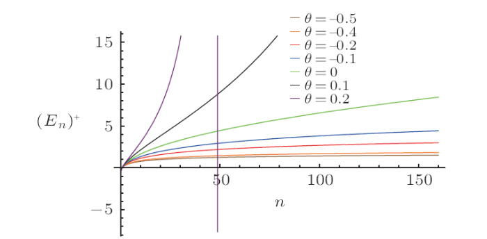
In Fig. 2, in this case, for $\theta\succ0$ there is an important observation, the energy as expanded and grows towards $\theta_{c}$, for example $30<n<50$, it corresponds $\theta_{c}=0.2$ and $ $for $ n\succ90$, it corresponds $\theta_{c}=0.1$, etc.

Fig. 2

New window|Download| PPT slide
Fig. 2(Color online) The plot illustrates the Spectrum of energy $\left(E_n\right)^+$ verus quantum number $n$ with $V_0=0.3$, $S_0=0.5$, $m=1$.



For $\theta\prec0$ the spectrum is compressed and there is saturation starts from a specific quantum number, depend of $\theta$. However, for a fixed value of $\theta$, the energy $E_{n}^{+}=f\left( n\right) $ is an increasing monotonous function.

In the end, for the two expressions of energy, in the $\lim\theta\rightarrow0$ returning to the ordinary case $A_{E}=1$, we get the usual expression of the energy spectrum of the ordinary DKP equation in the presence of electromagnetic field

(40)$E_{n}^{\pm}=-\frac{m_{0}V_{0}}{S_{0}}\pm\sqrt{2n\frac{\left( S_{0}^{2} -V_{0}^{2}\right) ^{{3}/{2}}}{S_{0}^{2}}},$
and for $S_{0}=V_{0}$ we see the total disappearance of this energy dependence in Eqs. (35) and (38).

5 Conclusion

In this contribution, we studied the solutions of the DKP equation subjected to the action of combined vector plus scalar energy depend on potentials in (1+1) dimensions space-time. The conditions of normalisation and a continuity equation were determined and were related to the vector and scalar energy depend on potentials. The wave functions were obtained and were expressed according to the biconfluent Heun polynomials. The function of the energy was extracted and the particular cases were deduced. A numerical study was presented and the energy graphs were represented for some values of the energy parameter.

Appendix

The "biconfluent Heun equation" (BHE) is a second order linear homogeneous differential equation and it is derived from the general Heun equation by the coalescence of two finite regular singular points with infinity.^[24] The canonical form of BHE is generally expressed as

(41)$\qquad\qquad \Bigl\{ \frac{d^{2}}{d y^{2}}+\Bigl[ \frac{\alpha+1}{y}-2y-\beta\Bigr] \frac{d}{d y}+\Bigl[\left( \gamma-\alpha-2\right)\\ \qquad\qquad\quad-\frac{delta +\beta\left( \alpha+1\right) }{2y}\Bigr] \Bigr\} \Phi=0\,, $
where $\alpha$, $\beta$, $\gamma$, and $\delta$ are arbitrary parameters.

BHE has one regular singularity at the origin $(y=0)$, and one irregular singularity at infinity $(y \rightarrow\infty)$ whose s-rank is $R(\infty)=3$.

The Frobenius solution of Eq. (41) in the neighborhood of the regular singular point located at $y=0$ can be written as the series

(42)$\Phi(y)={\displaystyle\sum\limits_{n\succeq0}}c_{n}y^{n+\nu}\,,$
with $c_{0}\neq0.$

Calculating the derivatives from the series (42) term by term yields $\Phi(y)^{\prime}$, $\Phi(y)^{\prime\prime}$ and substituting these into Eq. (41), we obtain the conditions

(43)$\nu\left( \nu+\alpha\right) c_{0} =0\,,$
(44)$\left( \nu+1\right) \left( \nu+1+\alpha\right) c_{1}-\Bigl[ \beta \nu+\frac{1}{2}\left( \delta+\beta\left( 1+\alpha\right) \right) \Bigr] c_{0} =0, $
and the three-term recurrence relation

(45)$\left( \nu+2+n\right) \left( \nu+2+\alpha+n\right) c_{n+2} -\Bigl[ \beta\left( \nu+1+n\right) +\frac{1}{2}( \delta +\beta\left( 1+\alpha\right) ) \Bigr] c_{n+1} +\left[\gamma-2-\alpha-2\left( \nu+n\right) \right] c_{n}=0\,. $
The parameter $\alpha$ not being a negative integer, for $\nu=0$ and $c_{0} =1$, we can denote the solution by HeunB$(\alpha,\beta,\gamma ,\delta;y)$, the biconfluent Heun function, defined by the series

(46)${\rm HeunB}\left( \alpha,\beta,\gamma,\delta;y\right) =\sum_{n\geq0}^{infty}\frac{a_{n}\left( \alpha,\beta,\gamma,\delta\right) }{\left( \alpha+1\right) _{n}}\frac{y^{n}}{n!}, $
where

(47)$a_{0}=1\,, \quad a_{1}=\frac{1}{2}\left( \delta+\beta\left( \alpha+1\right) \right), \quad\left( \alpha\right) _{n}=\frac{\Gamma\left( n+\alpha\right) }{\Gamma\left( \alpha\right)},\\ n\geq0\,, $
(48)$a_{n+2}=\Bigl[ \left( n+1\right) \beta+\frac{1}{2}\left( \delta +\beta\left( \alpha+1\right) \right) \Bigr] a_{n+1} -\left( n+1\right)\\ \times\left( n+1+\alpha\right) \left( \gamma-\alpha-2-2n\right) a_{n}, n\geq0\,. $
When $\alpha$ is a negative integer ($\alpha=-m,$ $m\geq1$), it is possible to define

(49)${\rm HeunB}\left(-m,\beta,\gamma,\delta;y\right) =y^{m}{\rm HeunB}\left(m,\beta,\gamma,\delta;y\right). $
If the parameter $\alpha$ is not a relative integer, Eq. (41) admits two solutions that are linearly independent in the neighborhood of the origin, namely

(50)$\Phi_{1}\left( x\right) ={\rm HeunB}\left( \alpha,\beta,\gamma,\delta ;y\right), $
(51)$\Phi_{2}\left( x\right)=y^{-\alpha}{\rm HeunB}\left( -\alpha,\beta ,\gamma,\delta;y\right). $
Then the expression of the general solution is given by

(52)$\Phi\left( x\right)=C_{1}{\rm HeunB}\left( \alpha,\beta,\gamma,\delta;y\right) +C_{2}y^{-\alpha}{\rm HeunB} \times\left( -\alpha,\beta,\gamma,\delta;y\right), $
where $C_{1}$ and $C_{2}$ are integration constants and the Wronskian of any two solutions is $W=-\alpha y^{-(1+\alpha)}\exp(\beta y+y^{2})$.

From the recurrence relation above, the function HeunB$\left( \alpha,\beta,\gamma,\delta;y\right) $ becomes a polynomial of degree $n$ if and only if the conditions,

(53)$\gamma-\alpha-2-2n=0, \quad n=0,1,\ldots\,,$
(54)$a_{n+1}=0\,,$
are fulfilled.^[24-25]

The solution around the irregular singular point ($y\rightarrow\infty$) is given by the recessive Thome solution.^{[24, 26]} However, this solution is not as useful as the solution written near the regular singularity in applications.

We note that BHE is widely involved in different domains of contemporary pure and applied sciences such as quantum mechanics, general relativity, solid state physics, atomic and molecular physics, optical physics and chemistry.^[26-27]

Acknowledgements

We wish to thank the referees for their useful comments which greatly improved the manuscript.

Reference View Option By original order
By published year
By cited within times
By Impact factor

[1] H. Snyder and J. Weinberg, Phys. Rev.57 ( 1940) 307; L. I. Schiff, H. Snyder, and J. Weinberg, Phys. Rev. 57(1940) 315; A. M. Green, Nucl. Phys. 33
[Cited within: 1]

[2] U. Günther, B. F. Samsonov, F. Stefani, J. Phys. A 40 ( 2007) F169.
[Cited within: 1]

[3] V. I. Belyavskii, M. V. Goldfarb, Y. V. Kopaev, Fiz. Teh. Poluprovodn.31 ( 2007) 1095; V. Milanovic and Z. Ikonic, IEEE J. Quantum Electron. 32( 1996) 1316.
[Cited within: 1]

[4] K. Niyogi, R. N. Panigrahi, D. Roy, B. Talukdar, Pramana 17 ( 1981) 229.


[5] B. H. J. McKellar and C. M. McKay, Aust. J. Phys. 36 ( 1983) 607.
[Cited within: 2]

[6] R. J. Lombard, J. Mare?, C. Volpe , J. Phys. G: Nucl. Part. Phys. 34 ( 2007) 1879.
[Cited within: 3]

[7] M. De Sanctis and P. Quintero , Eur. Phys. J. A 39( 2009) 1434.
[Cited within: 1]

[8] A. Schulze-Halberg and P. Roy, J. Math. Phys.58 ( 2017) 113507.
[Cited within: 1]

[9] J. Formanek, J. Mares, R. Lombard, Czech. J. Phys.54 ( 2004) 289.
[Cited within: 1]

[10] R. Lombard , An-Najah Univ. J. Res. 25 ( 2011) 49.
[Cited within: 1]

[11] J. Garci a-Marti nez, J. Garci a-Ravelo, J. J. Pena, A. Schulze-Halberg, Phys. Lett. A 373 ( 2009) 3619.
[Cited within: 2]

[12] R. Yekkena, M. Lassaut, R. J. Lombard, Ann. Phys.338 ( 2013) 195.
[Cited within: 1]

[13] H. Hassanabadi, S. Zarrinkamar, A. A. Rajabi, Commun. Theor. Phys.>55 ( 2011) 541.
[Cited within: 1]

[14] H. Hassanabadi, S. Zarrinkamar, H. Hamzavi, A. A.Rajabi , Arab. J. Sci. Eng. 37 ( 2012) 209.
[Cited within: 1]

[15] A. N. Ikot, H. Hassanabadi, E. Maghsoodi, S. Zarrinkamar, Commun. Theor. Phys.61 ( 2014) 436.
[Cited within: 1]

[16] Mustafa Salti and Oktay Aydo Gdu, Turk. J. Phys.41 ( 2017) 1.
[Cited within: 1]

[17] Axel Schulze-Halberg and Ozlem Yesiltas, J. Math. Phys.59 ( 2018) 113503.
[Cited within: 1]

[18] A. Benchikha and L. Chetouani , Mod. Phys. Lett. A 28( 2013) 1350079.
[Cited within: 1]

[19] A. Benchikha and L. Chetouani , Cent. Eur. J. Phys. 12( 2018) 392.
[Cited within: 1]

[20] H. Benzair, M. Merad, T. Boudjedaa , Int. J. Mod. Phys. A 33( 2018) 1850186.
[Cited within: 1]

[21] A. Benchikha and M. Merad , Int. J. Mod. Phys. A 32 ( 2017) 1750194.
[Cited within: 1]

[22] A. Benchikha, M. Merad, T. Birkandan , Mod. Phys. Lett. A 32 ( 2017) 1750106.
[Cited within: 1]

[23] B. C. Clarc, S. Hama, G. R. Kalbermann , et al. Phys. Rev. Lett. 55 ( 1985) 592; G.Guo, C. Long, Z. Yang, and S. Qin, Can. J. Phys. 87( 2009) 989; V. Gribov, Eur. Phys. J. C 10
[Cited within: 2]

[24] Heun's Differential Equations
Edited by A. Ronveaux, Oxford University Press, Oxford/New York( 1995).
[Cited within: 4]

[25] H. Karayer, D. Demirhan, F. Buyukkilic, Rep. Math. Phys.76 ( 2015) 271.
[Cited within: 1]

[26] S. Yu Slavyanov. and W. Lay, Special Functions: A Unified Theory Based on Singularities
Oxford University Press, Oxford/New York( 2000).
[Cited within: 2]

[27] M. Hortacsu , Adv. High Energy Phys. 2018 ( 2018) 8621573.
[Cited within: 1]