Ammarah Raees^,1,6, Umer Farooq^,2, Muzamil Hussain^2,5, Waseem Asghar Khan³, Fozia Bashir Farooq⁴¹Faculty of Computer Science and Software Engineering, Huaiyin Institute of Technology, Huai’an, China
²Department of Mathematics, COMSATS University Islamabad, Park Road Chak Shahzad Islamabad 44000, Pakistan
³Department of Mathematics, College of Sciences AlZulfi, Majmaah University, Al Majma’ah, 11952 Saudi Arabia
⁴Department of Mathematics, Imam Muhammad ibn Saud Islamic University, Riyadh 11432, Saudi Arabia
⁵Department of Mathematics, University of the Poonch Rawalakot, Rawalakot 12350, Pakistan

First author contact: ⁶Author to whom any correspondence should be addressed.
Received:2020-12-02Revised:2021-02-23Accepted:2021-02-24Online:2021-04-09


Abstract
The aspiration of this research is to explore the impact of non-similar modeling for mixed convection in magnetized second-grade nanofluid flow. The flow is initiated by the stretching of a sheet at an exponential rate in the upward vertical direction. The buoyancy effects in terms of temperature and concentration differences are inserted in the $x$-momentum equation. The aspects of heat and mass transfer are studied using dimensionless thermophoresis, Schmidt and Brownian motion parameters. The governing coupled partial differential system (PDEs) is remodeled into coupled non-similar nonlinear PDEs by introducing non-similar transformations. The numerical analysis for the dimensionless non-similar partial differential system is performed using a local non-similarity method via bvp4c. Finally, the quantitative effects of emerging dimensionless quantities on the non-dimensional velocity, temperature and mass concentration in the boundary layer are conferred graphically, and inferences are drawn that important quantities of interest are substantially affected by these parameters. It is concluded that non-similar modeling, in contrast to similar models, is more general and more accurate in convection studies in the presence of buoyancy effects for second-grade non-Newtonian fluids.
Keywords： non-similar modeling;second-grade fluid;exponentially stretching surface;local non-similarity;bvp4c


PDF (0KB)MetadataMetricsRelated articlesExportEndNote|Ris|BibtexFavorite
Cite this article
Ammarah Raees, Umer Farooq, Muzamil Hussain, Waseem Asghar Khan, Fozia Bashir Farooq. Non-similar mixed convection analysis for magnetic flow of second-grade nanofluid over a vertically stretching sheet. Communications in Theoretical Physics, 2021, 73(6): 065801- doi:10.1088/1572-9494/abe932

1. Introduction

Study of the flows induced by the stretching of the surfaces is of significant importance in view of its use in technical manufacturing, such as aerodynamics, the cooling process of metal sheets, extrusion of plastic sheets, the condensation process of fluid films, chemical processing equipment, glass and polymer industries, crystal growth and several heat exchanger projects. In such situations, the outputs with the required attributes depend on the rate of cooling and stretching in the process. Sakiadis [1] was the pioneer in this field who theoretically explored the moving solid structures. He addressed the problem by applying similarity transformation via a numerical technique. Moreover, Erickson et al [2] continued the exploration by assuming a moving surface with nonzero transverse velocity. The 2D steady flow was investigated by Crane [3] over a stretching surface. He attempted to concentrate on a stretching sheet as he realized that this case was a pivotal subject in the polymer industry. Gupta and Gupta [4] utilized that that was introduced by Crane [3] and extended those examinations. They explored heat and mass transfer by incorporating suction effects over an expanding surface. Rajagopal et al [5] inspected the flow of viscoelastic fluid in the absence of heat transfer and discussed its applications in the polymer industry. Using the momentum integral method, Bujurke et al [6] performed convection studies for second-grade fluid flow. Magyari and Keller [7] examined steady flow using both analytical and numerical solutions. They also compared heat and mass transfer features of the considered problem with already proven results of earlier authors. Elbashbeshy [8] introduced a new dimension in the analysis of an exponentially stretching surface. He examined the effects of suction in a surface which is expanding at exponential rate. Partha et al [9] studied mixed convection flow with viscous dissipation consequences over a vertical surface expanding at exponential rate. Khan et al [10] studied viscoelastic fluid over an exponentially expanding surface. Xu et al [11] analytically examined the unsteady electrically conductive incompressible viscous fluid in which flow is initiated by the expansion of the surface in two lateral directions. Latterly Khan [12] and Bataller [13] analytically reviewed convection equations for viscoelastic fluid flow persuaded by a stretchable sheet. Tan and Liao [14] analytically examined the 3D unsteady incompressible viscous rotating fluid flow over an impulsive surface. Sajid and Hayat [15] surveyed thermal radiation effects in an exponentially expanding sheet. Sekhar and Chethan [16] examined heat transfer using Boussinesq-Stokes suspension numerically in the fluid flow, which is started by the exponentially expanding surface. Siddheshwar et al [17] expanded this research by considering the magnetic field in a transversal direction. Ramzan et al [18], with the help of surface heat flux, examined the effects of thermal radiation and mixed convection on 3D second-grade nanofluid. Rasheed and Anwar [19] studied magnetohydrodynamic (MHD) viscoelastic fluid flow with homogeneous-heterogeneous reactions in the flow domain. By utilizing the time-dependent magnetic field, Muhammad [20] analyzed the impact of heat absorption/generation effects over a curved surface. Ahmad et al [21] inspected 3D unsteady flow with thermophoresis and Brownian motion effects. Jamil et al [22] examined heat transfer of viscoelastic incompressible unsteady flow generated by a stretching surface with heat radiation and chemical reaction effects. Irfan et al [23] examined 3D MHD nonlinear radiated flow of mixed convection Carreau nanofluid over a stretching surface.

In accordance with industrial and technical applications, flow models based on non-Newtonian fluids are more acceptable than Newtonian fluids. Non-Newtonian fluids show a nonlinear stress and strain rate relationship at any point of flow. Mathematically, compared to the Newtonian the constitutive equations of non-Newtonian fluids are much more complex because of the nonlinear relation of the stress and strain rate. Constitutive equations are more complex, containing a number of parameters, and the solutions of the resulting equations are more complicated to find in general. Numerous variable viscous fluid models have been suggested which demonstrate the complexity of their governing equations. Now, several researchers are engaged in the study of analytical or numerical solutions to fluid flow problems that generate from the use of various non-Newtonian fluid models. Viscoelastic fluids are common types of non-Newtonian fluids. However, the most widely used basic type of viscoelastic fluid is the second-order fluid, which may address problems that are far from trivial. The fluid property visco-elasticity refers to the rise in the order of differential equations that describe the flow. Nevertheless, flow equations are typically more nonlinear compared to Newtonian fluid equations. Among these reasons, the field of research on non-Newtonian fluids poses some fascinating and impressive tasks for computer scientists, physicists and mathematicians alike.

Mathematical simulations of physical processes in fields such as fluid dynamics, diffusion, wave dynamics, chemical kinetics and general transport problems are governed by nonlinear partial differential equations whose solutions are difficult to find analytically. Consequently, the conversion technique for analyzing nonlinear partial differential system (PDEs) into ordinary differential equations (ODEs) has been very influential in the study of various convection equations. Ames [24] presented many types of these reduction approaches and thought about the developments in fluid dynamics, wave propagation and nonlinear diffusion from the use of PDEs to the reduction approach to ODEs. Although a similar approach has frequently been used in the literature [25-29], the approach cannot be used to a significant extent because of a limitation clarified underneath. Success of this approach depends vigorously on the achievement of a reduced ODEs solution. For a few cases, the reduced ODEs may be integrated in the form of elementary functions, but it is not an easy matter in most cases, so it was proposed that numerical methods be used to solve the converted ODEs. Generally, the given system is not fully converted to ODEs using a local similar method; to overcome this drawback Sparrow and Yu [30] introduced a method of local non-similarity. Hayat et al [31] numerically examined magnetic viscous fluid in nonlinear curved expansion. Zhang et al [32] investigated 3D pressure drop through a spherically coordinated helically coiled tube. Ray et al [33] utilized local non-similarity via a homotopy analysis scheme for mixed convection in the vertical flow of Eyring-Powell fluid with variable velocity. Farooq et al [34] employed local non-similarity via bvp4c for Darcy-Forchheimer-Brinkman flow in non-Darcy porous media.

The purpose of this work is to provide a realistic means of dealing with these circumstances in which governing equations cannot be reduced into ordinary differential systems. The laminar incompressible flow of magnetic second-grade fluid over an exponentially expanding surface in the presence of buoyancy forces in terms of temperature and concentration with surface heat flux is considered. Under these premises, the governing convection differential equations are formulated. The appropriate non-similarity transformations are proposed. The governing equations are reduced into a dimensionless nonlinear partial differential system. The transformed system is solved numerically using local non-similarity via bvp4c, which is valid for a system of PDEs. Finally, tabular representations regarding the impact of concerning parameters on the friction coefficient ${C}_{f},$ Nusselt number $Nu,$ and Sherwood number $Sh$ are disclosed, and demonstrated graphically the effects of involved dimensionless parameters on the non-dimensional velocity, temperature and mass concentration profiles.

2. Formulation of convection equations

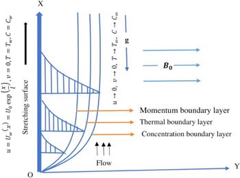
Consider mixed convection in a second-grade laminar, incompressible, steady, 2D, magnetized second-grade fluid flow over a sheet positioned along the $x$-axis in the vertical direction, although fluid in the domain $y\gt 0$ is constrained. It is also presumed that the sheet is stretched at an exponential rate $u={U}_{0}\exp \left(\tfrac{x}{l}\right)$, where ${U}_{0}$ is the reference velocity. Figure 1 demonstrates the geometrical configuration of the present flow.

Figure 1.

New window|Download| PPT slide
Figure 1.Flow over a hot vertical plate at temperature ${T}_{w}$ immersed in a fluid at temperature ${T}_{\infty }.$


The governing equations for
(1)$\begin{eqnarray}u=u\left(x,y\right),\,v=v\left(x,y\right),T=T\left(x,y\right),\,C=C\left(x,y\right),\end{eqnarray}$
are as follows:

continuity equation
(2)$\begin{eqnarray}\displaystyle \frac{\partial u}{\partial x}+\displaystyle \frac{\partial v}{\partial y}=0,\end{eqnarray}$
equation of motion
(3)$\begin{eqnarray}\begin{array}{c}\begin{array}{rcl}u\displaystyle \frac{{\rm{\partial }}u}{{\rm{\partial }}x}+v\displaystyle \frac{{\rm{\partial }}u}{{\rm{\partial }}y} & = & \vartheta \displaystyle \frac{{{\rm{\partial }}}^{2}u}{{\rm{\partial }}{y}^{2}}+\displaystyle \frac{{\alpha }_{1}}{{\rho }_{f}}\left(\displaystyle \frac{{\rm{\partial }}u}{{\rm{\partial }}x}\displaystyle \frac{{{\rm{\partial }}}^{2}u}{{\rm{\partial }}{y}^{2}}\right.\\ & & \begin{array}{c}\left.+\,u\displaystyle \frac{{{\rm{\partial }}}^{3}u}{{\rm{\partial }}x{\rm{\partial }}{y}^{2}}+\displaystyle \frac{{\rm{\partial }}u}{{\rm{\partial }}y}\displaystyle \frac{{{\rm{\partial }}}^{2}v}{{\rm{\partial }}{y}^{2}}+v\displaystyle \frac{{{\rm{\partial }}}^{3}u}{{\rm{\partial }}{y}^{3}}\right)\\ -\,\displaystyle \frac{\sigma {B}_{0}^{2}}{{\rho }_{f}}u+g{\beta }_{{\rm{T}}}\left(T-{T}_{\infty }\right)+g{\beta }_{{\rm{c}}}\left(C-{C}_{\infty }\right),\end{array}\end{array}\end{array}\end{eqnarray}$
energy equation
(4)$\begin{eqnarray}u\displaystyle \frac{\partial T}{\partial x}+v\displaystyle \frac{\partial T}{\partial y}={\alpha }_{f}\displaystyle \frac{{\partial }^{2}T}{\partial {y}^{2}}+\tau \left({D}_{{\rm{B}}}\displaystyle \frac{\partial C}{\partial y}\displaystyle \frac{\partial T}{\partial y}+\displaystyle \frac{{D}_{T}}{{T}_{\infty }}{\left(\displaystyle \frac{\partial T}{\partial y}\right)}^{2}\right),\end{eqnarray}$
nanoparticle volume fraction equation
(5)$\begin{eqnarray}u\displaystyle \frac{\partial C}{\partial x}+v\displaystyle \frac{\partial C}{\partial y}={D}_{{\rm{B}}}\displaystyle \frac{{\partial }^{2}C}{\partial {y}^{2}}+\displaystyle \frac{{D}_{T}}{{T}_{\infty }}\displaystyle \frac{{\partial }^{2}T}{\partial {y}^{2}}.\end{eqnarray}$
In the governing system $u$ and $v$ are the velocity components along the $x$- and $y$-directions, while $T$ and $C$ represent temperature and concentration variables, respectively, ${\rho }_{f}$ is the fluid density, $\sigma $ represents the electrical conductivity, $\vartheta $ is the kinematic viscosity, ${B}_{0}$ indicates the applied magnetic field, ${\alpha }_{1}$ is the second-grade fluid material parameter, $g$ is the gravitational acceleration, ${\beta }_{{\rm{T}}}$ and ${\beta }_{{\rm{c}}}$ are the thermal and concentration enlargement coefficients, respectively, $\tau $ describes the ratio between the nanoparticle’s heat capacity and the original fluid heat capacity, ${D}_{{\rm{B}}}$ represents the coefficient of Brownian diffusion, ${D}_{T}$ indicates the thermophoresis diffusion coefficient, ${C}_{\infty }$ and ${T}_{\infty }$ are upstream concentration and temperature, respectively, and $\alpha $ is thermal diffusivity.

The suitable boundary conditions for the considered flow problems are
(6)$\begin{eqnarray}\begin{array}{l}u={U}_{w}\left(x\right)={U}_{0}\exp \left(\displaystyle \frac{x}{l}\right),\,v=0,\,T={T}_{w}={T}_{\infty }\\ \,+\,{T}_{0}\exp \left(\displaystyle \frac{2x}{l}\right),\,C={C}_{w}={C}_{\infty }+{C}_{0}\exp \left(\displaystyle \frac{2x}{l}\right)\,{\rm{at}}\\ y=0,\end{array}\end{eqnarray}$

(7)$\begin{eqnarray}u\to 0,\,v\to 0,\,T\to {T}_{\infty },\,C\to {C}_{\infty }\,{\rm{as}}\,y\to \infty .\end{eqnarray}$

3. Non-similar analysis

We propose the following non-similarity transformations
(8)$\begin{eqnarray}\begin{array}{l}\eta =\sqrt{\displaystyle \frac{{U}_{0}}{2\vartheta l}}\exp \left(\displaystyle \frac{x}{2l}\right)y,\,{\rm{\xi }}=\exp \left(\displaystyle \frac{x}{l}\right),\,\\ u={U}_{0}\exp \left(\displaystyle \frac{x}{l}\right)\displaystyle \frac{\partial f\left(\xi ,\eta \right)}{\partial \eta },\,\\ v=-\sqrt{\displaystyle \frac{\vartheta {U}_{0}}{2l}}\,\left(f\left(\xi ,\eta \right)+2\xi \displaystyle \frac{\partial f\left(\xi ,\eta \right)}{\partial \xi }+\eta \displaystyle \frac{\partial f\left(\xi ,\eta \right)}{\partial \eta }\right)\exp \left(\displaystyle \frac{x}{2l}\right),\\ \theta \left(\xi ,\eta \right)=\displaystyle \frac{T-{T}_{\infty }}{{T}_{0}\exp \left(\tfrac{2x}{l}\right)},\,\phi \left(\xi ,\eta \right)=\displaystyle \frac{C-{C}_{\infty }}{{C}_{0}\exp \left(\tfrac{2x}{l}\right)}.\end{array}\end{eqnarray}$
These transformations identically satisfy the continuity equation (2). Substituting (8) into (3)-(7), we get the following system of dimensionless PDEs
(9)$\begin{eqnarray}\begin{array}{l}\displaystyle \frac{\alpha \xi \left(f+2\xi \tfrac{\partial f}{\partial \xi }\right)}{2}\displaystyle \frac{{\partial }^{4}f}{\partial {\eta }^{4}}-\alpha {\xi }^{2}\left(\displaystyle \frac{{\partial }^{2}f}{\partial \xi \partial \eta }\displaystyle \frac{{\partial }^{3}f}{\partial {\eta }^{3}}+\displaystyle \frac{{\partial }^{4}f}{\partial \xi \partial {\eta }^{3}}\displaystyle \frac{\partial f}{\partial \eta }\right.\\ \,-\,\left.\displaystyle \frac{{\partial }^{3}f}{\partial \xi \partial {\eta }^{2}}\displaystyle \frac{{\partial }^{2}f}{\partial {\eta }^{2}}\right)+2\xi \left(\displaystyle \frac{{\partial }^{2}f}{\partial \xi \partial \eta }\displaystyle \frac{\partial f}{\partial \eta }-\displaystyle \frac{{\partial }^{2}f}{\partial {\eta }^{2}}\displaystyle \frac{\partial f}{\partial \xi }\right)\\ \,=\,\displaystyle \frac{{\partial }^{3}f}{\partial {\eta }^{3}}+f\displaystyle \frac{{\partial }^{2}f}{\partial {\eta }^{2}}-2{\left(\displaystyle \frac{\partial f}{\partial \eta }\right)}^{2}-2\displaystyle \frac{{M}^{2}}{\xi }\displaystyle \frac{\partial f}{\partial \eta }\\ \,+\,\displaystyle \frac{\alpha \xi }{2}\left\{6\displaystyle \frac{{\partial }^{3}f}{\partial {\eta }^{3}}\displaystyle \frac{\partial f}{\partial \eta }-3{\left(\displaystyle \frac{{\partial }^{2}f}{\partial {\eta }^{2}}\right)}^{2}\right\}+2\lambda \left(\theta +N\phi \right),\end{array}\end{eqnarray}$

(10)$\begin{eqnarray}\begin{array}{l}\displaystyle \frac{{\partial }^{2}\theta }{\partial {\eta }^{2}}+Pr\left\{f\displaystyle \frac{\partial \theta }{\partial \eta }-4\theta \displaystyle \frac{\partial f}{\partial \eta }+{\xi }^{2}\left({N}_{b}\displaystyle \frac{\partial \theta }{\partial \eta }\displaystyle \frac{\partial \phi }{\partial \eta }+{N}_{t}{\left(\displaystyle \frac{\partial \theta }{\partial \eta }\right)}^{2}\right)\right\}\\ \,=\,2Pr\xi \left(\displaystyle \frac{\partial \theta }{\partial \xi }\displaystyle \frac{\partial f}{\partial \eta }-\displaystyle \frac{\partial f}{\partial \xi }\displaystyle \frac{\partial \theta }{\partial \eta }\right),\end{array}\end{eqnarray}$

(11)$\begin{eqnarray}\begin{array}{l}\displaystyle \frac{{\partial }^{2}\phi }{\partial {\eta }^{2}}+\displaystyle \frac{{N}_{t}}{{N}_{b}}\displaystyle \frac{{\partial }^{2}\theta }{\partial {\eta }^{2}}+{S}_{c}\left(f\displaystyle \frac{\partial \phi }{\partial \eta }-4\phi \displaystyle \frac{\partial f}{\partial \eta }\right)\\ \,=\,2\xi {S}_{c}\left(\displaystyle \frac{\partial \phi }{\partial \xi }\displaystyle \frac{\partial f}{\partial \eta }-\displaystyle \frac{\partial f}{\partial \xi }\displaystyle \frac{\partial \phi }{\partial \eta }\right).\end{array}\end{eqnarray}$
In the above equations, the magnetic parameter $\left(M\right),$ second-grade fluid parameter $(\alpha ),\,$ Richardson number $(\lambda ),$ ratio of mass and heat transfer Grashof numbers $(N),$ Brownian motion $\left(\,{N}_{b}\right),$ Prandtl number $(Pr),\,$ thermophoresis $({N}_{t}),$ and Schmidt number $({S}_{c})$, respectively, are defined as
(12)$\begin{eqnarray}\begin{array}{c}\begin{array}{c}{M}^{2}=\displaystyle \frac{\sigma {B}_{0}^{2}l}{{\rho }_{f}{U}_{0}},\,\alpha =\displaystyle \frac{{\alpha }_{1}{U}_{0}}{{\rho }_{f}\vartheta l},\,\lambda =\displaystyle \frac{g{\beta }_{{\rm{T}}}{T}_{0}l}{{U}_{0}^{2}},\\ N=\displaystyle \frac{g{\beta }_{{\rm{c}}}{C}_{0}l}{g{\beta }_{{\rm{T}}}{T}_{0}l},\,{N}_{b}=\displaystyle \frac{\tau {C}_{0}{D}_{{\rm{B}}}}{\vartheta },\\ Pr=\displaystyle \frac{\vartheta }{{\alpha }_{f}},\,{N}_{t}=\displaystyle \frac{\tau {D}_{T}{T}_{0}}{\vartheta {T}_{\infty }},\,{S}_{c}=\displaystyle \frac{\vartheta }{{D}_{{\rm{B}}}}.\,\end{array}\end{array}\end{eqnarray}$

4. First truncation system

By using a local similarity technique the terms containing a partial derivative with respect to $\xi $ are treated as approximately small and considered equal to zero. Therefore, equations (9)-(11) become
(13)$\begin{eqnarray}\begin{array}{l}{f}^{iv}-\displaystyle \frac{2}{\alpha \xi f}\left({f}^{\prime\prime\prime }+f{f}^{^{\prime\prime} }-2{f}^{{\prime} 2}-\displaystyle \frac{2{M}^{2}}{\xi }f^{\prime} \right.\\ +\,\left.\displaystyle \frac{\alpha \xi }{2}\left(6{f}^{\prime\prime\prime }f^{\prime} -3{f}^{{\prime\prime} 2}\right)+2\lambda \left(\theta +N\phi \right)\right)=0,\end{array}\end{eqnarray}$

(14)$\begin{eqnarray}\theta ^{\prime\prime} -Pr\left(4\theta f^{\prime} -f\theta ^{\prime} -{\xi }^{2}\left({N}_{b}\theta ^{\prime} \phi ^{\prime} +{N}_{t}{\theta }^{{\prime} 2}\right)\right)=0,\end{eqnarray}$

(15)$\begin{eqnarray}\phi ^{\prime\prime} +\displaystyle \frac{{N}_{t}}{{N}_{b}}\theta ^{\prime\prime} +{S}_{c}\left(f\phi ^{\prime} -4\phi f^{\prime} \right)=0.\end{eqnarray}$
The boundary conditions are
(16)$\begin{eqnarray}{f}^{{\prime} }\left(\xi ,0\right)=1,\,f\left(\xi ,0\right)=0,\,\theta \left(\xi ,0\right)=1,\,\phi \left(\xi ,0\right)=1.\end{eqnarray}$

(17)$\begin{eqnarray}f^{\prime} \left(\xi ,\infty \right)=0,\,f\left(\xi ,\infty \right)=0,\,\theta \left(\xi ,\infty \right)=0,\,\phi \left(\xi ,\infty \right)=0.\end{eqnarray}$

5. Second truncation system

For the second truncation system we considered
$\begin{eqnarray*}\displaystyle \frac{\partial f}{\partial \xi }=g,\,\displaystyle \frac{\partial \theta }{\partial \xi }=h,\,\displaystyle \frac{\partial \phi }{\partial \xi }=p.\,\,\,{\rm{and}}\,\displaystyle \frac{\partial g}{\partial \xi }=\displaystyle \frac{\partial h}{\partial \xi }=\displaystyle \frac{\partial p}{\partial \xi }=0.\end{eqnarray*}$


Equations (9)-(11) take the following form
(18)$\begin{eqnarray}\begin{array}{l}{f}^{iv}-\displaystyle \frac{2}{\alpha \xi \left(f+2\xi g\right)}\left({f}^{\prime\prime\prime }+f^{\prime} f^{\prime\prime} -2{f}^{{\prime} 2}-\displaystyle \frac{2{M}^{2}}{\xi }f^{\prime} \right.\\ +\,\displaystyle \frac{\alpha \xi }{2}\left(6{f}^{\prime\prime\prime }f^{\prime} -3{f}^{{\prime\prime} 2}\right.\left.+\,2\xi \left(g^{\prime} {f}^{\prime\prime\prime }+{g}^{\prime\prime\prime }f^{\prime} -g^{\prime\prime} f^{\prime\prime} \right)\right)\\ -\,\left.2\xi \left(g^{\prime} f^{\prime} -f^{\prime\prime} g\right)+2\lambda \left(\theta +N\phi \right)\right)=0,\end{array}\end{eqnarray}$

(19)$\begin{eqnarray}\begin{array}{l}{g}^{iv}-\displaystyle \frac{2}{{\left(\alpha \xi \left(f+2\xi g\right)\right)}^{2}}\left(\left(\alpha \xi \left(f+2\xi g\right)\right)\right.\\ \times \,\left(g\prime\prime\prime +g{f}^{{\prime\prime} }+f{g}^{{\prime\prime} }-4{f}^{^{\prime} }{g}^{^{\prime} }-\displaystyle \frac{2{M}^{2}}{{\xi }^{2}}\left({f}^{^{\prime} }-\xi {g}^{^{\prime} }\right)\right.\\ +\,\displaystyle \frac{\alpha }{2}\left.\left(6{f}^{\prime\prime\prime }{f}^{^{\prime} }-3{f}^{{\prime\prime} 2}+2\xi \left(5\left({g}^{^{\prime} }f\prime\prime\prime +{g}^{\prime\prime\prime }{f}^{^{\prime} }-{g}^{{\prime\prime} }{f}^{{\prime\prime} }\right)+\xi \left(2{g}^{^{\prime} }{g}^{\prime\prime\prime }-{g}^{{\prime\prime} 2}\right)\right)\right.\right)\\ \left.-\,2\left({g}^{^{\prime} }{f}^{^{\prime} }-{f}^{{\prime\prime} }g+\xi \left({g}^{{\prime} 2}-g{g}^{{\prime\prime} }\right)\right)+2\lambda \left(h+Np\right)\right)\\ -\,\alpha \left({f}^{\prime\prime\prime }+{f}^{^{\prime} }{f}^{{\prime\prime} }-2{f}^{{\prime} 2}-\displaystyle \frac{2{M}^{2}}{\xi }{f}^{^{\prime} }\right.\\ +\,\displaystyle \frac{\alpha \xi }{2}\left(6{f}^{\prime\prime\prime }{f}^{^{\prime} }-3{f}^{{\prime\prime} 2}+2\xi \left({g}^{^{\prime} }{f}^{\prime\prime\prime }+{g}^{\prime\prime\prime }{f}^{^{\prime} }-{g}^{{\prime\prime} }{f}^{{\prime\prime} }\right)\right)\\ \left.\left.-\,2\xi \left({g}^{^{\prime} }{f}^{^{\prime} }-{f}^{{\prime\prime} }g\right)+2\lambda \left(\theta +N\phi \right)\right)\left(f+5\xi g\right)\right)=0,\end{array}\end{eqnarray}$

(20)$\begin{eqnarray}{\theta }^{{\prime\prime} }-Pr\left(4\theta {f}^{^{\prime} }-f{\theta }^{^{\prime} }+2\xi \left(h{f}^{^{\prime} }-g{\theta }^{^{\prime} }\right)-{\xi }^{2}\left({N}_{b}{\theta }^{^{\prime} }{\phi }^{^{\prime} }+{N}_{t}{\theta }^{{\prime} 2}\right)\right)=0,\end{eqnarray}$

(21)$\begin{eqnarray}\begin{array}{l}{h}^{{\prime\prime} }-Pr\left(6h{f}^{^{\prime} }+4\theta {g}^{^{\prime} }-3g{\theta }^{^{\prime} }+f{h}^{^{\prime} }+2\xi \left(h{g}^{^{\prime} }-g{h}^{^{\prime} }-{N}_{b}{\theta }^{^{\prime} }{\phi }^{^{\prime} }-{N}_{t}{\theta }^{{\prime} 2}\right)\right.\\ \left.\,-\,{\xi }^{2}\left({N}_{b}{\theta }^{^{\prime} }{p}^{^{\prime} }+{N}_{b}{h}^{^{\prime} }{\phi }^{^{\prime} }+2{N}_{t}{\theta }^{^{\prime} }{h}^{^{\prime} }\right)\right)=0,\end{array}\end{eqnarray}$

(22)$\begin{eqnarray}{\phi }^{{\prime\prime} }={S}_{c}\left(4\phi {f}^{^{\prime} }-f{\phi }^{^{\prime} }+2\xi \left(p{f}^{^{\prime} }-g{\phi }^{^{\prime} }\right)\right)-\displaystyle \frac{{N}_{t}}{{N}_{b}}{\theta }^{{\prime\prime} },\end{eqnarray}$

(23)$\begin{eqnarray}{p}^{{\prime\prime} }={S}_{c}\left(6p{f}^{^{\prime} }+4\phi {g}^{^{\prime} }-3g{\phi }^{^{\prime} }-f{p}^{^{\prime} }+2\xi \left(p{g}^{^{\prime} }-g{p}^{^{\prime} }\right)\right)-\displaystyle \frac{{N}_{t}}{{N}_{b}}{h}^{{\prime\prime} }.\end{eqnarray}$
The boundary conditions are
(24)$\begin{eqnarray}{g}^{{\prime} }\left(0,\xi \right)=0,\,g\left(0,\xi \right)=0,\,h\left(0,\xi \right)=0,\,p\left(0,\xi \right)=0.\end{eqnarray}$

(25)$\begin{eqnarray}{g}^{{\prime} }\left(\infty ,\xi \right)=0,\,g\left(\infty ,\xi \right)=0,\,h\left(\infty ,\xi \right)=0,\,p\left(\infty ,\xi \right)=0.\end{eqnarray}$
The parameters of physical interest, such as the friction coefficient ${C}_{{\rm{f}}},$ the local Nusselt number $Nu$ and the Sherwood number $Sh$ are defined as,
(26)$\begin{eqnarray}{C}_{{\rm{f}}}=\displaystyle \frac{2{\tau }_{wx}}{\rho {U}_{w}^{2}\left(x\right)},\,=\displaystyle \frac{x{q}_{w}(x)}{K({T}_{w}-{T}_{\infty })},\,Sh=\displaystyle \frac{x{j}_{w}}{{D}_{{\rm{B}}}({C}_{w}-{C}_{\infty })},\end{eqnarray}$
where the wall skin friction ${\tau }_{wx},$ ${\rm{heat}}\,\mathrm{flux}\,{q}_{w}$ and mass flux ${j}_{w}$ are expressed as
(27)$\begin{eqnarray}{\tau }_{wx}=\mu {\left(\displaystyle \frac{\partial u}{\partial y}\right)}_{y=0},\,{q}_{w}=-K{\left(\displaystyle \frac{\partial T}{\partial y}\right)}_{y=0},\,{j}_{w}=-{D}_{{\rm{B}}}{\left(\displaystyle \frac{\partial C}{\partial y}\right)}_{y=0}.\end{eqnarray}$
Using (27) in (26) we get,
(28)$\begin{eqnarray}\begin{array}{r}\begin{array}{c}{\left({Re}\right)}^{\tfrac{1}{2}}{C}_{{\rm{f}}}=\sqrt{\displaystyle \frac{2}{\xi }}{f}^{{'}{'}}\left(0\right),\,R{e}^{-\tfrac{1}{2}}N{u}_{x}=-\,{\rm{ln}}\,\xi \sqrt{\displaystyle \frac{\xi }{2}}{\theta }^{{'}}\left(0\right),\\ \,R{e}^{-\tfrac{1}{2}}Sh=-\,{\rm{ln}}\,\xi \sqrt{\displaystyle \frac{\xi }{2}}{\phi }^{{'}}\left(0\right).\end{array}\end{array}\end{eqnarray}$

6. Results and discussion

The interpretation of solutions regarding the impacts of the different dimensionless quantities on ${f}^{{\prime} }\left(\eta \right),$ $\theta \left(\eta \right)$ and $\phi \left(\eta \right)$ are presented in this section. The variation in the numerical data of the friction coefficient $(\,{C}_{{\rm{f}}}),$ Nusselt number ($Nu$) and Sherwood number ($Sh$) for numerous values of involved quantities are depicted in this tabular form. The Nusselt number is the ratio of convective to conductive heat transfer, and the Sherwood number is defined as the ratio of the convective mass transfer to the mass diffusivity at a boundary in a fluid. Large values of the Nusselt number show pre-eminence of convection of heat transfer over conduction and small values of the Nusselt number indicate that poor convection occurs. So the Nusselt number indicates the dominant heat transfer phenomenon of the system. Graphical analysis of the velocity, temperature and concentration fields are conferred to explain the current non-similar model.

Table 1 shows the range of governing parameters in which graphical solutions of velocity, temperature and concentration profiles reveal stable behavior. Table 2 depicts the impacts of the magnetic parameter $\left(M\right),$ Richardson number $(\lambda ),$ second-grade fluid parameter $(\alpha )$ and ratio of mass and heat transfer Grashof numbers $(N)$ on the local skin friction. We perceive that the friction coefficient decreases marginally as $M$ increases, while the coefficient of skin friction increases due to increases in the values of $\alpha ,\,\lambda $ and $N.$


Table 1.
Table 1.The range of defined parameters for a stable solution.

$M$	$\alpha $	$\lambda $	$N$	$Pr$	$Nb$	$Nt$	$Sc$
1-20	1	0.1	0.1	10	0.1	0.1	0.1
2	1-8	5	0.1	10	0.1	0.1	0.1
2	1	0-20	0.1	10	0.1	0.1	0.1
2	1	2	0-16	10	0.1	0.1	0.1
2	2	7	1	1-35	1	1	1
4	4	4	2	7	0.1-2	0.5	1
4	4	5	1	7	0.4	0-1	1
1	2	5	1	7	0.4	0.4	0.3-50

New window|CSV


Table 2.
Table 2.Numerical data for the skin friction coefficient $R{e}_{x}^{\tfrac{1}{2}}{C}_{{\rm{f}}}$ for various parameters.

$M$	$\alpha $	$\xi $	$\lambda $	$N$	${N}_{b}$	${N}_{t}$	${S}_{c}$	$Pr$	$-R{e}_{x}^{\tfrac{1}{2}}{C}_{{\rm{f}}}$
1	1.5	2.5	0.1	0.1	0.1	0.1	0.1	10	0.663 583 4713
2	1.5	2.5	0.1	0.1	0.1	0.1	0.1	10	0.856 293 1308
3	1.5	2.5	0.1	0.1	0.1	0.1	0.1	10	1.225 811 0306
4	1.5	2.5	0.1	0.1	0.1	0.1	0.1	10	1.574 931 1745
2	1	1.5	1.5	0.1	0.1	0.1	0.1	10	1.830 895 0187
2	2	1.5	1.5	0.1	0.1	0.1	0.1	10	1.444 299 1125
2	3	1.5	1.5	0.1	0.1	0.1	0.1	10	1.210 097 2603
2	4	1.5	1.5	0.1	0.1	0.1	0.1	10	1.060 750 1270
2	1	1.5	1	0.1	0.1	0.1	0.1	10	1.029 614 1067
2	1	1.5	2	0.1	0.1	0.1	0.1	10	0.989 847 5139
2	1	1.5	3	0.1	0.1	0.1	0.1	10	0.924 498 0245
2	1	1.5	4	0.1	0.1	0.1	0.1	10	0.874 504 9428
2	1	2	2	0.1	0.1	0.1	0.1	10	1.265 880 9749
2	1	2	2	0.2	0.1	0.1	0.1	10	1.216 799 9095
2	1	2	2	0.3	0.1	0.1	0.1	10	1.164 759 5975
2	1	2	2	0.4	0.1	0.1	0.1	10	1.125 926 6318

New window|CSV

Table 3 displays the local Nusselt number values for the various governing parameter values. It is established that the rate of heat transfer on the wall increases due to the increase in ${N}_{b}.$ It is also shown that uplifting the values of the parameters $Pr\,$ and ${N}_{t}$ resulted in a decline in the numeric values of the local Nusselt number.


Table 3.
Table 3.The local Nusselt number $R{e}_{x}^{-\tfrac{1}{2}}N{u}_{x}$ for various parameters.

$M$	$\alpha $	$\xi $	$\lambda $	$N$	${N}_{b}$	${N}_{t}$	${S}_{c}$	$Pr$	$-R{e}_{x}^{-\tfrac{1}{2}}N{u}_{x}$
4	2	0.01	5	0.1	0.1	0.1	0.1	8	0.264 954 9335
4	2	0.01	5	0.1	0.1	0.1	0.1	10	0.312 707 1600
4	2	0.01	5	0.1	0.1	0.1	0.1	12	0.362 955 6961
4	2	0.01	5	0.1	0.1	0.1	0.1	15	0.438 384 2125
4	4	0.01	5	2	0.2	0.5	1	7	0.235 524 6848
4	4	0.01	5	2	0.3	0.5	1	7	0.206 545 0969
4	4	0.01	5	2	0.4	0.5	1	7	0.191 251 8247
4	4	0.01	5	2	0.6	0.5	1	7	0.165 460 3569
4	4	0.01	5	1	0.1	0.2	0.1	10	0.255 267 7573
4	4	0.01	5	1	4	0.4	0.1	10	0.293 119 1975
4	4	0.01	5	1	4	0.6	0.1	10	0.302 495 9839
4	4	0.01	5	1	4	0.8	0.1	10	0.308 375 4409

New window|CSV

Table 4 describes the impact of governing parameters on the local Sherwood number. The table shows that for increasing ${N}_{t}\,{\rm{and}}\,{S}_{c}$ values, the local Sherwood coefficient decreases.


Table 4.
Table 4.Numerical data for the local Sherwood number $R{e}_{x}^{-\tfrac{1}{2}}Sh$ for various parameters.

$M$	$\alpha $	$\xi $	$\lambda $	$N$	${N}_{b}$	${N}_{t}$	${S}_{c}$	$Pr$	$-R{e}_{x}^{-\tfrac{1}{2}}Sh$
2	2	0.01	5	1	0.4	0.4	0.2	7	0.127 830 7934
2	2	0.01	5	1	0.4	0.4	0.4	7	0.141 073 9103
2	2	0.01	5	1	0.4	0.4	0.6	7	0.294 137 7066
2	2	0.01	5	1	0.4	0.4	0.8	7	0.307 232 1177
2	2	0.01	5	1	0.2	0.4	0.1	7	0.102 663 3317
2	2	0.01	5	1	0.3	0.4	0.1	7	0.101 851 7903
2	2	0.01	5	1	0.4	0.4	0.1	7	0.093 584 0243
2	2	0.01	5	1	0.5	0.4	0.1	7	0.095 747 2218
2	2	0.01	5	1	0.4	0.1	0.1	7	0.075 010 4120
2	2	0.01	5	1	0.4	0.2	0.1	7	0.084 432 5427
2	2	0.01	5	1	0.4	0.3	0.1	7	0.087 396 3154
2	2	0.01	5	1	0.4	0.4	0.1	7	0.093 584 0243

New window|CSV

Whereas the local Sherwood number increases with the increasing values of ${N}_{b}.$

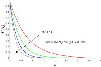
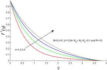
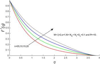
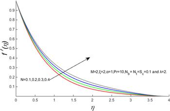
Figures 2-5 demonstrate the velocity profiles for different parameters like $M,$ $\alpha ,$ $\delta$and $N.$ The consequence of an applied magnetic field $M$ in the transverse direction on flow over a stretching sheet is shown in figure 2. It is observed that the increase in magnetic field reduces the fluid velocity. In general, an increase in the applied magnetic field in the transverse direction produces the Lorentz force which opposes the flow. We observed that the Lorentz force effect reduces the flow of the velocity profile. Figure 3 indicates that the fluid flow increases with increasing $\alpha$, thus thickening the boundary velocity layer. Figures 4 and 5 give an insight into the effect of ${\rm{\lambda }}$ and $N$ on velocity. From figure 4 it is conspicuous that the velocity profile increases with increasing values of ${\rm{\lambda }}.$ Figure 5 indicates that the velocity profile increases with the increasing values of $N$ (ratio of mass and heat transfer Grashof numbers) due to the buoyancy effect.

Figure 2.

New window|Download| PPT slide
Figure 2.$f^{\prime} \left(\eta \right)$ for several values of $ \mbox{``} M\mbox{''}.$

Figure 3.

New window|Download| PPT slide
Figure 3.$f^{\prime} \left(\eta \right)$ for several values of '$\alpha$’.

Figure 4.

New window|Download| PPT slide
Figure 4.$f^{\prime} \left(\eta \right)$ for several values of 'λ’.

Figure 5.

New window|Download| PPT slide
Figure 5.$f^{\prime} \left(\eta \right)$ for several values of 'N’.


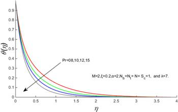
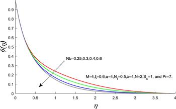
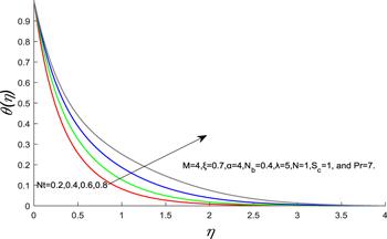
Figure 6 reveals that the effect of increasing the $Pr$ is a decrease in the temperature profile. The ratio of momentum diffusivity and thermal diffusivity is specified by the Prandtl number. So, it is clear that the rise in $Pr$ decreases the thickness of the thermal boundary layer. Figure 7 expresses the dimensionless temperature for several values of ${N}_{b}.$ It shows that due to a rise in the values of ${N}_{b},$ the temperature profile decreases. From figure 8 it is seen that the temperature profile rises with the increasing values of the thermophoresis parameter ${N}_{t}.$

Figure 6.

New window|Download| PPT slide
Figure 6.$\theta \left(\eta \right)$ for several values of '$Pr$’.

Figure 7.

New window|Download| PPT slide
Figure 7.$\theta \left(\eta \right)$ for several values of '${N}_{b}$’.

Figure 8.

New window|Download| PPT slide
Figure 8.$\theta \left(\eta \right)$ for several values of '${N}_{t}$’.


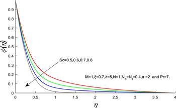
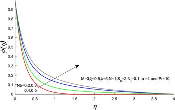
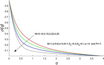
Figure 9 shows the influence of the Schmidt number ${S}_{c}$ on the mass concentration profile. It is seen that a rise in ${S}_{c}$ leads to a reduction in the concentration boundary layer thickness. Figure 10 explains the impact of the Brownian motion parameter ${N}_{b}$ on the mass concentration profile. It is evident from the figure that the concentration profile rises with the upsurge in the values of ${N}_{b}.$ The influence of the thermophoresis parameter ${N}_{t}$ on the concentration profile is illustrated in figure 11. It is perceived that the concentration profile decreases with the increase in ${N}_{t}.$

Figure 9.

New window|Download| PPT slide
Figure 9.$\phi \left(\eta \right)$ for several values of '${S}_{c}$’.

Figure 10.

New window|Download| PPT slide
Figure 10.$\phi \left(\eta \right)$ for several values of '${N}_{b}$’.

Figure 11.

New window|Download| PPT slide
Figure 11.$\phi \left(\eta \right)$ for several values of '${N}_{t}$’.

7. Conclusions

In this research non-similar modeling is performed for second-grade magnetic nanofluid flow over a vertical surface which is stretching at an exponential rate. Non-similar solutions are obtained through local non-similarity via bvp4c. The important results are mentioned below.• The velocity profile is increased by the increase in $N,$ $\delta$and $\alpha$, while the velocity profile decreases as a result of the increase in $M.$
• The temperature profile is increased due to the increase in ${N}_{t}$, although the temperature profile decreases due to the increase in ${N}_{b}$ and ${\rm{\Pr }}.$
• The increase in the value ${N}_{b}$ leads to the rise in the volumetric concentration profile, while the opposite is true for ${S}_{c}$ and ${N}_{t}.$
• Local skin friction increases due to the increase in the values of $\alpha ,\,\lambda $ and $N$ and slightly decreases as the values of the $M$ increase.
• It is observed that the local Nusselt number upsurges against the ${N}_{b}$, whereas it declines by uplifting the ${\rm{\Pr }}$ and ${N}_{t}$ parameters.
• The local Sherwood number decreases with the increase in ${N}_{t}\,{\rm{and}}\,{S}_{c}$, but the effect is the reverse for ${N}_{b}.$

Reference View Option By original order
By published year
By cited within times
By Impact factor

[1]Sakiadis B C 1961Boundary layer behavior on continuous solid surfaces: II. The boundary layer on a continuous flat surface
AlChE J. 7 221 225
DOI:10.1002/aic.690070211 [Cited within: 1]

[2]Erickson L E, Fan L T, Fox V G 1966Heat and mass transfer on moving continuous flat plate with suction or injection
Ind. Eng. Chem. Fundam. 5 19 25
DOI:10.1021/i160017a004 [Cited within: 1]

[3]Crane L J 1970Flow past a stretching plate
Z. Angew. Math. Phys. ZAMP 21 645 647
DOI:10.1007/BF01587695 [Cited within: 2]

[4]Gupta P S, Gupta A S 1977Heat and mass transfer on a stretching sheet with suction or blowing
Can. J. Chem. Eng. 55 744 746
DOI:10.1002/cjce.5450550619 [Cited within: 1]

[5]Rajagopal K R, Na T Y, Gupta A S 1984Flow of a viscoelastic fluid over a stretching sheet
Rheol. Acta 23 213 215
DOI:10.1007/BF01332078 [Cited within: 1]

[6]Bujurke N M, Biradar S N, Hiremath P S 1987Second-order fluid flow past a stretching sheet with heat transfer
Z. Angew. Math. Phys. ZAMP 38 653 657
DOI:10.1007/BF00946345 [Cited within: 1]

[7]Magyari E, Keller B 1999Heat and mass transfer in the boundary layers on an exponentially stretching continuous surface
J. Phys. D: Appl. Phys. 32 577 585
DOI:10.1088/0022-3727/32/5/012 [Cited within: 1]

[8]Elbashbeshy E M A 2001Heat transfer over an exponentially stretching continuous surface with suction
Arch. Mech. 53 643 651
[Cited within: 1]

[9]Partha M K, Murthy P V S N, Rajasekhar G P 2005Effect of viscous dissipation on the mixed convection heat transfer from an exponentially stretching surface
Heat Mass Transfer 41 360 366
DOI:10.1007/s00231-004-0552-2 [Cited within: 1]

[10]Khan S K, Sanjayanand E 2005Viscoelastic boundary layer flow and heat transfer over an exponential stretching sheet
Int. J. Heat Mass Transfer 48 1534 1542
DOI:10.1016/j.ijheatmasstransfer.2004.10.032 [Cited within: 1]

[11]Xu H, Liao S J, Pop I 2007Series solutions of unsteady three-dimensional MHD flow and heat transfer in the boundary layer over an impulsively stretching plate
Eur. J. Mech. B 26 15 27
DOI:10.1016/j.euromechflu.2005.12.003 [Cited within: 1]

[12]Khan S K 2006Heat transfer in a viscoelastic fluid flow over a stretching surface with heat source/sink, suction/blowing and radiation
Int. J. Heat Mass Transfer 49 628 639
DOI:10.1016/j.ijheatmasstransfer.2005.07.049 [Cited within: 1]

[13]Bataller R C 2007Viscoelastic fluid flow and heat transfer over a stretching sheet under the effects of a non-uniform heat source, viscous dissipation and thermal radiation
Int. J. Heat Mass Transfer 50 3152 3162
DOI:10.1016/j.ijheatmasstransfer.2007.01.003 [Cited within: 1]

[14]Tan Y, Liao S J 2007Series solution of three-dimensional unsteady laminar viscous flow due to a stretching surface in a rotating fluid
J. Appl. Mech. 74 1011 1018
DOI:10.1115/1.2723816 [Cited within: 1]

[15]Sajid M, Hayat T 2008Influence of thermal radiation on the boundary layer flow due to an exponentially stretching sheet
Int. Commun. Heat Mass Transfer 35 347 356
DOI:10.1016/j.icheatmasstransfer.2007.08.006 [Cited within: 1]

[16]Sekhar G N, Chethan A S 2012Flow and heat transfer of an exponential stretching sheet in Boussinesq-Stokes suspension
Int. J. Math. Archive 3 1978 1984
DOI:10.36884/jafm.7.01.19473 [Cited within: 1]

[17]Siddheshwar P G, Sekhar G N, Chethan A S 2014MHD flow and heat transfer of an exponential stretching sheet in a Boussinesq-Stokes suspension
J. Appl. Fluid Mech. 7 169 176
DOI:10.36884/jafm.7.01.19473 [Cited within: 1]

[18]Ramzan M, Bilal M, Farooq U, Chung J D 2016Mixed convective radiative flow of second grade nanofluid with convective boundary conditions: an optimal solution
Results in Physics 6 796 804
DOI:10.1016/j.rinp.2016.10.011 [Cited within: 1]

[19]Rasheed A, Anwar M S 2019Interplay of chemical reacting species in a fractional viscoelastic fluid flow
J. Mol. Liq. 273 576 588
DOI:10.1016/j.molliq.2018.10.028 [Cited within: 1]

[20]Muhammad T 2020Significance of heat generation/absorption in magnetohydrodynamic flow by an unsteady stretching curved surface
Multidiscipline Model. Mater. Struct. 17 35 47
DOI:10.1108/MMMS-11-2019-0203 [Cited within: 1]

[21]Ahmad M, Muhammad T, Ahmad I, Aly S 2020Time-dependent 3D flow of viscoelastic nanofluid over an unsteady stretching surface
Physica A 551C 124004
DOI:10.1016/j.physa.2019.124004 [Cited within: 1]

[22]Jamil B, Anwar M S, Rasheed A, Irfan M 2020MHD Maxwell flow modeled by fractional derivatives with chemical reaction and thermal radiation
Chin. J. Phys. 67 512 533
DOI:10.1016/j.cjph.2020.08.012 [Cited within: 1]

[23]Irfan M, Anwar M S, Rashid M, Waqas M, Khan W A 2020Arrhenius activation energy aspects in mixed convection Carreau nanofluid with nonlinear thermal radiation
Appl. Nanosci. 10 4403 4413
DOI:10.1007/s13204-020-01498-5 [Cited within: 1]

[24]Ames W F 1965 Nonlinear Partial Differential Equations in Engineering New York Academic
[Cited within: 1]

[25]Bluman G W 1974Applications of the general similarity solution of the heat equation to boundary-value problems
Q. Appl. Math. 31 403 415
DOI:10.1090/qam/427829 [Cited within: 1]

[26]Cantwell B 2002 Introduction to Symmetry Analysis Paperback with CD-ROM Vol. 29 Cambridge Cambridge University Press


[27]Azad H, Mustafa M T, Arif A F M 2010Analytic solutions of initial-boundary-value problems of transient conduction using symmetries
Appl. Math. Comput. 215 4132 4140
DOI:10.1016/j.amc.2009.12.016

[28]Ovsiannikov L V E 2014 Group Analysis of Differential Equations New York Academic


[29]Farooq U, Hayat T, Alsaedi A, Liao S J 2015Series solutions of non-similarity boundary layer flows of nano-fluids over stretching surfaces
Numer. Algorithms 70 43 59
DOI:10.1007/s11075-014-9934-9 [Cited within: 1]

[30]Sparrow E M, Yu H S 1971Local non-similarity thermal boundary-layer solutions
J. Heat Transfer. 93 328 334
DOI:10.1115/1.3449827 [Cited within: 1]

[31]Hayat T, Saif R S, Ellahi R, Muhammad T, Ahmad B 2017Numerical study of boundary-layer flow due to a nonlinear curved stretching sheet with convective heat and mass conditions
Results in Physics 7 2601 2606
DOI:10.1016/j.rinp.2017.07.023 [Cited within: 1]

[32]Zhang C, Wang D, Xiang S, Han Y, Peng X 2017Numerical investigation of heat transfer and pressure drop in helically coiled tube with spherical corrugation
Int. J. Heat Mass Transfer 113 332 341
DOI:10.1016/j.ijheatmasstransfer.2017.05.108 [Cited within: 1]

[33]Ray A K, Vasu B, Murthy P V S N, Gorla R S 2020Non-similar solution of Eyring-Powell fluid flow and heat transfer with convective boundary condition: Homotopy Analysis Method
Int. J. Appl. Comput. Math. 6 16
DOI:10.1007/s40819-019-0765-1 [Cited within: 1]

[34]Farooq U, Ijaz M A, Khan M I, Isa S S P M, Lu D C 2020Modeling and non-similar analysis for Darcy-Forchheimer-Brinkman model of Casson fluid in a porous media
Int. Commun. Heat Mass Transfer 119 104955
DOI:10.1016/j.icheatmasstransfer.2020.104955 [Cited within: 1]