Cheng-Fu Mu(穆成富)^,1, Da-Li Zhang(张大立)^,1Department of physics, Huzhou University, Huzhou 313000, Zhejiang, China

First author contact: ¹ Authors to whom any correspondence should be addressed.
Received:2019-12-23Revised:2020-01-22Accepted:2020-01-23Online:2020-04-22

Fund supported:

*National Natural Science Foundation of China.11947410 National Natural Science Foundation of China.11147148 National Natural Science Foundation of China.U1832139 Natural Science Foundation of Zhejiang Province.LY19A050002

Abstract
Level structure and electromagnetic transitions in ⁹⁸Mo have been investigated on the basis of the proton-neutron interacting boson model (IBM-2) by considering the energy difference between neutron boson ϵ_ν and proton boson ϵ_π. The results are compared with the recent experimental data and it is observed that they are in good agreement. In particular, the strongest M1 transition from ${2}_{5}^{+}$ state to ${2}_{2}^{+}$ can be well reproduced, from which one can determine the ${2}_{5}^{+}$ as an mixed-symmetry (MS) state. We have calculated the electric monopole strength ${\rho }^{2}(E0,{0}_{2}^{+}\to {0}_{1}^{+})$, and our result agrees with the experimental one. The calculation indicates that shape coexistence and MS states are simultaneously well described using IBM-2.
Keywords： shape coexistence;mixed-symmetry state;IBM-2;E2 and M1 transitions


PDF (286KB)MetadataMetricsRelated articlesExportEndNote|Ris|BibtexFavorite
Cite this article
Cheng-Fu Mu(穆成富), Da-Li Zhang(张大立). A unified description of shape coexistence and mixed-symmetry states in ⁹⁸Mo using IBM-2^*. Communications in Theoretical Physics, 2020, 72(5): 055302- doi:10.1088/1572-9494/ab770a

1. Introduction

The molybdenum isotopes have rich nuclear structures and have been studied both experimentally and theoretically over many years, for example, for ⁹²Mo and ⁹⁴Mo [1–3] and ⁹⁶Mo and ⁹⁸Mo [4–9]. The theoretical methods include the variation-after-projection (VAP) calculations in conjunction with Hartree-Bogoliubov (HB) ansatz applied to A=100–108 molybdenum isotopes [10], the triaxial projected shell model (TPSM) approach to the band structures for neutron-rich ^102–108Mo [11], and algebraic model IBM [12–16]. One of the greatest interests that attract physicists lies in the shape-related topics, such as shape coexistence, shape evolution and shape phase transition from the even–even spherical magic-N-nucleus ⁹²Mo to deformed nucleus ¹⁰⁸Mo along the chain of Mo isotopes [17–19].

Shape coexistence has been observed in many parts of the nuclear chart and related theoretical works were carried out for a long time [20–26]. In or near the shell or sub-shell closures, the monopole interaction of nuclear force tends to stabilize the nucleus into a spherical shape. However, in around mid-shell regions, the correlation energy gain tends to drive the nucleus into a deformed shape. The competition between the two opposite actions is the resource of the shape coexistence phenomenon [27]. For ⁹⁴Mo, the 0⁺ state at 1.742 MeV is the third excited state above the ground state. But for ⁹⁶Mo, the 0⁺ state at 1.148 MeV is the second excited state. The 0⁺ state at 0.735 MeV becomes the first excited state in ⁹⁸Mo. The appearance of low-lying 0⁺ state provides a clue for the coexistence of different shapes in some Mo isotopes [6, 27, 28]. The theoretical description of shape coexistence is mainly based on shell model and the mean field theory. In the shell model, the intruder configurations originated from the valence nucleons across the shell or sub-shell gaps are responsible for the mechanism of shape coexistence. In the mean field theory, one can calculate the potential energy surface (PES) and different shapes correspond to a different minimum in the PES. The interacting boson model (IBM) provides another tool to deal with the shape coexistence. The different shapes correspond to the different algebraic structure group of IBM, therefore, one can discuss the shape-related phenomenon by investigating the group structure. It has been found that there exists three dynamical symmetries characterized by the first algebra in the chain originating from group structure, that is, U(5), SU(3), O(6), corresponding to spherical, axially deformed, and γ-unstable shapes, respectively [29–37].

The IBM-2, which makes a distinction between neutrons and protons, predicts the existence of MS states, which are not completely symmetric under the exchange of the neutron-proton bosons [38, 39]. The totally symmetric states under this exchange are called full symmetry (FS) states. The experimental signatures of MS states are characterized by the strong M1 transitions between FS and MS states with transition matrix element of about one μ_N and weakly collective E2 transitions between FS and MS states, which strengths can only reach a few percent of $B(E2,{2}_{1}^{+}\to {0}_{1}^{+})$. In addition, there exists strongly collective E2 transitions between MS states, with typical strength comparable to the collective E2 transitions between symmetric states [40, 41].

The properties of ⁹⁸Mo nucleus have been discussed in many previous papers. In [8], the authors employed the IBM-1 to describe the experimental data available at that time and found that the triaxial ground state and the prolate first excited state coexist in ⁹⁸Mo. In [12], the authors discussed the effect of configuration mixing on Mo isotopes, but they only calculated the E(2) transitions and did not consider the M(1) transitions and MS states. Both of these two works were based on the previous experiments, the data were not enough at that time. Recently, the excited low-spin states in ⁹⁸Mo were studied in γγ angular correlation experiment [4], their new experimental data show that both shape coexistence and MS states exist in ⁹⁸Mo. In [28], the authors found the the IBM-2 could reproduce the correct excitation energy levels of the Mo isotopes without resorting to the configuration mixing by taking the energy of neutron boson ϵ_ν different from that of proton boson ϵ_π. In this study, the purpose is to apply the method of [28] to describe the properties of shape coexistence and MS states in ⁹⁸Mo in a unified framework.

The paper is structured as follows. In section 2 we briefly introduce the theoretical framework of IBM-2 model and its parameters fitted in our calculation. In section 3, we discuss the calculated results of the low-lying levels in comparison with its corresponding experimental data. In section 4, we investigate the electromagnetic transition probabilities including $E2,M1$ and E0 properties. Finally, a conclusion is given in section 5.

2. Theoretical model

The microscopic picture of the IBM originates from the idea that the collective fermion pairs of valence nucleons play an important role in the nuclear structure, where only pairs coupled to L=0 (s boson) and L=2 (d boson) are considered. The connection between the IBM and shell model was first pointed out in [42–44]. This is one of the reasons for the success of IBM. In the IBM-2, one assumes that the valence neutrons or protons outside a closed shell can be treated as neutron or proton bosons. For a full description of IBM-2, we refer the reader to [45]. The explicit expression of the Hamiltonian in this calculation is as follows(1)$\begin{eqnarray}\begin{array}{rcl}\hat{H} & = & {\varepsilon }_{\pi }{\hat{n}}_{{d}_{\pi }}+{\varepsilon }_{\nu }{\hat{n}}_{{d}_{\nu }}+{\kappa }_{\pi \nu }{\hat{Q}}_{\pi }\cdot {\hat{Q}}_{\nu }\\ & & +{\omega }_{\pi \nu }{\hat{L}}_{\pi }\cdot {\hat{L}}_{\nu }+{\omega }_{\nu \nu }{\hat{L}}_{\nu }\cdot {\hat{L}}_{\nu }+{\hat{M}}_{\pi \nu }\\ & & +\displaystyle \frac{1}{2}\sum _{\rho =\pi ,\nu }\sum _{L=0,2,4}{\left(2L+1\right)}^{\tfrac{1}{2}}{c}_{\rho }^{(L)}{\left({[{d}_{\rho }^{\dagger }{d}_{\rho }^{\dagger }]}^{(L)}\cdot {[{\tilde{d}}_{\rho }{\tilde{d}}_{\rho }]}^{(L)}\right)}_{0}^{(0)},\,\end{array}\end{eqnarray}$where ${\hat{n}}_{d\rho }={d}_{\rho }^{\dagger }\cdot \tilde{{d}_{\rho }}\,$ is the d-boson number operator, and ${\hat{Q}}_{\rho }={\left({s}_{\rho }^{\dagger }{\tilde{d}}_{\rho }+{d}_{\rho }^{\dagger }{s}_{\rho }\right)}^{(2)}+{\chi }_{\rho }{\left({d}_{\rho }^{\dagger }{\tilde{d}}_{\rho }\right)}^{(2)}\,$ the quadrupole operator for the neutron (ρ=ν) and proton (ρ=π), respectively. The parameters ϵ_π, ϵ_ν denote the energy of d bosons relative to the s bosons. χ_π(χ_ν) represents the quadrupole structure parameter of proton (neutron) bosons, having only a minor effect on the excitation energy but contributing a lot to the electromagnetic properties. For U(5)-like nuclei, their spectrum is dominated by the value of ϵ_ρ, which is relatively much larger than other parameters. For O(6)-like nuclei, the value of κ_πν large in comparison with ϵ_ρ characterizes the main properties of their spectrum. The fourth and fifth terms on the right-hand side of equation (1) stand for the dipole proton-neutron and neutron-neutron interaction, respectively. The angular momentum operator is defined as $\hat{{L}_{\rho }}=\sqrt{10}{[{d}_{\rho }^{\dagger }\cdot \tilde{{d}_{\rho }}]}^{(1)}$. The sixth term represents the Majorana interaction, having expression as ${\hat{M}}_{\pi \nu }={\lambda }_{2}{\left({s}_{\pi }^{\dagger }{d}_{\nu }^{\dagger }-{s}_{\nu }^{\dagger }{d}_{\pi }^{\dagger }\right)}^{(2)}\cdot {\left({s}_{\pi }{\tilde{d}}_{\nu }-{s}_{\nu }{\tilde{d}}_{\pi }\right)}^{(2)}$ $+\,{\sum }_{k=\mathrm{1,3}}{\lambda }_{k}{\left({d}_{\pi }^{\dagger }{d}_{\nu }^{\dagger }\right)}^{(k)}\cdot {\left({\tilde{d}}_{\pi }{\tilde{d}}_{\nu }\right)}^{(k)}$. The Majorana parameters λ_k (k=1, 2, 3) only influence the excitation energies of states having MS components, which will be fixed by the known experimental data. The last term is the interaction between like bosons. The E2 and M1 transition operators are written as(2)$\begin{eqnarray}{\hat{T}}^{(E2)}={e}_{\pi }{\hat{Q}}_{\pi }+{e}_{\nu }{\hat{Q}}_{\nu },\ \end{eqnarray}$(3)$\begin{eqnarray}{\hat{T}}^{(M1)}=\sqrt{3/4\pi }({g}_{\nu }{\hat{L}}_{\nu }+{g}_{\pi }{\hat{L}}_{\pi }),\ \end{eqnarray}$where the e_ρ and g_ρ are the effective quadrupole charges and the gyromagnetic ratios, respectively.

The reduced E2 transition probability $B(E2)$ is obtained by(4)$\begin{eqnarray}B(E2,J\to J^{\prime} )=\displaystyle \frac{1}{2J+1}| \langle J^{\prime} \parallel {\hat{T}}^{(E2)}\parallel J\rangle {| }^{2},\end{eqnarray}$with J and $J^{\prime} $ being the initial and final spin angular momenta, respectively. The reduced M1 transition probability $B(M1)$ reads(5)$\begin{eqnarray}B(M1,J\to J^{\prime} )=\displaystyle \frac{1}{2J+1}| \langle J^{\prime} \parallel {\hat{T}}^{(M1)}\parallel J\rangle {| }^{2}.\end{eqnarray}$The monopole strength ρ² in the IBM-2 is defined as follows [46](6)$\begin{eqnarray}{\rho }^{2}(E0,J\to J^{\prime} )=\displaystyle \frac{{Z}^{2}}{{e}^{2}{R}^{4}}{[{\beta }_{0\nu }\langle J^{\prime} \parallel {\hat{n}}_{d\nu }\parallel J\rangle +{\beta }_{0\pi }\langle J^{\prime} \parallel {\hat{n}}_{d\pi }\parallel J\rangle ]}^{2},\end{eqnarray}$where $R=1.2{A}^{1/3}$ fm, and ${\beta }_{0\pi (\nu )}$ is the proton (neutron) monopole boson effective charge in unit of efm², the d-boson number operator ${\hat{n}}_{d\rho }$ is the same as in equation (1).More detailed explanation about the Hamiltonian and the transition operators can be seen in [45]. The Hamiltonian was diagonalized using NPBOS code [47].

We choose the doubly closed-shell ${}_{\ 50}^{100}{\mathrm{Sn}}_{50}$ as the inert core in this paper. For nucleus ${}_{42}^{98}$Mo${}_{56},{N}_{\pi }=4$ hole-like proton bosons from the Z=50 closed shell and N_ν=3 particle-like neutron bosons from the N=50 closed shell can be easily determined. Generally, the IBM-2 calculations assumed ε_π=ε_ν for the sake of restricting the number of free parameters. However as pointed out in [28], the valence neutrons and protons do not fill the same orbitals when they are added to the inert core. Therefore, the excitation energy of neutron d boson ${\epsilon }_{\nu }$ should be different from that of proton d boson ε_π. This is our staring point in this calculation.

The interaction between like proton bosons for the Mo isotopes can be negligible, the parameters ${c}_{\pi }^{(0,2,4)}$ is set to zero. We use ${c}_{\nu }^{(2)}=0$, ${c}_{\nu }^{(4)}=0.0$ to minimize the number of free parameters in the Hamiltonian (1). By a least-square fitting to the experimental data for ⁹⁸Mo, we obtain the final IBM-2 parameters in our analysis: ϵ_ν=0.501 MeV, ϵ_π= 0.815 MeV, ${\kappa }_{\pi \nu }=-0.06\,\mathrm{MeV}$, ω_πν=0.1 MeV, ω_νν= 0.14 MeV, χ_π= −χ_ν=0.6, λ₁=1.318 MeV, λ₂= 0.072 MeV, and λ₃= 0.47 MeV ${c}_{\nu }^{(0)}=-0.49$.

3. The energy level structure

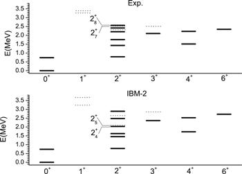
Figure 1 shows the experimental and calculated energy levels. The explicit results are listed in table 1. As discussed above, by noting that the energy of neutron boson ϵ_ν is not equal to that of proton boson ϵ_π, namely ${\varepsilon }_{\nu }\ne {\varepsilon }_{\pi }$, we can reproduce the ordering of ${0}_{1}^{+},{0}_{2}^{+},{2}_{1}^{+},{2}_{2}^{+}$ and ${4}_{1}^{+}$ states very well. Especially, the level energies of the first four states are almost equal to the corresponding experimental data. The energy of ${2}_{2}^{+}$ state is slightly lower than ${4}_{1}^{+}$ state, they constitutes a pair, the ${0}_{2}^{+}$ state is far from them, this is a character of γ-soft spectrum.

Figure 1.

New window|Download| PPT slide
Figure 1.Spectrum for ⁹⁸Mo. Experimental(upper panel) and calculated(lower panel) energy levels (in units of MeV) are depicted for positive-parity low-spin states. The MS states having the quantum number F_max-1 are labeled with dashed lines. The experimental data are adopted from [4–6].



Table 1.
Table 1.Experimental level energies reported in [4–6]) are compared to the results from IBM-2 calculations near Z=N=50 doubly shell closure.

	${E}_{\mathrm{Expt}}$	${E}_{\mathrm{IBM}-2}$	F	R
${0}_{1}^{+}$	0.000	0.000	2	99.2
${0}_{2}^{+}$	0.735	0.735	2	68.7
${1}_{1}^{+}$	3.258	3.243	1	55.2
${1}_{2}^{+}$	3.405	3.668	1	51.5
${2}_{1}^{+}$	0.787	0.787	2	96.3
${2}_{2}^{+}$	1.432	1.453	2	94.3
${2}_{3}^{+}$	1.758	1.628	2	65.8
${2}_{4}^{+}$	2.207	2.031	2	68.0
${2}_{5}^{+}$	2.333	2.068	1	57.6
${2}_{6}^{+}$	2.419	2.479	2	60.8
${2}_{7}^{+}$	2.526	2.649	1	54.7
${2}_{8}^{+}$	2.562	2.886	2	76.1
${3}_{1}^{+}$	2.105	2.364	2	94.0
${3}_{2}^{+}$	2.485	2.845	1	53.8
${4}_{1}^{+}$	1.510	1.727	2	82.8
${4}_{2}^{+}$	2.224	2.523	2	83.8
${6}_{1}^{+}$	2.343	2.722	2	61.1

New window|CSV

A new quantum number called F-spin first introduced by Arima et al can give a good description of MS states [42]. The FS states have the maximum eigenvalue of F-spin, namly ${F}_{\max }=({N}_{\pi }+{N}_{\nu })/2$, where N_ν (${N}_{\pi }$) is the total number of neutron (proton) bosons. The MS states are characterized by other eigenvalues: $F={F}_{\max }-1$, ${F}_{\max }-2,\,\ldots ,\,{F}_{\min }=\left|{N}_{\pi }-{N}_{\nu }\right|/2$ [48]. An important quantity indicating the F-spin nature of a given state $| s\rangle $ is the ratio R defined by(7)$\begin{eqnarray}R=\langle s\parallel {F}^{2}\parallel s\rangle /{F}_{\max }({F}_{\max }+1),\ \end{eqnarray}$where(8)$\begin{eqnarray}| s\rangle =\alpha | {F}_{\max }\rangle +\beta | {F}_{\max }-1\rangle ,\hspace{5mm}{\alpha }^{2}+{\beta }^{2}=1,\ \end{eqnarray}$then we obtain(9)$\begin{eqnarray}\langle s\parallel {F}^{2}\parallel s\rangle ={\alpha }^{2}{F}_{\max }({F}_{\max }+1)+{\beta }^{2}{F}_{\max }({F}_{\max }-1).\ \end{eqnarray}$R=1 for an FS state. The smaller the R is, the lower the F-spin becomes. Therefore, R indicates the main component of a state wavefunction in the F-spin space. If R is less than sixty percent, one can consider this state as an MS state. Table 1 shows that the ${1}_{1}^{+},{1}_{2}^{+},{2}_{5}^{+},{2}_{7}^{+},{3}_{2}^{+}$ are some candidates for MS states. The experimental energy of ${2}_{5}^{+}$ state lies at 2.333 MeV, the calculated energy at 2.068 MeV is a little lower than the experimental value. The lowest MS state is the ${2}_{5}^{+}$ state. Further identification of MS states needs to analyze the information about the electromagnetic transitions, we will discuss these properties later.

The energy ratio ${R}_{4/2}=E({4}_{1}^{+})/E({2}_{1}^{+})$ is an ideal observable of measuing the extent of quadrupole deformation, which has different characteristic values for three kinds of typical nuclei: R_4/2=2 for spherical nuclei, R_4/2=2.5 for γ-unstable nuclei and R_4/2=3.33 for rigid rotors. The experimental value of R_4/2 is 1.92, the calculation gives R_4/2=2.19, both of them indicate that it is a near-harmonic U(5) spectrum. But only the R_4/2 value can not uniquely determine the shape character of a nucleus, one needs other information such as the electromagnetic transition properties to give more decisive discussions. Figure 1 shows that the experimental levels can be perfectly described by IBM-2 including the MS states.

4. The electromagnetic transitions

In this study, we let the effective quadrupole charge of neutron boson e_ν=0 for simplicity, and determine the effective charge e_π by fitting to the experimental result of $B(E2,{2}_{1}^{+}\to {0}_{1}^{+})=21.4$ W.u. for ⁹⁸Mo nucleus. At last, we obtain the e_π=0.1211 eb. For the boson g factors, we take the naked values g_ν=0 and g_π=1.0 μ_N.

In tables 2 and 3, we compare the calculated electromagnetic $B(E2)$ and $B(M1)$ transition strengths for ⁹⁸Mo with the recent experimental values. Tables 2 and 3 indicate that most of the calculated B(E2) transition strengths can reproduce the experimental results very well. For the $B(M1)$ transitions, we list the calculated results that have the correspondence with the experimental data. In table 3, we use the relative values of B(E2) transition strengths as reported in [5]. For U(5)-like nuclei, E2 transition strengths must obey the selection rule $\bigtriangleup {n}_{d}=0,\pm 1$. But M1 transitions can only occurs between states which have the same d boson number n_d [49]. In the O(6) limit the ${0}_{2}^{+}$ state is the head of a band with τ=3 and $\sigma ={\sigma }_{{\rm{m}}}$, the selection rules only allow the transition between ${2}_{2}^{+}$ state and ${0}_{2}^{+}$ state , but this transition is forbidden in the U(5) limit. As shown in table 2, the calculated transition $B(E2,{2}_{2}^{+}\to {0}_{2}^{+})=0.513$ W.u. agrees with the experimental one ${2.5}_{-6}^{+8}$ W.u. within the experimental uncertainty. This displays that ⁹⁸Mo has the O(6) feature. The experimental value of $B(E2,{2}_{1}^{+}\to {0}_{2}^{+})$ transition is too large and needs further theoretical investigation.


Table 2.
Table 2.Experimental E2 and M1 transition strengths for ⁹⁸Mo are compared to the calculated ones, where E2 strengths are given in unit of W.u., and the M1 transition are given in unit of ${\mu }_{N}^{2}$. The experimental data are adopted from [4–6].

${J}_{i}^{\pi }\to {J}_{f}^{\pi }$	$B(E2)$		$B(M1)$
	Expt.	IBM-2	Expt.	IBM-2
${2}_{1}^{+}\to {0}_{1}^{+}$	21.4	21.4
${2}_{1}^{+}\to {0}_{2}^{+}$	280(40)	0.250
${2}_{2}^{+}\to {0}_{1}^{+}$	${1.0}_{-1}^{+2}$	0.251
${2}_{2}^{+}\to {0}_{2}^{+}$	${2.5}_{-6}^{+8}$	0.513
${2}_{2}^{+}\to {2}_{1}^{+}$	${47.8}_{-100}^{+132}$	23.93	0.0119(2)	0.019 99
${2}_{3}^{+}\to {0}_{2}^{+}$	${7.8}_{-34}^{+286}$	9.27
${2}_{3}^{+}\to {2}_{1}^{+}$	${3.2}_{-16}^{+134}$	2.73	0.0179(4)	0.111
${2}_{3}^{+}\to {2}_{2}^{+}$	${4.7}_{-23}^{+189}$	1.12
${2}_{4}^{+}\to {2}_{1}^{+}$	1.7(2)	0.45	${0.059}_{-6}^{+7}$	0.0599
${2}_{5}^{+}\to {2}_{2}^{+}$	${1.6}_{-4}^{+8}$	0.635	${0.153}_{-41}^{+87}$	0.1467
${2}_{7}^{+}\to {2}_{2}^{+}$	0.0043(6)	0.06	0.018(12)	0.005 14
${4}_{1}^{+}\to {2}_{1}^{+}$	${49.1}_{-4.5}^{+5.5}$	33.64
${6}_{1}^{+}\to {4}_{1}^{+}$	10.1(4)	34.10

New window|CSV


Table 3.
Table 3.Same as table 2, but normalized with respect to the largest $B(E2)$ transition strength of initial states ${3}_{1}^{+}$ and ${4}_{2}^{+}$, respectively. The experimental data are taken from [5].

${J}_{i}^{\pi }\to {J}_{f}^{\pi }$	$B(E2)$
	Expt.	IBM-2
${3}_{1}^{+}\to {2}_{1}^{+}$	0.04(3)	0.004
${3}_{1}^{+}\to {2}_{2}^{+}$	1	1
${3}_{1}^{+}\to {4}_{1}^{+}$	$\lt 0.40$	0.24
${4}_{2}^{+}\to {2}_{1}^{+}$	0.04(1)	0.01
${4}_{2}^{+}\to {2}_{2}^{+}$	0.88(11)	1.45
${4}_{2}^{+}\to {4}_{1}^{+}$	1	1

New window|CSV

Another observable characterizing the shape character is $B(E2,{4}_{1}^{+}\to {2}_{1}^{+})$ transition. The calculated value of $B(E2,{4}_{1}^{+}\to {2}_{1}^{+})$ is 33.64 W.u., a little lower than the experimental value of ${49.1}_{-4.5}^{+5.5}$ W.u.. As shown in table 4, the calculated ratio ${B}_{4/2}={\text{}}B(E2,{4}_{1}^{+}\to {2}_{1}^{+})/{\text{}}B(E2,{2}_{1}^{+}\to {0}_{1}^{+})=1.57$ closely matches the corresponding experimental value of 2.29, although the recent experimental uncertainty is large. For $N\to \infty $, the well-known results are B_4/2=2 for U(5) limit and 10/7 for O(6) limit. For the finite number of boson N=7, the IBM gives B_4/2=1.71 for the U(5) limit and B_4/2=1.34 for the O(6) limit [49, 50]. Both the calculated and experimental values of B_4/2 indicate that ⁹⁸Mo nucleus appears to be closer to the U(5) limit, but the calculation contains a little more O(6) components.


Table 4.
Table 4.The characteristic $B(E2)$ ratios for low-lying states in the three dynamical limits (taken from the [49, 50]). Both of the experimental and calculated values are listed.

	$\tfrac{B(E2,{4}_{1}^{+}\to {2}_{1}^{+})}{B(E2,{2}_{1}^{+}\to {0}_{1}^{+})}$	$\tfrac{B(E2,{2}_{2}^{+}\to {0}_{1}^{+})}{B(E2,{2}_{2}^{+}\to {2}_{1}^{+})}$	$\tfrac{B(E2,{2}_{2}^{+}\to {2}_{1}^{+})}{B(E2,{2}_{1}^{+}\to {0}_{1}^{+})}$	$\tfrac{B(E2,{4}_{1}^{+}\to {2}_{1}^{+})}{B(E2,{2}_{2}^{+}\to {2}_{1}^{+})}$
U(5)	1.71	0.011	1.4	1.0
SU(3)	1.34	0.70	0.02	6.93
O(6)	1.34	0.07	0.79	1.84
Exp.	2.29	0.02	2.23	1.03
IBM-2	1.57	0.01	1.12	1.41

New window|CSV

The computed E2 transition strength of $B(E2,{2}_{2}^{+}\,\to {2}_{1}^{+})\,=23.93$ W.u. is in agreement with the experimental value ${47.8}_{-100}^{+132}$ W.u. within the experimental uncertainty. In order to investigate the shape character, we introduce another characteristic ratio ${B}_{2/2}={\text{}}B(E2,{2}_{2}^{+}\to {2}_{1}^{+})/{\text{}}B(E2,{2}_{1}^{+}\to {0}_{1}^{+})$. The experimental value gives B_2/2=2.23. But the available experimental data have some uncertainties in ⁹⁸Mo. Our calculation obtains B_2/2=1.12. Both the calculated and experimental values of B_2/2 imply that ⁹⁸Mo nucleus demonstrates the U(5) character. Table 4 also gives the results of $B(E2,{2}_{2}^{+}\to {0}_{1}^{+})/B(E2,{2}_{2}^{+}\to {2}_{1}^{+})$ and $B(E2,{4}_{1}^{+}\,\to {2}_{1}^{+})/B(E2,{2}_{2}^{+}\to {2}_{1}^{+})$, which reveal similar behavior as above.

The E0 transition strength ${\rho }^{2}(E0)$ can provide the valuable information on shape coexistence [51]. Therefore, we calculate the ${\rho }^{2}(E0,{0}_{2}^{+}\to {0}_{1}^{+})$ transition probability in order to further understand the structure character in ⁹⁸Mo. Because the E0 operator is proportional to ${\hat{n}}_{d}$, there are no E0 transitions in the U(5) limit [37]. We adopt the same parameters ${\rho }_{0\nu }=0.25$ efm² and ${\rho }_{0\pi }=0.10$ efm² as in [46]. The calculated transition strength ${\rho }^{2}(E0,{0}_{2}^{+}\to {0}_{1}^{+})=0.0159$. The experimental value of ${\rho }^{2}(E0,{0}_{2}^{+}\to {0}_{1}^{+})$ is 0.027(2) [6]. The theoretical calculation agrees with the experimental value. Combining with the discussion on the level structure, we conclude that the character of shape coexistence can be well described in the framework of IBM-2 in ⁹⁸Mo.

From table 2, it is shown that the agreement between the theoretical calculation and the experimental data for M1 transitions appears to be satisfactory. Especially, the strongest M1 transition from ${2}_{5}^{+}$ state to ${2}_{2}^{+}$ can be well reproduced. The calculated $B(E2,{2}_{2}^{+}\to {2}_{1}^{+})$ and $B(E2,{2}_{4}^{+}\to {2}_{1}^{+})$ are almost equal to the experimental values. Both the experimental $B(E2,{2}_{5}^{+}\to {2}_{2}^{+})$ value and the calculated one demonstrate that this is a weakly collective E2 transition. Combining with the R value in table 1, one can determine the ${2}_{5}^{+}$ state has an MS character. This is the first MS state in ⁹⁸Mo. In the same way, the ${2}_{7}^{+}$ state is also an MS state.

5. Conclusion

In summary, we have calculated the low-lying levels and E2 and M1 electromagnetic transitions for a number of transitions in ⁹⁸Mo using IBM-2 by considering the energy difference of neutron boson and proton boson, ${\varepsilon }_{\nu }\ne {\varepsilon }_{\pi }$. The comparison between the recent experimental data and calculated ones shows that they are in good agreement. In particular, the strongest M1 transition from ${2}_{5}^{+}$ state to ${2}_{2}^{+}$ state can be well reproduced. The calculation indicates that ${2}_{5}^{+}$ and ${2}_{7}^{+}$ states belong to the mixed-symmetry states. We also calculated the electric monopole strength ${\rho }^{2}(E0,{0}_{2}^{+}\to {0}_{1}^{+})$, the result agrees with the experimental data. Our calculation indicates that shape coexistence and MS states can be simultaneously described very well in the framework of IBM-2.

Reference View Option By original order
By published year
By cited within times
By Impact factor

[1]Gupta Y K et al. 2018 Phys. Rev. C 97 064323
DOI:10.1103/PhysRevC.97.064323 [Cited within: 1]

[2]Wieser M E De Laeter J R 2007 Phys. Rev. C 75 055802
DOI:10.1103/PhysRevC.75.055802

[3]Fransen C et al. 2003 Phys. Rev. C 67 024307
DOI:10.1103/PhysRevC.67.024307 [Cited within: 1]

[4]Thomas T et al. 2016 Nucl. Phys. A 947 203
DOI:10.1016/j.nuclphysa.2015.12.010 [Cited within: 5]

[5]Thomas T et al. 2013 Phys. Rev. C 88 044305
DOI:10.1103/PhysRevC.88.044305 [Cited within: 2]

[6]Rusev G et al. 2005 Phys. Rev. Lett. 95 062501
DOI:10.1103/PhysRevLett.95.062501 [Cited within: 5]

[7]Lesher S R et al. 2007 Phys. Rev. C 75 034318
DOI:10.1103/PhysRevC.75.034318

[8]Zielińska M et al. 2002 Nucl. Phys. A 712 3
DOI:10.1016/S0375-9474(02)01169-7 [Cited within: 1]

[9]Youngblood D H Lui Y W Krishichayan Button J Bonasera G Shlomo S 2015 Phys. Rev. C 92 014318
DOI:10.1103/PhysRevC.92.014318 [Cited within: 1]

[10]Sawhney N Bharti A Khosa S K 2002 Pramana—J. Phys. 59 585
DOI:10.1007/s12043-002-0070-z [Cited within: 1]

[11]Bhat G H Sheikh J A Sun Y Palit R 2016 Nucl. Phys. A 947 127
DOI:10.1016/j.nuclphysa.2015.12.006 [Cited within: 1]

[12]Sambataro M Molnár G 1982 Nucl. Phys. A 376 201
DOI:10.1016/0375-9474(82)90060-4 [Cited within: 2]

[13]Mu C F Zhang D L 2018 Sci. China-Phys. Mech. Astron. 61 012011
DOI:10.1007/s11433-017-9106-5

[14]Mu C F Zhang D L 2018 Chin. Phys. Lett. 35 062101
DOI:10.1088/0256-307X/35/6/062101

[15]Zhang D L Ding B G 2014 Sci. China-Phys. Mech. Astron. 57 447
DOI:10.1007/s11433-014-5394-4

[16]Zhang J F AL-Khudair H F Long G L Zhu S J Ruan D 2002 Commun. Theor. Phys. 37 335
DOI:10.1088/0253-6102/37/3/335 [Cited within: 1]

[17]Skalski J Mizutori S Nazarewicz W 1997 Nucl. Phys. A 617 282
DOI:10.1016/S0375-9474(97)00125-5 [Cited within: 1]

[18]Abusara H Ahmad S Othman S 2017 Phys. Rev. C 95 054302
DOI:10.1103/PhysRevC.95.054302

[19]Federman P Pittel S 1979 Phys. Rev. C 20 820
DOI:10.1103/PhysRevC.20.820 [Cited within: 1]

[20]Wood J L Heyde K Nazarewicz W Huyse M van Duppen P 1992 Phys. Rep. 215 101
DOI:10.1016/0370-1573(92)90095-H [Cited within: 1]

[21]Cejnar P Jolie J Casten R F 2010 Rev. Mod. Phys. 82 2155
DOI:10.1103/RevModPhys.82.2155

[22]Sabri H Jahangiri Z Mohammadi M A 2016 Nucl. Phys. A 946 11
DOI:10.1016/j.nuclphysa.2015.11.001

[23]Zhang D L Mu C F 2018 Chin. Phys. C 42 034101
DOI:10.1088/1674-1137/42/3/034101

[24]Zhang D L Mu C F 2016 Chin. Phys. Lett. 33 102102
DOI:10.1088/0256-307X/33/10/102102

[25]Ren Z Z 2002 Phys. Rev. C 65 051304
DOI:10.1103/PhysRevC.65.051304

[26]Bai Z J Fu X M Jiao C F Xu F R 2015 Chin. Phys. C 39 094101
DOI:10.1088/1674-1137/39/9/094101 [Cited within: 1]

[27]Heyde K Wood J L 2011 Rev. Mod. Phys. 83 1467
DOI:10.1103/RevModPhys.83.1467 [Cited within: 2]

[28]Dejbakhsh H Latypov D Ajupova G Shlomo S 1992 Phys. Rev. C 46 2326
DOI:10.1103/PhysRevC.46.2326 [Cited within: 4]

[29]Van Isacker P Heyde K Jolie J Sevrin A 1986 Ann. Phys. (NY) 171 253
DOI:10.1016/0003-4916(86)90002-3 [Cited within: 1]

[30]Otsuka T 1992 Hyperfine Interact. 75 23
DOI:10.1007/BF02398961

[31]Caprio M A Iachello F 2005 Ann. Phys. 318 454
DOI:10.1016/j.aop.2005.02.003

[32]Liu Y X Mu L Z Wei H Q 2006 Phys. Lett. B 633 49
DOI:10.1016/j.physletb.2005.11.018

[33]Zhang Y Pan F Liu Y X Luo Y A Draayer J P 2017 Phys. Rev. C 96 034323
DOI:10.1103/PhysRevC.96.034323

[34]Zhang Y Hou Z F Liu Y X 2007 Phys. Rev. C 76 011305(R)
DOI:10.1103/PhysRevC.76.011305

[35]Long G L Liu Y X Sun H Z 1990 J. Phys. G 16 813
DOI:10.1088/0954-3899/16/6/006

[36]Liu Y X Long G L Sun H Z 1990 J. Phys. G 17 877
DOI:10.1088/0954-3899/17/6/010

[37]Leviatan A Shapira D 2016 Phys. Rev. C 93 051302(R)
DOI:10.1103/PhysRevC.93.051302 [Cited within: 2]

[38]Long G L Li Y S Tu C C Tian L Ji H Y Zhu S J Zhao E G Liu F Y Zhang J F Ruan D 2002 Commun. Theor. Phys. 37 75
DOI:10.1088/0253-6102/37/1/75 [Cited within: 1]

[39]AL-Khudair F H Long G L 2002 Commun. Theor. Phys. 37 699
DOI:10.1088/0253-6102/37/6/699 [Cited within: 1]

[40]Pietralla N von Brentano P Lisetskiy A F 2008 Prog. Part. Nucl. Phys. 60 225
DOI:10.1016/j.ppnp.2007.08.002 [Cited within: 1]

[41]Heyde K von Neumann-Cosel P Richter A 2010 Rev. Mod. Phys. 82 2365
DOI:10.1103/RevModPhys.82.2365 [Cited within: 1]

[42]Arima A Otsuka T Iachello F Talmi I 1977 Phys. Lett. B 66 205
DOI:10.1016/0370-2693(77)90860-7 [Cited within: 2]

[43]Otsuka T Arima A Iachello F Talmi I 1978 Phys. Lett. B 76 139
DOI:10.1016/0370-2693(78)90260-5

[44]Otsuka T 1981 Nucl. Phys. A 368 244
DOI:10.1016/0375-9474(81)90685-0 [Cited within: 1]

[45]Iachello F Arima A 1987 The Interacting Boson Model Cambridge Cambridge University Press
[Cited within: 2]

[46]Giannatiempo A Nannimi A Sona P 1991 Phys. Rev. C 44 2326
DOI:10.1103/PhysRevB.44.2326 [Cited within: 2]

[47]Otsuka T Yoshida N 1985 Program NPBOS. JAER-M Report, No. 85–094 1 (unpublished)
[Cited within: 1]

[48]Sun H Z Long G L Zhang J Y Han Q Z 1998 Commun. Theor. Phys. 29 411
DOI:10.1088/0253-6102/29/3/411 [Cited within: 1]

[49]Casten R F Warner D D 1988 Rev. Mod. Phys. 60 389
DOI:10.1103/RevModPhys.60.389 [Cited within: 3]

[50]Stachel J Van Isacker P Heyde K 1982 Phys. Rev. C 25 650
DOI:10.1103/PhysRevC.25.650 [Cited within: 2]

[51]Wood J L Zganjar E F De Coster C Heyde K 1999 Nucl. Phys. A 651 323
DOI:10.1016/S0375-9474(99)00143-8 [Cited within: 1]