 ,1,2,?, Kai Kang3, Shao-Jing Qin1, Chui-Lin Wang4
Corresponding authors: ? E-mail:fengdl@itp.ac.cn
Received:2018-11-23Online:2019-04-1
| Fund supported: |

Abstract
Keywords:
PDF (361KB)MetadataMetricsRelated articlesExportEndNote|Ris|BibtexFavorite
Cite this article
De-Long Feng, Kai Kang, Shao-Jing Qin, Chui-Lin Wang. Unified Description on Behavior of Lyapunov Exponent for 1-D Anderson Model Near Band Center *. [J], 2019, 71(4): 463-467 doi:10.1088/0253-6102/71/4/463
1 Introduction
Since Anderson's pioneering work on the interplay of quantum mechanics and disorder, localized system has been extensively studied over the past several decades.[1] Arising naturally in real systems, disorder could influence the transport property of electrons in solids, which show fascinating behaviors.[2-6] It was demonstrated that, in one-dimensional system, arbitrary small disorder strength will cause exponential localization of all the eigenstates in the band, which was confirmed by numerical simulation methods.[7-8] Among these studies, most efforts are focused on the discrete Hamiltonian,where $\epsilon_i$ is the on-site energy and $t_{ji}$ is the hopping energy from the $i$-th site to the $j$-th site. Varying from system to system, we can basically divide them into diagonal or off-diagonal and correlated or non-correlated disorder systems.[9-10] In this paper, we aim at one-dimensional system with diagonal and uncorrelated disorder in which only hoppings between the nearest sites are considered.
For previous models, it was found that the Lyapunov exponent behaves anomalously near
the band center,[11] which is deviated from Thouless formula.[12] The perturbation method has been applied to deal with this mysterious region in the weak or strong disorder limits.[13-15] Derrida and Gardner developed a disorder expansion method for weak disorder in Ref. [14], which recovered the anomaly near band center and band edge and predicted that similar anomaly exists in the vicinity of $E=2\cos\alpha\pi$, with $\alpha$ to be a rational number. Then it was confirmed in Ref. [16], where they obtained the Lyapunov exponent in two limiting cases around band center,
where $K(1/\sqrt2)$ is the complete elliptic function of the first kind, $E$ and $\sigma^2$ are the energy and disorder strength. Due to its sensitivity to energy and disorder strength, general analytical treatment to the whole neighborhood of band center has not been found yet. An analytical expression will be provided to relate the above two limiting cases in this work.
As discussed above, analytical formula performs well in the anomalous and traditional area respectively. Although it seems hard to connect them by a unified description, numerical calculation indicates that it could be possible to give formula except the band edge anomalous region.[17] In this work, by making use of the parametrization method proposed in a previous work,[18] we develop a new approach to obtain the invariant distribution coincided with the result given by Hamiltonian map method in Ref. [19]. This paper is organized as follows. In Sec. 2, we briefly review the parametrization method. In Sec. 3, by expanding the integral equation in terms of $E$ and $\sigma^2$, we derive a corresponding differential equation and invariant distribution. Then, the solution of this equation is used to obtain information in two limiting cases. In Sec. 4, a Padé approximation formula is given to describe the behavior of Lyapunov exponent for the whole neighborhood of band center.
2 Parametrization Method
We start by introducing the parametrization method in this section for the Schr?dinger equation of one-dimensional diagonal disorder Anderson system,The energy $E$ of an electron and the on-site energy ${\epsilon_i}$ of disorder system have been rescaled by the nearest neighbor hopping energy. $\{\epsilon_i\}$ are independent to each other and obey an identical distribution $p_\epsilon (\epsilon)$. In this study we assume that the random potential $\epsilon_i$ with a zero mean $<\epsilon>=0$, a nonzero variance $<\epsilon^2>=\sigma^2$, and an even distribution $p_\epsilon (-\epsilon) = p_\epsilon (\epsilon)$. For this purpose we use a standard distribution for on-site energy in our calculation,
The Schr?dinger equation can be rewritten in transfer matrix $ T_i$ as
As the authors performed in Ref. [18], we define the total transfer matrix $ M_L={ T_L}{ T_{L-1}}\ldots{ T_1}$, and parametrize it by two real parameters $\theta_L$ and $\lambda_L$.
where $ M_L^t$ is the transpose matrix of $ M_L$, and $ U(\theta_L)$ is
Utilizing the definition of $ M_{L}$ and $ M_{L+1}$, we obtain the recursion relation of $\theta_L$,
This recursion relation gives the exact integral equation for the stationary distribution function $\rho(\theta)$ of the random number $\theta_L$,
here $\theta_1$ is a function of $\theta$, $\tan\theta_1=E-\epsilon-{1}/{\tan\theta}$.
The Lyapunov exponent is the average of $(1/2) (\lambda_{L+1}-\lambda_{L})$, where $\lambda_{L}$ is defined in Eq. (6). $\gamma$ can be expressed by a normalized $\rho(\theta)$ in
It is equivalent to the formula $\gamma=\int \rho(\theta)\ln|\tan\theta|$ used in Refs. [13--14]. This integral equation and Lyapunov exponent are valid for all energies and disorder strengths.[18] We will use Eq. (10) in weak disorder and band center case at the last part of next section, as it can be expanded in terms of $\sigma^2$ and $E$ because of the direct relation to both distribution $p_{\epsilon}(\epsilon)$ and energy $E$.
When the variance $\sigma^2\rightarrow 0$, the distribution of $\theta$ is determined only by the distribution of $\theta_1$. The distribution of random potential becomes a delta function and it yields
Equation (11) gives the equation that the distribution function has to satisfy in the limiting case $\sigma^2 \to 0$. The solution of this equation is $\rho(\theta)=1/(1-({E}/{2})\sin 2\theta)$ for in-band energies.
In the limit $\sigma^2 \to 0$, if we consider next the band center limit $E\rightarrow 0$, Eq. (11) reduces to
It shows that if any distribution function satisfies $\rho(\theta)=\rho(\theta-{\pi}/{2})$, it may be a stationary distribution. There are many distributions under this symmetry. Then $\gamma$ is not uniquely defined, and this is not true for a disordered system. Such a degenerate phenomenon of $\rho(\theta)$ distribution has been discussed in Ref. [13]. It is the mathematical reason for the zero energy anomaly. At any $E=2\cos\alpha\pi$ with $\alpha$ to be a rational number, however, anomaly in $\gamma$ could rise in orders higher than $\sigma^2$, as a recent study[19] demonstrated. We will go to the next order of $\sigma^2$ for the exact integration equation Eq. (9) to resolve the unique $\rho(\theta)$ distribution under $E\to 0$ in next section.
3 $E/\sigma^2$ Dependence of Zero Energy Anomaly
In this section we write out the differential equation of distribution from the exact integration equation Eq. (9) in weak disorder for band center anomaly, formulate its solution, and expand the Lyapunov exponent $\gamma$ to the leading corrections for $\sigma^2/E \to 0$ and $\sigma^2/E \to \infty$.We approach the solution for band center by iterating this recursive integration equation twice
where $\tan\theta_1=E-\epsilon_1-{1}/{\tan\theta}$, and $\tan\theta_2=E-\epsilon_2-{1}/{\tan\theta_1}$. Then it is possible to calculate the stationary distribution in the limits $E\rightarrow 0$, $\sigma^2\rightarrow 0$. Since $\theta_2$ will be sufficiently close to $\theta$, $\rho(\theta_2)$ can be expanded around $\theta$, and the integration equation can be written into a differential equation of $\rho(\theta)$.
We expand Eq. (13) in powers of $E$ and $\sigma^2$
Let us neglect higher order terms of $\sigma^2$ and $E$. Then by defining $x={E}/{\sigma^2}$, we get
Equation (15) is in agreement with the result obtained in previous studies, for example the one obtained by Hamiltonian map method in Ref. [20-21].
The normalized distribution obtained as the solution of Eq. (15) in this study is
where $N(x)$ is the normalization factor. We include a factor ${ 2\sqrt2 x}/{1-e^{-\sqrt2 \pi x}}$ to scale $N(x)$ to the order of $1$. This solution is continuous, periodic $\rho(\theta+\pi/2)=\rho(\theta)$, and have obvious $x$-dependent properties $\rho(\theta,-x)=\rho(-\theta,x)$ and $N(-x)=N(x)$. We denote the exponential part in the distribution by a function
$$ C(\theta,\theta_1)= 4\theta_1 -2\tan^{-1}\frac{\sin4(\theta_1-\theta)} {\cos4(\theta_1-\theta)+2\sqrt2+3} \\ -2\tan^{-1}\frac{\sin4\theta}{\cos4\theta+2\sqrt2+3}\,, $$
which will be used in perturbation expansion later.
The $\rho(\theta)$ distribution obtained in Ref. [21] by Hamiltonian map method is the same with the one obtained in our method. However, the formulae are also slightly different. In the distribution given in Eq. (24) before normalization in Ref. [21], the function
$$ F(\theta)=\int_0^{\theta}\frac{1}{3+\cos4\phi}d\phi $$
is constructed by piecewise function since a constant $n\pi$ must be included according to the magnitude of $\theta$ to keep the periodicity and continuity of $\rho(\theta)$. This integer $n$ was removed by a monotonic function in our solution
$$ F(\theta) = \frac{1}{4 \sqrt{2}}\Big( 2\theta -\tan^{-1}\frac{\sin4\theta}{\cos4\theta+2\sqrt2+3} \Big)\, . $$
Moreover, the normalized distribution and normalizing factor given in Eq. (26) and Eq. (27) in Ref. [21] missed a factor ${1}/({1-e^{-\sqrt 2 \pi x}})$ before the second integration. Therefore a plot of $\rho(\theta)$ based on these equations will be non-continuous.
When the energy and disorder strength are sufficiently small, the leading order of Lyapunov exponent given in Eq. (10) can be obtained,
Implementing a quasi-degenerate perturbation method, Goldhirsch and Noskowicz[13] obtained the result for the limiting cases of $|x|\ll1$ and $|x|\gg1$ respectively. We give the first correction terms through the exact distribution in Eq. (16) in the following.
In the limit of $|x|\ll 1$, the normalization factor $N(x)$ is
where the long expression for $C(\theta,\theta_1)$ was introduced after Eq. (16). We can numerically integrate out the coefficient and $N(x)=1.09422 + 0.00814695 x^2+\cdots$ And the leading correction of Lyapunov exponent is
$$ \gamma= \frac{\sigma^2}{N(x)}\Big(18+ G_{02} x^2+\cdots\Big)\,, $$
We can numerically integrate out the coefficient $G_{02}$ and $\gamma= ({\sigma^2}/{N(x)})(1/8+ 0.00675927 x^2+\cdots)$.
Using the above coefficients, Eq. (19) can be rewritten as
The zeroth order term in $x$, $\gamma(0)= {\pi \sigma^2}/{8 K^2(1/\sqrt{2})}=0.114237\sigma^2$, is in agreement with the known result in Ref. [13--14]. To our knowledge, there is no result of the leading correction term in previous studies.
Then we also explicitly show the leading terms in the limit of $|x|\gg 1$. They are analytically obtained through the distribution Eq. (16)
and so
with $\gamma(\infty) = \sigma^2/8$. Unlike in the small $x$ limit, the first correction term in the large $x$ limit has been obtained in Refs. [13--14]. In Ref. [21] this leading correction term was elegantly derived directly from the differential equation Eq. (15).
Although we only have limited analytical method for the properties of $\gamma(x)$, we can investigate the band center anomaly in the full $x$ range by numerical integration. We will demonstrate the full range behavior of stationary distribution and localization in next section.
4 Discussion on Band Center Anomaly
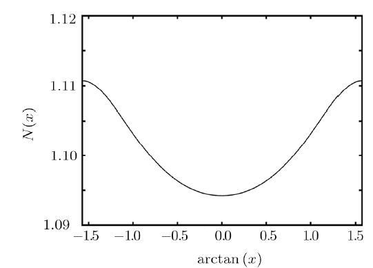
The energy is small for band center anomaly, so that the expansion can be used to obtain a solution for the stationary distribution. It is not well understood of $\rho(\theta)$ given by Eq. (16) for band center anomaly in weakly disordered chain. In Fig. 1, we plot numerical value of the normalization factor $N(x)$ for the invariant distribution. It shows $N(x)$ is of order $1$. We included a scaling factor in $\rho(\theta)$ and scaled $N(x)$ to order $1$ from $x \to 0$ to $x \to \infty$, but it is hard to see in Fig. 1 what kind of function of $x$ it is. Without a simple analytical expression for $N(x)$, one cannot give a full $x$ range description for $\gamma(x)$. At the end of this section, we will give a Padé approximation for $\gamma(x)$ for any magnitude of $x$.Fig. 1
 New window|Download| PPT slide
Fig. 1The normalization factor $ N(x)$. The full line is the normalization factor in Eq. (16), $x=E/\sigma^2$, and the horizontal axis in $\arctan(x)$ is used to show all possible magnitude of $x$.
Let us return to the differential equation. The ratio $x$ is free to choose and that is the primary dilemma we encounter. Considering $x\ll 1$, if we neglect the terms with respect to $x$, the differential equation Eq. (15) becomes
with the normalized solution for distribution[13]
When $x$ approaches infinity, Eq. (15) reduces to
which means $\rho(\theta)$ is a constant, $\rho(\theta)={1}/{\pi}$.
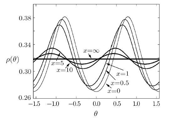
In Fig. 2, we plot the invariant distribution function $\rho(\theta)$ according to Eq. (16). It demonstrates that, as $x\rightarrow 0$, the distributions collapse on Eq. (24). As $x$ getting close to infinity, the distribution function gradually becomes flat and the amplitude of oscillation is decreasing. These properties of the solution for general $x$ are in agreement with above analysis for the limiting cases discussed.
Fig. 2
 New window|Download| PPT slide
Fig. 2Invariant distribution $\rho(\theta)$ for $x=0$, $0.5$, $1$,$5$, $10$, and $\infty$, respectively. The lines with oscillation amplitudes from big to small are in correspondence with the magnitude of $x$ from small to big, one by one. The flat $\rho(\theta)$ line is of $E/\sigma^2=\infty$.
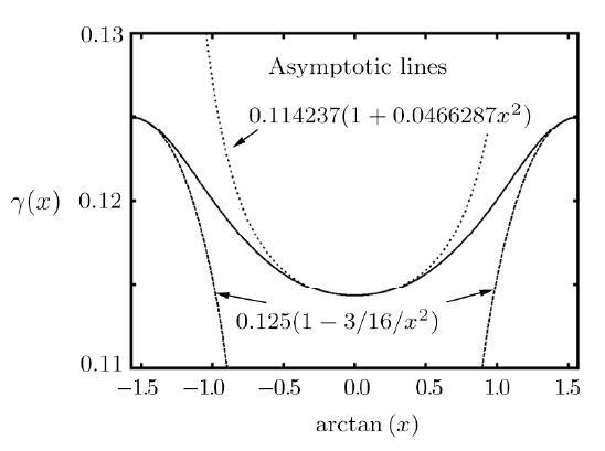
In Fig. 3 we plot the numerical values of Lyapunov exponent $\gamma(x)$ in Eq. (17) for all possible $x$. We plot in the same figure also the asymptotic behaviors of Lyapunov exponent for $x\to 0$ and $x\to\infty$ according to Eqs. (20) and (22). As shown in Fig. 3, the leading correction terms in the asymptotic series can give a good description for a certain range when $x$ is big or small. An expression for $\gamma(x)$ for the middle magnitude $x$ should be interesting.
Fig. 3
 New window|Download| PPT slide
Fig. 3Lyapunov exponent $\gamma(x)$ in unit of $\sigma^2$. The full line is the Lyapunov exponent in Eq. (17). The dashed and dotted lines are the asymptotic behavior upto the first correction term for $x\to\infty$ and $x\to 0$, respectively.
In Ref. [17], such an expression has been obtained by fitting numerically obtained $\gamma(x)$ in that work,
$$ \gamma(x)=\gamma_p\Big[1-\frac{0.086}{1+(x/1.426)^2}+\cdots\Big]\,, $$
where $\gamma_p = {\sigma^2}/{8(1-E^2/4)}$ is the perturbation result first obtained by Thouless.[12] In Fig. 3 we will not be able to resolve the difference between the full line and this fitting curve if we plot them together. This fitting matches the small $x$ region well and the coefficient of $x^2$ correction term has two accurate digits. However, the asymptotic behavior in $x\to \infty$ is wrong.
At the end of this section, we give a Padé approximation for $\gamma(x)$ for any magnitude of $x$ for practical use. For describing the whole anomalous region in the vicinity of band center, one can write down a rational Padé approximation without free parameters,
Since $\gamma(0)$ and $\gamma(\infty)$ have been already found, the $-3/16$ and 0.046 628 7 coefficients in leading correction terms in Eq. (20) and Eq. (22) completely fixed the coefficients of $x^2$ terms in this Padé approximation.
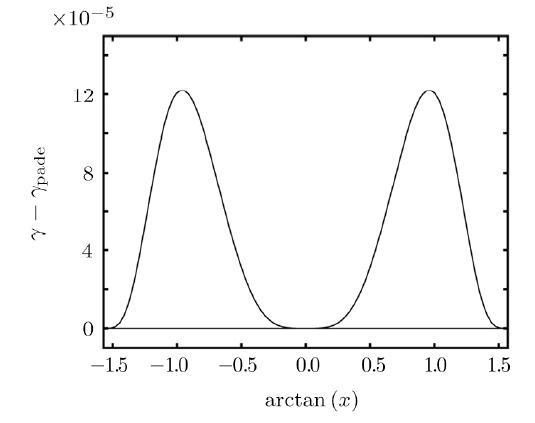
In Fig. 4, the difference between $\gamma(x)$ and the Padé approximation formula is plotted. It shows that the approximation is very good when $x$ is big or small. The maximum difference is of order $1\times 10^{-4}$, which appears at a middle magnitude $x$. $\gamma(x)/\sigma^2$ has been shown to be of order $0.1$ in Fig. 3. Now we have an approximated expression with at least four accurate digits for $\gamma(x)$.
Fig. 4
 New window|Download| PPT slide
Fig. 4The difference between the numerical values of Lyapunov exponent $\gamma(x)$ in Eq. (17) and its Padé approximation $\gamma_{\rm pade}(x)$ in Eq. (26). The full line is the difference in unit of $\sigma^2$.
In conclusion, we analytically studied the properties of the Lyapunov expoent in the vicinity of $E=0$ for one-dimensional Anderson model with diagonal random potential. By implementing the parametrization method, we obtained the recursion integration equation for invariant distribution function. In the weak disorder and band center case, a differential equation involving the ratio of energy and disorder strength $x=E/\sigma^2$ is derived. The solution of this equation is given to show that this ratio $x$ directly affects the invariant distribution as well as the behavior of Lyapunov exponent. Finally, we presented a Padé approximation formula which could not only reproduce the Thouless formula and anomaly within their valid range respectively, but also provide a transparent way to describe the transition. As it was pointed out in Ref. [17], higher order terms in $x$ exist, a simple analytical function of $x$ is still to be found for Lyapunov exponent.
Acknowledgments
The authors thank Profs. Zhou Sen, Xu Yuan-Yuan, Wu Long-Biao, Zhou Hao, Huang Yun-Peng for discussions.Reference By original order
By published year
By cited within times
By Impact factor
DOI:10.1103/PhysRev.109.1492URL [Cited within: 1]
DOI:10.1103/PhysRevLett.84.2913URL [Cited within: 1]
DOI:10.1103/PhysRevLett.91.096601URLPMID:14525198

We resolve the problem of the violation of single parameter scaling at the zero energy of the Anderson tight-binding model with diagonal disorder. It follows from the symmetry properties of the tight-binding Hamiltonian that this spectral point is, in fact, a boundary between two adjacent bands. The states in the vicinity of this energy behave similarly to states at other band boundaries, which are known to violate single parameter scaling.
DOI:10.1016/j.physleta.2003.11.033URL
We study some mesoscopic properties of electron transport by employing one-dimensional chains and Anderson tight-binding model. Principal attention is paid to the resistance of finite-length chains with disordered white-noise potential. We develop a new version of the transfer matrix approach based on the equivalency of a discrete Schr dinger equation and a two-dimensional Hamiltonian map describing a parametric kicked oscillator. In the two limiting cases of ballistic and localized regime we demonstrate how analytical results for the mean resistance and its second moment can be derived directly from the averaging over classical trajectories of the Hamiltonian map. We also discuss the implication of the single parameter scaling hypothesis to the resistance.
DOI:10.1103/PhysRevB.24.5698URL
We examine the nature of the zero-energy state in a one-dimensional tight-binding system with only nearest-neighbor off-diagonal disorder. We find that, although the localization length diverges at this energy, the state must nevertheless be considered as localized because the mean values of the transmission coefficient (which is directly related with the dc conductance) approach zero as the size of the system L goes to infinity. In particular, we find that the geometric and harmonic mean values of the transmission coefficient behave as exp(-γL), while the arithmetic mean value follows the power law Lwith δ~=0.50. This is in contrast with the usual case of only diagonal disorder, where all three means behave as exp(-λL).
DOI:10.1103/PhysRevLett.95.020401URL [Cited within: 1]
DOI:10.1007/BF01295469URL [Cited within: 1]
The localization of the electron states and dc-conductivity of the one dimensional Anderson model are investigated with various numerical procedures. It is found that the eigenstates are always exponentially localized and that in the center of the band the localization length is proportional to the inverse square of the disorder. The dc-conductivity, as obtained by using the Kubo-Greenwood formula, obeys the central limit theorem for any finite imaginary frequency, with a variance, which is inversely proportional to the squareroot of the number of states contributing to the transport. There is no exponential length dependence of the Kubo-Greenwood conductivity within this model. The conductivity tends to zero only in the limit of vanishing imaginary frequency.
DOI:10.1088/0022-3719/19/22/015URL [Cited within: 1]
The author presents a numerical method for calculating the integrated density of states and the localisation length in quasi-one-dimensional tight-binding disordered systems. The results for the one-dimensional Anderson model with off-diagonal disorder confirm that the singularities for the density of states and the localisation length are in the form predicted by Dyson. In two dimensions the singularity for the density of states near E=0 approaches the form rho (E) varies as E- phi for weak off-diagonal disorder. The author obtained approximately 1/3 for the exponent phi consistent with current fractal viewpoints. Some results for strong off-diagonal disorder in two dimensions where the singularity is of a different nature are also presented.
DOI:10.1007/BF01312150URL [Cited within: 1]
We study the E -dependence of the Lyapounov exponent of an electron with energy E in the one dimensional Anderson model with off diagonal disorder. In the neighbourhood of the band centre we find for nonzero disorder 65log 611 E →0 for E →0, but all even moments of Reγ( E ) diverge logarithmically. As the probability of Re γ( E )=0 decreases to zero for E →0 we conclude that the electron is always exponentially localised.
DOI:10.1103/PhysRevB.89.075434URL [Cited within: 1]
In this paper, we explore the localization transition and the scaling properties of both quasi-one-dimensional and two-dimensional quasiperiodic systems, which are constituted from coupling several Aubry-Andre (AA) chains along the transverse direction, in the presence of next-nearest-neighbor (NNN) hopping. The localization length, two-terminal conductance, and participation ratio are calculated within the tight-binding Hamiltonian. Our results reveal that a metal-insulator transition could be driven in these systems not only by changing the NNN hopping integral but also by the dimensionality effects. These results are general and hold by coupling distinct AA chains with various model parameters. Furthermore, we show from finite-size scaling that the transport properties of the two-dimensional quasiperiodic system can be described by a single parameter and the scaling function can reach the value 1, contrary to the scaling theory of localization of disordered systems. The underlying physical mechanism is discussed.
DOI:10.1007/BF01294272URL [Cited within: 1]
We calculate the density of states and various characteristic lengths of the one-dimensional Anderson model in the limit of weak disorder. All these quantities show anomalous fluctuations near the band centre. This has already been observed for the density of states in a different model by Gorkov and Dorokhov, and is in close agreement with a Monte-Carlo calculation for the localization length by Czycholl, Kramer and Mac-Kinnon.
[Cited within: 2]
DOI:10.1103/PhysRevB.49.14504URLPMID:10010535 [Cited within: 4]
A uniform quantitative description of the properties of the one-dimensional Anderson model is obtained by mapping that problem onto an infinitely quasidegenerate master equation. This quasidegeneracy is identified as the source of the small-denominator problem encountered before in investigations of this problem. An appropriate quasidegenerate perturbation theory is developed to obtain a uniform asymptotic expansion, in powers of the strength of the noise, for the probability distribution function of the ratio of the value of the wave function at neighboring sites. Well known results, such as those obtained by Thouless, Kappus and Wegner, and Derrida and co-workers are reproduced and systematic corrections to these results as well as some more results are found. In particular, we find internal layers in the above-mentioned distribution function for values of the energy given by E=2 cos\ensuremath{\pi}\ensuremath{\alpha} with \ensuremath{\alpha} rational. We also find crossovers in the behavior of the distribution function (and consequently in quantities derived from it) near the band-edge and band-center regions. The properties of the model in the band-edge region were studied by us in detail in a previous publication [Phys. Rev. B 47, 1918 (1992)].
DOI:10.1051/jphys:019840045080128300URL [Cited within: 1]
DOI:10.1103/PhysRevB.25.4304URL [Cited within: 1]
A transfer operator method is used to calculate the inverse localization length, α, of the one-dimensional Anderson model as a function of disorder, σ. For small disorder α vanishes as α=Aσ+O(σ), with A=0.2088.
DOI:10.1007/BF01028469URL [Cited within: 1]
We show that the formal perturbation expansion of the invariant measure for the Anderson model in one dimension has singularities at all energies E 0 =2 cos π ( p/q ); we derive a modified expansion near these energies that we show to have finite coefficients to all orders. Moreover, we show that the first q 613 of them coincide with those of the “naive” expansion, while there is an anomaly in the ( q 612)th term. This also gives a weak disorder expansion for the Liapunov exponent and for the density of states. This generalizes previous results of Kappus and Wegner and of Derrida and Gardner.
DOI:10.1016/j.physleta.2011.08.015URL [Cited within: 3]
78 We study the band center anomaly of one-dimensional Anderson localization. 78 We study numerically the Lyapunov exponent through a parametrization method of the transfer matrix. 78 We give a unified equation to describe the band center anomaly and perturbation theory.
DOI:10.1088/0253-6102/54/4/28URL [Cited within: 3]
DOI:10.1016/j.physe.2017.12.010URL [Cited within: 2]
We consider the one-dimensional Anderson model with weak disorder. Using the Hamiltonian map approach, we analyse the validity of the random-phase approximation for resonant values of the energy, E = 2 cos( r) , with r a rational number. We expand the invariant measure of the phase variable in powers of the disorder strength and we show that, contrary to what happens at the centre and at the edges of the band, for all other resonant energies the leading term of the invariant measure is uniform. When higher-order terms are taken into account, a modulation of the invariant measure appears for all resonant values of the energy. This implies that, when the localisation length is computed within the second-order approximation in the disorder strength, the Thouless formula is valid everywhere except at the band centre and at the band edges.
DOI:10.1088/0305-4470/31/23/008URL [Cited within: 1]
A new approach is applied to the one-dimensional Anderson model by using a two-dimensional Hamiltonian map. For a weak disorder this approach allows for a simple derivation of correct expressions for the localization length both at the centre and at the edge of the energy band, where standard perturbation theory fails. Approximate analytical expressions for strong disorder are also obtained.
DOI:10.1016/j.physe.2012.01.024URL [Cited within: 5]
78 Focus: the band-centre anomaly in the 1D Anderson model with diagonal disorder. 78 Result: analytical expression of the localisation length close to the band centre. 78 Remark: extension of the Derrida–Gardner formula beyond the exact band centre. 78 Discussion: implications for the validity of the single-parameter scaling hypothesis.
