Saeed Ullah Jan², Sami Ul Haq², Syed Inayat Ali Shah², Ilyas Khan^,1,*?, Muhammad Atif Khan³ 1 Faculty of Mathematics and Statistics,Ton Duc Thang University, Ho Chi Minh City, Vietnam;
2 Department of Mathematics, Islamia College University,Peshawar 25000, Pakistan;
3 Department of Mathematics, Kohat University of Science & Technology, Kohat 26000, Pakistan;

Corresponding authors: ? * E-mail:ilyaskhan@tdt.edu.vn

Received:2018-09-2Online:2019-06-1



PDF (2557KB)MetadataMetricsRelated articlesExportEndNote|Ris|BibtexFavorite
Cite this article
Saeed Ullah Jan, Sami Ul Haq, Syed Inayat Ali Shah, Ilyas Khan, Muhammad Atif Khan. General Solution for Unsteady Natural Convection Flow with Heat and Mass in the Presence of Wall Slip and Ramped Wall Temperature. [J], 2019, 71(6): 647-657 doi:10.1088/0253-6102/71/6/647

Nomenclature

1 Introduction

In the literature, the theoretical study of laminar free convection flow from a vertical plate is continuously receiving the attention of researchers due to their technological and industrial applications. In fluid mechanics, the solutions of the non-dimensional governing equations have been attempted by analytical and numerical techniques. A number of unsteady natural convection flows past a vertical plate covered by various set of thermal conditions at the bounding plate have been investigated.^[1-3] Many applied problems may be demanded by considering wall conditions, which are arbitrary or non-uniform. Hayday et al.^[4] added the numerical solutions for non-similar boundary layer laminar flows over a vertical plate under the effect of temperature. Fully expanded laminar flows are examined by Schetz.^[5] He obtained the approximate and analytical solutions for such two dimensional flow under thermal effects. Later on, the analytical work to refine earlier solutions for the variation of various types of wall temperature was tried by Kao,^[6] Kelleher,^[7] and Yovanovich.^[8] Soundalgekar^[9] and Ingham^[10] firstly found the exact solution for the incompressible viscous fluid near vertical plates for the natural convection flow. The work of Soundalgekar^[9] and Ingham^[10] over the convectional flows was further extended by Singh and Kumar,^[11] Soundalgekar and Gupta^[12] and Raptis et al.^[13] Magnetic effects on the flow of viscous fluid were also studied by Raptis and Singh.^[13] These solutions provided a new streamline for the researchers to investigate different heat flow problems under the influence of magnetic field. Solution for the oscillating flow of viscous fluid with slip boundary condition is established by Khaled and Vafai.^[14] Buoyancy forces that are the results of density distinction are responsible for the free convection flow of fluid. Many researchers used free convection flow due to enormous applications in industrial and natural sciences, such as liquid crystals, cooling of electron components, chemical suspensions, and dilute suspensions.^[15]

In mechanics of fluids we can use two types of boundary conditions in different flow problems i.e. slip and no slip boundary conditions If there is no corresponding motion between the fluid and wall directly in connection with the wall, then it would be no-slip boundary condition. Maybe for the simplification of difficult situation, this condition is used extensively but it has also some impediment. There are few sufficiently smooth surfaces where the wall and fluid have no connections and the fluid slips against the wall.^[16] For example, the no-slip condition is not able to work in the capillaries.^[17] However, these impediments which are mentioned by the Navier in his beginning work,^[18] are overcome by the slip condition. Slip condition is also called Navier condition. The slip condition has various applications in different fields of medical science, extrusion, lubrication, particularly in flows through porous media, polishing artificial heart valves, micro and Nano fluids, studies of friction at different surfaces and biological fluids.^[19-20] In the last few years, many authors used the slip condition for the flows of viscous fluids.^[21-23]

Natural convection flow of a fluid which is electrically conducting and flowing at a vertically moving plate having ramped temperature, is examined by Ghara et al.^[24] Seth et al.^[25] discussed the impulsive plate driven flows and examined the Soret as well as Hall effects over such MHD flows, where the suction phenomenon in such flows through a porous plate is considered by Reddy.^[26] Samiulhaq et al.^[27] investigated a second-grade fluid for Magneto hydrodynamic natural convection flow. The unsteady MHD natural convection flows near an accelerated vertical plate along temperature source and constant heat flux was investigated by Narahari and Debnath.^[28] Micropolar fluid with slip condition and periodic temperature passed through a porous medium in Magneto hydrodynamic natural convection flow was studied by Mansour et al.^[29]

The purpose of present work is the investigation of the impact of slip wall conditions on unsteady natural convection flows with the phenomena of heat transfer and the ramped wall temperature. We consider the slippage as well as ramped wall temperature, at the boundary. Analytical solutions of the non-dimensional governing equation i.e. temperature, concentration and velocity are obtained by integral transform method (Laplace transform). Numerical tables for Skin-friction, Sherwood number and Nusselt-number are examined. At the end, graphical explanation for velocity, temperature, concentration, Skin-friction, Sherwood number and Nusselt-number are presented and the impacts of involved physical parameters are observed.

2 Analysis of the Governing Problem

Let us consider the unsteady flow of incompressible viscous fluid with the influence of slippage over the boundary. The pressure variations are assumed to be negligible. Motion of the fluid is induced subject to slippage of fluid at the surface of the plate. The plate is considered along $x'$-axis in the upward direction and $y'$-axis is perpendicular to the plate. At the initial stage for $t'\leq 0$, both the fluid and the plate is assumed to be stationary at the same temperature $T^{\prime}_{\infty}$ and concentration $C^{\prime}_{\infty}$. When $0 <t'\leq t_{0}$ the temperature of the plate is elevated or declined to $T^{\prime}_{\infty}+(T_{w}^{\prime}-T_{\infty}')({t'}/{t_{0}})$ and on the other hand for $t'> t_{0}$ the temperature of the plate is kept at uniform temperature $T^{\prime}_{w}$ and the level concentration of the fluid at plate is elevated to $C_{w}'$ or concentrations is accumulated to the plate at constant rate. By Boussinesq's approximation the unsteady incompressible viscous fluid, which flows near infinite vertical plate is investigated by.^[30-32]

(1) $\frac{\partial{u^{\prime}}}{\partial{t^{\prime}}}={g}\beta(T^{\prime}-T_{\infty}') +g\beta^{\ast}(C^{\prime}-C_{\infty}')+\nu\frac{\partial^2 {u'}}{\partial {y^{\prime 2}}}\,,$
(2) $\rho C_{p}\frac{\partial{T^{\prime}}}{\partial{t'}}= k\frac{\partial^2 {T^{\prime}}}{\partial {y^{\prime 2}}}\,,$
(3) $\frac{\partial{C'}}{\partial{t'}}={D}\frac{\partial^2 {C'}}{\partial {y^{\prime 2}}}\,.$
The corresponding initial and boundary conditions were under as:

(4) $u^{\prime}=0\,,\quad {T^{\prime}=T^{\prime}_{\infty}}\,,\quad {C'=C^{\prime}_{\infty}}\quad \text{for}\quad t'=0\,,\quad y^{\prime}\geq 0\,, \\ u^{\prime}=\lambda\frac{\partial {u'}}{\partial y^{\prime}}\quad \text{for}\quad t'>0\,, \quad y^{\prime}=0\,, \\ T'=\left\{\begin{matrix} T^{\prime}_{\infty}+(T^{\prime}_{w}-T^{\prime}_{\infty})\displaystyle\frac{t^{\prime}}{t_{0}}\quad \text{for}\quad 0<t^{\prime}\leq t_{0}\,, \\ T^{\prime}_{w}\quad \text{for}\quad t^{\prime}>t_{0}\, \\ \end{matrix}\right. \\ C^{\prime}={C^{\prime}_{w}} \quad \text{for}\quad t'>0\,, \\ u^{\prime}\rightarrow 0,\quad T^{\prime}\rightarrow T^{\prime}_{\infty},\quad C^{\prime}\rightarrow C^{\prime}_{\infty} \quad \text{as} \quad y^{\prime}\rightarrow \infty\,,$
where $\lambda$ is the dimensional slip parameter. The imposed condition on the velocity is identical to those obtained by Samiulhaq et al.^[33] while on the temperature and concentration is identical to those obtained by Narahari et al.^[34] and Nehad et al.^[35] To convert the governing equation into non-dimensional form, we introduce a set of non-dimensional variables

(5) $\zeta=\frac{y^{\prime}}{\sqrt{\nu t_{0}}}\,,\quad\tau=\frac{t^{\prime}}{t_{0}}\,,\quad {\upsilon}=\frac{u^{\prime}}{t_{0}g\beta(T^{\prime}_{w}-T^{\prime}_{\infty})}\,, \\ \text{or}\quad{\upsilon}=\frac{u^{\prime}}{Gr}\sqrt{\frac{t_{0}}{\nu}}\,, \quad{\Theta}=\frac{(T^{\prime}-T^{\prime}_{\infty})}{(T^{\prime}_{w}-T^{\prime}_{\infty})}\,, \\ Pr =\frac{\mu C_{p}}{k}\,,\quad {Gr}=\frac{g\beta(T^{\prime}_{w}-T^{\prime}_{\infty}) t^{{3}/{2}}_{0}}{\sqrt{\nu}}\,, \\ {\Psi}=\frac{C^{\prime}-C^{\prime}_{\infty}}{C^{\prime}_{w}-C^{\prime}_{\infty}}\,, \quad \text{or} \quad{\Psi}=\frac{C^{\prime}-C^{\prime}_{\infty}}{({j^{\prime\prime}\sqrt{\nu t_{0}}}/{D})}\,, \\ {Sc}=\frac{\nu}{D}\,,\quad {\eta}=\frac{\lambda}{\sqrt{\nu t_{0}}}\,, \quad {Gm}=\frac{g\beta^{*}(C^{\prime}_{w}-C^{\prime}_{\infty})t^{{3}/{2}}_{0}}{\sqrt{\nu}}\,, \\ \text{or} \quad{Gm}=\frac{g\beta^{*}j^{\prime\prime} t^{2}_{0}}{D}\,,\quad N=\frac{Gm}{Gr}\,.$
As the flow is fully developed over a plate of infinite length, so the physical variables are functions of $y^{\prime}$ and $t^{\prime}$, where $u^{\prime}$ denotes the dimensional velocity in $x'$-direction. Using these non-dimensional variables (5) in Eqs. (1), (2), and (3), the governing equations (1), (2), and (3) take the simplest forms

(6) $\frac{\partial{\upsilon(\zeta,\tau)}}{\partial{\tau}} =\Theta(\zeta,\tau)+{N}{\Psi(\zeta,\tau)}+\frac{\partial^{2} \upsilon(\zeta,\tau)}{\partial \zeta^{2}}\,,$
(7) $Pr\frac{\partial{\Theta(\zeta,\tau)}}{\partial{\tau}} =\frac{\partial^{2} \Theta(\zeta,\tau)}{\partial \zeta^{2}}\,,$
(8) $Sc\frac{\partial{\Psi(\zeta,\tau)}}{\partial{\tau}} =\frac{\partial^{2} \Psi(\zeta,\tau)}{\partial \zeta^{2}}\,,$
where $\upsilon$ denotes the velocity in non-dimensional form, $\zeta$ is coordinate axis which is normal to the plates in non-dimensional form, $\tau$ is time in non-dimensional form, $\Theta$ is temperature in non-dimensional form, $\Psi$ is concentration in non-dimensional form, $Gm$ is mass Grashof number, $Gr$ is thermal Grashof number, $Sc$ is Schmidt number, $Pr$ is Prandtl number, $N$ is the mass to thermal buoyancy ratio parameter. Moreover, characteristics time $t_{0}$ can be defined as

(9) $t_{0}=\Bigl[\frac{\nu}{g^{2}\beta^{2}(T^{\prime}_{w}-T^{\prime}_{\infty})^{2}}\Bigr]^{{1}/{3}}
is identical to that of Samiulhaq et al.^[33] and Narahari et al.^[36] Corresponding initial and boundary condition (4) in the non-dimensional form which are:

(10) $\upsilon(\zeta,0)=0\,,\quad \Theta(\zeta,0)=0\,, \quad \Psi(\zeta,0)=0,\quad for \quad \zeta\geq 0 \,, \\ \upsilon(0,\tau)=\eta\frac{\partial{\upsilon(0,\tau)}} {\partial{\zeta}}\,, \quad for \quad \tau > 0\,, \\ \Theta(0,\tau)= \tau \quad for \quad \tau\leq1\,, \\ 1 \quad for \quad \tau >1 \quad for \quad \tau >0\,, \\ \Psi(0,\tau)=1\,, \quad for \quad \tau >0\,, \\ \upsilon(\zeta,\tau)\rightarrow 0\,,\quad \Theta(\zeta,\tau)\rightarrow 0\,, \quad \Psi(\zeta,\tau)\rightarrow 0\,, \\ as \quad \zeta\rightarrow\infty \quad for \quad \tau > 0\,,$
where $\eta$ is the dimensionless slip parameter.

3 Analytical Laplace Transform Solutions

3.1 Solution of Ramped Temperature

Applying Laplace transforms to Eqs. (6), (7), (8) and using initial and boundary condition (10), we obtain the following problem for temperature, concentration and velocity for $Pr\neq1$, $Sc\neq1$, and $Pr=1$, $Sc=1$.

(i)Case 1 $Pr\neq1$, $Sc\neq1$,

(11) $\Theta(\zeta_{1},s)=(1-\text{exp}(-s))E(\zeta_{1},s)\,,$
(12) $\Psi(\zeta_{2},s)=E_{0}(\zeta_{2},s)\,,$
(13) $\upsilon(\zeta,s)\!=\!\frac{(1\!-\!\text{exp}(-s))}{Pr-1}[bE_{1}(\zeta,s) +\sqrt{Pr}E_{3}(\zeta,s)-E_{2}(\zeta_{1},s)] \\ +\frac{N}{Sc-1}[bE_{6}(\zeta,s)+\sqrt{Sc}E_{5}(\zeta,s) -E(\zeta_{2},s)],$
where

$ \zeta_{1}=\zeta\sqrt{Pr},\quad \zeta_{2}= \zeta\sqrt{Sc},\quad b= \frac{1}{\eta}\,, \\ E(\zeta_{1},s)= \frac{\exp(-\zeta_{1}\sqrt{s})}{s^{2}}, \quad \quad E(\zeta_{2},s)= \frac{\exp(-\zeta_{2}\sqrt{s})}{s^{2}}\,, \\ E_{0}(\zeta_{2},s)= \frac{\exp(-\zeta_{2}\sqrt{s})}{s},\quad \quad E_{1}(\zeta,s)= \frac{\exp(-\zeta\sqrt{s})}{s^{3}(\sqrt{s}+b)}\,, \\ E_{2}(\zeta_{1},s)= \frac{\exp(-\zeta_{1}\sqrt{s})}{s^{3}}\,, \quad \quad E_{3}(\zeta,s)= \frac{\exp(-\zeta\sqrt{s})}{s^{{5}/{2}}(\sqrt{s}+b)}\,, \\ E_{5}(\zeta,s)= \frac{\exp(-\zeta\sqrt{s})}{s^{{3}/{2}}(\sqrt{s}+b)}\,,\quad \quad E_{6}(\zeta,s)= \frac{\exp(-\zeta\sqrt{s})}{s^{2}(\sqrt{s}+b)}\,, \\ E(\zeta,s)=\frac{\exp(-\zeta\sqrt{s})}{s^{3}}\,. $

The inverse Laplace transform of Eqs. (11), (12), and (13) are

(14) $\Theta(\zeta_{1},\tau) =E(\zeta_{1},\tau)-E(\zeta_{1},\tau-1) H(\tau-1)\,,$
(15) $\Psi(\zeta_{2},\tau) =E_{0}(\zeta_{2},\tau)\,,$
(16) $\upsilon(\zeta,\tau) =\frac{1}{Pr-1}[bE_{1}(\zeta,\tau)+\sqrt{Pr}E_{3}(\zeta,\tau) -E_{2}(\zeta_{1},\tau) -\{bE_{1}(\zeta,\tau-1)+\sqrt{Pr}E_{3} (\zeta,\tau-1)-E_{2}(\zeta_{1},\tau-1)\}H(\tau-1)] \\ +\frac{N}{Sc-1}[bE_{6}(\zeta,\tau)+\sqrt{Sc}E_{5} (\zeta,\tau)-E(\zeta_{2},\tau)]\,,$
where

$ E(\zeta_{1},\tau)=\Bigl(\frac{Pr\zeta^{2}}{2}+\tau\Bigr) {\rm erfc}\Bigl(\frac{\zeta_{1}}{2\sqrt{\tau}}\Bigr) -\sqrt{\frac{Pr\tau}{\pi}}\zeta \exp\Bigl(\frac{Pr\zeta^{2}}{4\tau}\Bigr)\,,\quad E(\zeta_{2},\tau)=\Bigl(\frac{Sc\zeta^{2}}{2}+\tau\Bigr) {\rm erfc}\Bigl(\frac{\zeta_{2}}{2\sqrt{\tau}}\Bigr)-\sqrt{\frac{Sc\tau}{\pi}}\zeta \exp\Bigl(\frac{Sc\zeta^{2}}{4\tau}\Bigr)\,, \\ E_{0}(\zeta_{2},\tau)={\rm erfc}\Bigl(\frac{\zeta_{2}}{2\sqrt{\tau}}\Bigr)\,, \\ E_{1}(\zeta,\tau)=\tau^{2}\exp\Bigl(-\frac{b\zeta^{2}}{2}\Bigr)\sinh\Bigl(\frac{b\zeta}{2}\Bigr) +\frac{\tau^{2}}{2}\exp\Bigl(-\frac{b\zeta^{2}}{2}\Bigr)-\frac{b}{\pi} \int_{0}^{\tau}\int_{0}^{\infty}\Bigl(\frac{1-\exp(-xs)}{x^{2}}\Bigr) \Bigl[\frac{b\sin(\zeta\sqrt{x})}{x+b^{2}}+\frac{\sqrt{x} \cos(\zeta\sqrt{x})}{x+b^{2}}\Bigr]dxds\,, \\ E_{2}(\zeta_{1},\tau)=\frac{1}{2}\Bigl(\frac{Pr^{2}\zeta^{4}}{12}+Pr\zeta^{2}\tau+\tau^{2}\Bigr) {\rm erfc}\Bigl(\frac{\zeta_{1}}{2\sqrt{\tau}}\Bigr) -\sqrt{\frac{Pr \tau}{\pi}}\frac{\zeta}{6}\Bigl(\frac{Pr\zeta^{2}}{2}+5\tau\Bigr) \exp\Bigl(-\frac{Pr\zeta^{2}}{4\tau}\Bigr)\,, \\ E_{3}(\zeta,\tau)=\frac{1}{3b\sqrt{\pi}}\Bigl[\sqrt{\pi}\zeta^{3}+\sqrt{\tau}(4\tau-2\zeta^{2}) \exp\Bigl(-\frac{\zeta^{2}}{4\tau}\Bigr)-\sqrt{\pi}\zeta^{3}\Bigl(\frac{\zeta}{2\sqrt{\tau}}\Bigr)\Bigr] -\Bigl(\frac{1}{b^{2}}+\frac{\zeta}{b}\Bigr) \Bigl[\Bigl(\tau+\frac{\zeta^{2}}{2}\Bigr){\rm erfc}\Bigl(\frac{\zeta}{2\sqrt{\tau}}\Bigr)-\sqrt{\frac{\tau}{\pi}}\zeta \exp\Bigl(\frac{-\zeta^{2}}{4\tau}\Bigr)\Bigr] \\ +\frac{\exp(b\zeta)}{b^{2}}\int_{0}^{\tau} \exp(b^{2}s) {\rm erfc}\Bigl(\frac{\zeta+2bs}{2\sqrt{\tau}}\Bigr)d s\,, \\ E_{5}(\zeta,\tau)=\frac{2}{b}\Bigl[\sqrt{\frac{\pi}{t}}\exp\Bigl(\frac{-\zeta^{2}}{4\tau}\Bigr) -\Bigl(\frac{1}{b^{2}}+\frac{\zeta}{b}\Bigr){\rm erfc}\Bigl(\frac{\zeta}{2\sqrt{\tau}}\Bigr) +\frac{1}{b^{2}}\exp(b\zeta+b^{2}\tau) {\rm erfc}\Bigl(\frac{\zeta+2b\tau}{2\sqrt{\tau}}\Bigr)\Bigr]\,, \\ E_{6}(\zeta,\tau)=\frac{1}{\pi}\int_{0}^{\infty}\Bigl(\frac{\tau}{x} -\frac{1-\exp(-x\tau)}{x^{2}}\Bigr) \Bigl[\frac{b\sin(\zeta\sqrt{x})}{x+b^{2}} +\frac{\sqrt{x}\cos(\zeta\sqrt{x})}{x+b^{2}}\Bigr]d x\,. $

$H(\tau-1)$ is the unit step function defined as

(17) $H(\tau-c)= \cases 0 \quad \text{for} \quad 0\leq\tau<c\,,\\ 1 \quad \text{for} \quad\tau\geq c\,, $
where $c$ is an arbitrary constant.

(ii)Case 2$Pr=1$, $Sc=1$,

(18) $\Theta(\zeta,s)=(1-\exp(-s))E(\zeta,s)\,,$
(19) $\Psi(\zeta,s)=E_{0}(\zeta,s)\,,$
(20) $\upsilon(\zeta,s)=\frac{(1-\exp(-s))}{2}[E_{3} (\zeta,s)+\zeta E_{4}(\zeta,s)] \\ +\frac{N}{2}[E_{5}(\zeta,s)+E_{7}(\zeta,s)]\,,$
where

$ E(\zeta,s)=\frac{\exp(-\zeta\sqrt{s})}{s^{2}}\,, \quad E_{0}(\zeta,s)=\frac{\exp(-\zeta\sqrt{s})}{s}\,, \\ E_{4}(\zeta,s)= \frac{\exp(-\zeta\sqrt{s})}{s^{{5}/{2}}}\,, \quad E_{7}(\zeta,s)= \frac{\exp(-\zeta\sqrt{s})}{s^{{3}/{2}}}\,. $

The inverse Laplace transform of Eqs. (18), (19), and (20) are

(21) $\Theta(\zeta,\tau)=E(\zeta,\tau)-E(\zeta,\tau-1)H(\tau-1)\,,$
(22) $\Psi(\zeta,\tau)=E_{0}(\zeta,\tau)\,,$
(23) $\upsilon(\zeta,\tau)=\frac{1}{2}[E_{3}(\zeta,\tau)+\zeta E_{4}(\zeta,\tau)-\{E_{3}(\zeta,\tau-1) \\ +\zeta E_{4}(\zeta,\tau-1)\}H(\tau-1)] \\ +\frac{N}{2}[E_{5}(\zeta,\tau)+\zeta E_{7}(\zeta,\tau)]\,,$
where

$E_{4}(\zeta,\tau)=\sqrt{\frac{\tau}{\pi}}\frac{\zeta}{3} (\zeta^{2}+4\tau)\exp\Bigl(\frac{-\zeta^{2}}{4\tau}\Bigr) \\ -\zeta^{2}\Bigl(\frac{\zeta^{2}}{6}+\tau\Bigr){\rm erfc}\Bigl(\frac{\zeta} {2\sqrt{\tau}}\Bigr)\,, \\ E_{7}(\zeta,\tau)=2\sqrt{\frac{\tau}{\pi}}-\zeta {\rm erfc}\Bigl(\frac{\zeta}{2\sqrt{\tau}}\Bigr)\,. $

(iii)Nusselt Number The corresponding Nusselt number in case of ramped temperature, which is the measure of the rate of heat transfer at the plate can be determined by differentiating Eq. (14) partially with respect to $"\zeta"$

${Nu(\tau)}=-\frac{\partial{\Theta(\zeta_{1},\tau)}}{\partial{\zeta}}\,,\quad \tau > 0\,,$

using $\zeta=0$, we get

(24)${Nu(\tau)}=2\sqrt{\frac{Pr}{\pi}}[\sqrt{\tau}-\sqrt{\tau-1}H(t-1)]\,.$
Also the corresponding Nusselt number can be determined by differentiating Eq. (21) partially with respect to $"\zeta"$ and using $\zeta=0$, we get

(25)${Nu(\tau)}=\frac{2}{\sqrt{\pi}}[\sqrt{\tau}-\sqrt{\tau-1}H(t-1)]\,.$
(iv)Sherwood Number The corresponding Sherwood number in case of ramped temperature which the measure of the ratio of convective and diffusive mass transfer can be determined by differentiating Eq. (15) partially with respect to $"\zeta"$

${Sh(\tau)}=-\frac{\partial{\Psi(\zeta_{2},\tau)}}{\partial{\zeta}}\,, \quad \tau>0\,,$

using $\zeta=0$, we get

(26)${Sh(\tau)}=\sqrt{{Sc}/({\pi\tau})}\,.$
Also the corresponding Sherwood number can be determined by differentiating Eq. (22) partially with respect to $"\zeta"$ and using $\zeta=0$, we get

(27)${Sh(\tau)}={1}/{\sqrt{\pi\tau}}\,.$
(v)Skin-frictionThe corresponding Skin-friction in case of ramped

temperature, which is the measure of the rate of shear stress at the

plate can be determined by differentiating Eq. (16) partially with

respect to $"\zeta"$

${C_{f}(\tau)}=-\frac{\partial{\upsilon(\zeta,\tau)}}{\partial{\zeta}}\,, \quad \tau>0\,,$

using $\zeta=0 $, we get

(28) ${C_{f}(\tau)}=\frac{1}{Pr-1}[bB_{1}(\tau)+\sqrt{Pr}B_{3}(\tau)-B_{2}(\tau) \\ -\{bB_{1}(\tau-1)+\sqrt{Pr}B_{3}(\tau-1) \\ -B_{2}(\tau-1)\}H(\tau-1)]+\frac{N}{Sc-1}[bB_{6}(\tau) \\ +\sqrt{Sc}B_{5}(\tau)-V(\tau)]\,,$
where

$ B_{1}(\tau)=\frac{b\tau^{2}}{2}-\Bigl[\frac{\exp(b^{2}\tau)}{b^{3}}{\rm erfc}(b\sqrt{\tau}) -\frac{1}{b^{3}}-\frac{\tau}{b} \\ +\frac{4\tau^{{3}/{2}}}{3\sqrt{\pi}} +\frac{2}{b^{2}}\sqrt{\frac{\tau}{\pi}}\Bigr]\,, \\ B_{2}(\tau)= -\frac{4}{3}\sqrt{\frac{Pr}{\pi}}\tau^{{3}/{2}}\,, \\ B_{3}(\tau)=\frac{\sqrt{Pr}}{b^{3}}\Bigl[\exp(b^{2}\tau){\rm erfc}(b\sqrt{\tau}) +2b\sqrt{\frac{\tau}{\pi}}-b^{2}\tau-1\Bigr]\,, \\ B_{5}(\tau)=\frac{2}{b^{2}}[\exp(b^{2}\tau){\rm erfc}(b\sqrt{\tau})-1]\,, \\ B_{6}(\tau)=\tau+\Bigl[\frac{1}{b^{2}}-\frac{2}{b}\sqrt{\frac{\tau}{\pi}} -\frac{\exp(b^{2}\tau)}{b^{2}}{\rm erfc}(b\sqrt{\tau})\Bigr]\,, \\ V(\tau)= -2\sqrt{\frac{Sc\tau}{\pi}}\,. $

Also, corresponding Skin-friction can be determined by differentiating Eq. (23) partially with respect to $"\zeta"$ and using $\zeta=0$, we get

(29)$C_{f}(\tau) = \frac{1}{2}[B_{3}(\tau)-B_{3}(\tau-1)H(\tau-1)] \\ +\frac{N}{2}[B_{5}(\tau)+E_{7}(\tau)]\,.$

3.2 Solution of Stepped Temperature

To investigate the ramped temperature effect of the fluid flow on the boundary, it is essential to compare the flows with the one nearby the isothermal plate. Under this assumption, it can be displayed that the non-dimensional temperature, concentration, and velocity variable can be expressed by applying Laplace transforms to Eqs. (6), (7) and (8) and using initial and boundary condition (10).

(i) Case 1 $Pr\neq 1$, $Sc\neq 1$,

(30) $\Theta(\zeta_{1},s)=E_{0}(\zeta_{1},s)\,,$
(31) $\Psi(\zeta_{2},s)=E_{0}(\zeta_{2},s)\,,$
(32) $\upsilon(\zeta,s)=\frac{1}{Pr-1}[bE_{6}(\zeta,s)+\sqrt{Pr}E_{5}(\zeta,s)-E(\zeta_{1},s)] \\ +\frac{N}{Sc-1}[bE_{6}(\zeta,s)+\sqrt{Sc}E_{5}(\zeta,s)-E(\zeta_{2},s)]\,,$
where

$E(\zeta_{1},s)= \frac{\exp(-\zeta_{1}\sqrt{s})}{s^{2}}\,, \quad E(\zeta_{2},s)= \frac{\exp(-\zeta_{2}\sqrt{s})}{s^{2}}, \\ E_{0}(\zeta_{1},s)= \frac{\exp(-\zeta_{1}\sqrt{s})}{s}\,, \quad E_{0}(\zeta_{2},s)= \frac{\exp(-\zeta_{2}\sqrt{s})}{s}\,. $

The inverse Laplace transform of Eqs. (30), (31), and (32) are

(33) $\Theta(\zeta_{1},\tau)=E_{0}(\zeta_{1},\tau)\,,$
(34) $\Psi(\zeta_{2},\tau)=E_{0}(\zeta_{2},\tau)\,,$
(35) $\upsilon(\zeta,\tau)=\frac{1}{Pr-1}[b E_{6}(\zeta,\tau) +\sqrt{Pr}E_{5}(\zeta,\tau)-E(\zeta_{1},\tau)] \\ +\frac{N}{Sc-1}[b E_{6}(\zeta,\tau) +\sqrt{Sc}E_{5}(\zeta,\tau)-E(\zeta_{2},\tau)]\,,$
where

$E_{0}(\zeta_{1},\tau)={\rm erfc}\Bigl(\frac{\zeta_{1}}{2\sqrt{\tau}}\Bigr), \quad E_{0}(\zeta_{2},\tau)={\rm erfc}\Bigl(\frac{\zeta_{2}}{2\sqrt{\tau}}\Bigr)\,. $

(ii) Case 2 $Pr = 1$, $Sc = 1$,

(36) $\Theta(\zeta,s)=E_{0}(\zeta,s)\,,$
(37) $\Psi(\zeta,s)=E_{0}(\zeta,s)\,,$
(38) $\upsilon(\zeta,s)=\frac{1}{2}[E_{5}(\zeta,s)+\zeta E_{7}(\zeta,s)] \\ +\frac{N}{2}[E_{5}(\zeta,s)+\zeta E_{7}(\zeta,s)]\,.$
The inverse Laplace transform of Eqs. (36), (37), and (38) are

(39) $\Theta(\zeta,\tau)=E_{0}(\zeta,\tau)\,,$
(40) $\Psi(\zeta,\tau)=E_{0}(\zeta,\tau)\,,$
(41) $\upsilon(\zeta,\tau)=\frac{1}{2}[E_{5}(\zeta,\tau) +\zeta E_{7}(\zeta,\tau)] \\ +\frac{N}{2}[E_{5}(\zeta,\tau)+\zeta E_{7}(\zeta,\tau)]\,.$
(iii)Nusselt NumberThe corresponding Nusselt number in case of stepped temperature, which is the measure of the rate of heat transfer at the plate can be determined by differentiating Eq. (33) partially with respect to "$\zeta$"

${Nu(\tau)}=-\frac{\partial{\Theta(\zeta_{1},\tau)}}{\partial{\zeta}}\,,\quad \tau > 0\,,$

using $\zeta=0$, we get

(42) ${Nu(\tau)}=\sqrt{{Pr}/({\pi\tau})}\,.$
Also the corresponding Nusselt number can be determined by differentiating Eq. (39) partially with respect to $"\zeta"$ and using $\zeta=0$, we get

(43) ${Nu(\tau)}=-{1}/{\sqrt{\pi\tau}}\,.$
(iv)Skin-frictionThe corresponding Skin-friction in case of stepped temperature which is the measure of the rate of shear stress at the plate can be determined by differentiating Eq. (35) partially with respect to $"\zeta"$

${C_{f}(\tau)}=-\frac{\partial{\upsilon(\zeta,\tau)}}{\partial{\zeta}}\,,\quad \tau>0\,,$

using $\zeta=0$, we get

(44) ${C_{f}(\tau)}=\frac{1}{Pr-1}[bB_{6}(\tau)+\sqrt{Pr}B_{5}(\tau)-B(\tau)] \\ +\frac{N}{Sc-1}[bB_{6}(\tau)+\sqrt{Sc}B_{5}(\tau)-V(\tau)]\,.$
Also the corresponding Skin-friction can be determined by differentiating Eq. (41) partially with with respect to $"\zeta"$ and using $\zeta=0$, we get

(45) ${C_{f}(\tau)}=\frac{1}{2}[B_{5}(\tau)+E_{7}(\tau)] +\frac{N}{2}[B_{5}(\tau)+E_{7}(\tau)]\,.$

4 Special Cases

(i) $\Psi(\zeta,\tau)=0$, $\upsilon(0,\tau)=0$

We take $\Psi(\zeta,\tau)=0$ and use the boundary condition $\upsilon(0,\tau)=0$ into Eq. (6). After lengthy, but straightforward computation, the fluid velocity takes the form:

(46) $\upsilon(\zeta,\tau)=\frac{1}{1-Pr}[E_{2}(\zeta_{1},\tau)-E(\zeta,\tau) -\{E_{2}(\zeta_{1},\tau-1) \\ -E(\zeta,\tau-1)\}H(\tau-1)]\,.$
The result is identical to those obtained by Chandran et al.^[1] for $\zeta=y$, $\tau=t$, and $\zeta_{1}=y\sqrt{Pr}$.

(ii) $\upsilon(0,\tau)=0$

Introducing $\upsilon(0,\tau)=0$ into Eq. (6), we find that fluid velocity takes the form:

(47) $\upsilon(\zeta,\tau)=\frac{1}{Pr-1}[E_{2}(\zeta,\tau)-E_{2}(\zeta_{1},\tau) -\{E_{2}(\zeta,\tau-1)\\ -E_{2}(\zeta_{1},\tau-1)\}H(\tau-1)]+\frac{N}{Sc-1} \\ \times[E(\zeta,\tau)-E(\zeta_{2},\tau)]\,.
The result is identical to those obtained by Narahari et al.^[36] for $\zeta=y$, $\tau=t$, and $\zeta_{2}=y\sqrt{Sc}$.

(iii) $\Psi(\zeta,\tau)=0$

Consider $\Psi(\zeta,\tau)=0$ into Eq. (6), we find that fluid velocity takes the form:

(48) $\upsilon(\zeta,\tau)=\frac{1}{Pr-1}[bE_{1}(\zeta,\tau)+\sqrt{Pr}E_{3}(\zeta,\tau) \\ -E_{2}(\zeta_{1},\tau)-\{bE_{1}(\zeta,\tau-1)+\sqrt{Pr}E_{3}(\zeta,\tau-1) \\ -E_{2}(\zeta_{1},\tau-1)\}H(\tau-1)]\,.$
As it was expected the corresponding result is identical to those obtained by Samiluhaq et al.^[33] for $\zeta=y$, $\tau=t$, and $\zeta_{1}=y\sqrt{Pr}$.

5 Result and Discussion

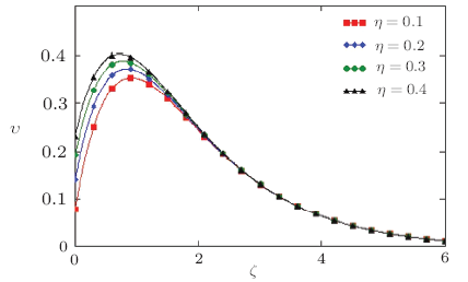
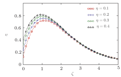
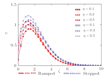
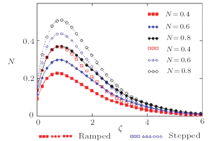
The main theme of this paper is the investigation of thermal and mass diffusion in the unsteady, slip flow of a viscous fluid having the property of incompressibility. Various numerical values of the skin-friction and velocity were calculated as function of time $\tau$ for different values of physical parameters which are Schmidt number $Sc$, Prandtl number $Pr$, slip parameter $\eta$ and buoyancy ratio parameter $N$. The influence of these parameters on ramped and constant profiles of velocity $\upsilon$, temperature $\Theta$, Concentration $\Psi$, skin-friction $C_{f}$, Nusselt number $Nu$ and Sherwood number $Sh$ are shown graphically. From the views of Figs. 1 and 2, it is clear that growing values of slip parameter accelerates the velocity of fluid in case of both ramped and stepped wall temperature. In Fig.3, we compare the impact of ramped and constant temperature corresponding to the plate on the fluids velocity. It has been noted that the velocity of fluid (free stream) for constant temperature is higher than the velocity for ramped temperature. These predictions have been illustrated in Fig.3. In order to compare the effect of ramped and constant temperature on the fluid velocity for various value of the buoyancy ratio parameter $N$, we have plotted Fig.4. We observe from Fig.4 that the motion of fluid rises for large value of buoyancy ratio parameter $N~({\rm i.e}, N> 0)$. The reason is that the mass buoyancy force acts in the same direction as the thermal buoyancy force. It is also perceived that velocity in case of constant temperature is greater than velocity in case of ramped temperature. Physically this is true because in ramped temperature case heating takes place gradually when compared to isothermal temperature case.

Fig.1

New window|Download| PPT slide
Fig.1Non-dimensional velocity outline along $\zeta$ for various values of slip parameter $\eta$ corresponding to ramped temperature of plate with $\tau=0.8$, $Pr= 0.71$, and $Sc=0.16$.

Fig.2

New window|Download| PPT slide
Fig.2Non-dimensional velocity outline for different type values of slip parameter $\eta$ corresponding to stepped temperature of the plate with $\tau=1.2$, $Pr= 0.71$, and $Sc=0.16$.

Fig.3

New window|Download| PPT slide
Fig.3Non-dimensional velocity outline for different values of slip parameter $\eta$ corresponding to stepped and ramped temperature of the plate with $\tau=3$, $Pr= 0.71$, and $Sc=2.01$.

Fig.4

New window|Download| PPT slide
Fig.4Non-dimensional velocity outline for various value of $N$ corresponding to ramped and stepped temperature of the plate with $\tau=3$, $Pr= 0.71$, and $Sc=2.01$.



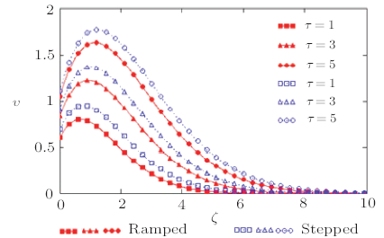
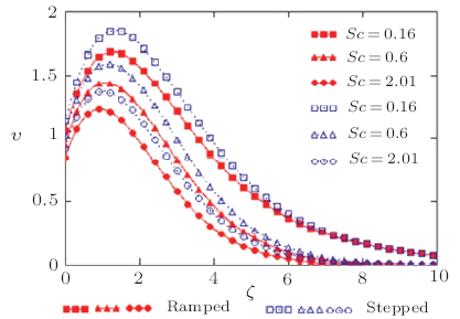
In Fig.5, we discuss the behavior of velocity for different value of time parameter $\tau$, for both the cases, that is ramped and constant temperature. When we increase time, the velocity of fluid is increased. Also in this Fig.5, we compare the effect of ramped and constant temperature. Furthermore, it has been observed that velocity of the fluid for constant temperature is comparatively higher than ramped temperature. Further analysis suggests that the fluid velocity is maximum near the plate and subsequently decreases as we move away from the plates. The motion of fluid becomes zero in particular case, where the distance possibly enlarges. Moreover the velocity is increasing function of time. Figure 6 shows that an increasing $Sc$ implies that viscous forces dominate over the diffusional effects. Schmidt number in free convection flow regimes represents the relative effectiveness momentum and mass transfer by diffusion in the velocity and concentration. Smaller values correspond to lower molecular weight species diffusing i.e. Hydrogen in air $(Sc\sim 0.16)$ and higher values to denser hydrocarbons diffusing in air i.e. Ethyl benzene in air $(Sc\sim 2.0)$. Effectively therefore if $Sc$ is increased then momentum diffusion will counteract, since viscosity effects will increase and molecular diffusivity will be reduced. The flow will therefore be decelerated with a rise in in both cases, namely ramped temperature of the plate and constant temperature of the plate as testified to by Fig.6. It also discovered that the rate of velocity in case of constant temperature is greater than in case of ramped temperature. This is expected since in the case of ramped wall temperature the heating of the fluid takes place more gradually than in the isothermal plate case. This feature is important in for example achieving better flow control in nuclear engineering applications, since ramping of the enclosing channel walls can help to decrease velocities.

Fig.5

New window|Download| PPT slide
Fig.5Non-dimensional velocity outline for various value of $\tau$ corresponding to ramped and stepped temperature of the plate with $\eta=0.9$, $Pr= 0.71$, and $Sc=2.01$.

Fig.6

New window|Download| PPT slide
Fig.6Non-dimensional velocity outline for various value of $Sc$ corresponding to ramped and stepped temperature of the plate with $\eta=0.9$, $Pr= 0.71$, and $\tau=3$.



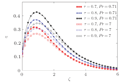
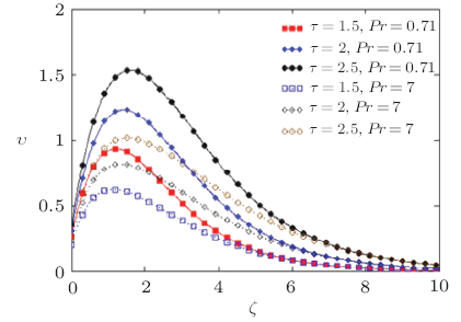
Figures 7 and 8 show the velocity of fluid in case of ramped temperature and constant temperature for different value of $\tau$ and two various values of $Pr$ i.e. $(Pr= 0.71)$ and $(Pr= 7)$.

Fig.7

New window|Download| PPT slide
Fig.7Non-dimensional velocity outline for various value of $Pr$ and $\tau$ corresponding to ramped temperature of the plate with $\eta=0.9$ and $N= 0.8$.

Fig.8

New window|Download| PPT slide
Fig.8Non-dimensional velocity outline for various value of $Pr$ and $\tau$ corresponding to stepped temperature of the plate with $\eta=0.9$ and $N= 0.8$.



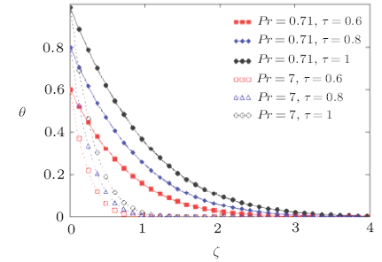
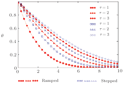
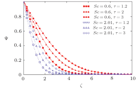
The two most frequently encountered fluids in engineering are air and water and these values of $Pr$ correspond to these two cases, respectively. This approach was established by Ostrach and Simon^[37] at NASA in the early 1950s. It is obviously follows from Figs. 7 and 8 that if we increase time then the velocity of fluid is increasing but decreasing for large value of $Pr$. Since higher $Pr$ fluids will possess greater viscosities and this will serve to reduce velocities. Furthermore from Figs. 7 and 8 that the velocity of fluid for the air $(Pr= 0.71)$ is larger than that of water $(Pr= 7)$ in both cases. These Figs. 7 and 8 clearly show that when time is zero, the velocity satisfies the initial condition given in Eq. (10). Figures 9 and 10 show the variations of temperature outline for various value of $\tau$ and for two different values of $Pr$ such as for air $(Pr= 0.71)$ and for water is $(Pr= 7)$. These analyses predict that from Figs. 9 and 10 that temperature profiles decrease if we increase the value of $Pr$ for the both cases of ramped and constant temperature of the plate. In Fig.11, we compare the variation of temperature profile in both cases, namely ramped and constant temperature of the plate. From Fig.11 it is clear that constant temperature profiles are found larger than ramped temperature profiles. In addition, it is is observed from Fig.11 that for large values of time, the temperature of the fluid is increasing in previously both cases. All the observation and result obtained from these figures are identical to the boundary condition given in Eq. (10) at temperature. Figure 12 shows the variations of concentration profile for different value of $\tau$ and for two different values of $Sc$. It is observed that concentration profiles decreases if we increase the value of $Sc$, while increases for large value of $\tau$.

Fig.9

New window|Download| PPT slide
Fig.9Non-dimensional temperature outline for different values of $Pr$ and $\tau$ corresponding to ramped temperature of the plate.

Fig.10

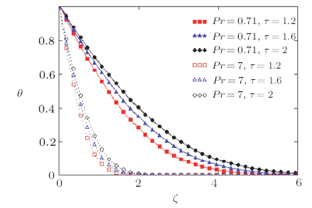New window|Download| PPT slide
Fig.10Non-dimensional temperature outline for different values of $Pr$ and $\tau$ corresponding to stepped temperature of the plate.

Fig.11

New window|Download| PPT slide
Fig.11Non-dimensional temperature outline for different values of $\tau$ and $Pr=0.71$ corresponding to ramped and stepped temperature of the plate.

Fig.12

New window|Download| PPT slide
Fig.12Non-dimensional concentration outline for different values of $Sc$ and $\tau$ corresponding to ramped temperature of the plate.



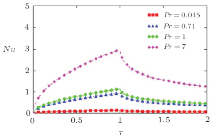
Figures 13 and 14 display the modifications of skin-friction along with time for various value of slip parameter $\eta$. Figures 13 and 14 show that if we increase the value of slip parameter $\eta$ then skin-friction is decreasing in both possible cases, discussed in previous section i.e. ramped and constant temperature of the plate. In Fig.15 we compare the modification of skin-friction in both cases namely, ramped and constant temperature plate. It is noted from Fig.15 that Modification of skin-friction in case of constant temperature plate is found smaller than ramped temperature of the plate. Figure 16 shows the modification of Sherwood number along with time $\tau$ for various value of Sc. It is clearly observed that Sherwood number is increasing for the growing value of $Sc$. Figures 17 and 18 show the modification of Nusselt number along with time $\tau$ for various value of $Pr$. Figures 17 and 18 inference that if we increase the value of $Pr$ both in cases, namely ramped temperature of the plate as well as in constant temperature of the plate then Nusselt number is increasing. It is also obviously noted that Nusselt number for mercury $(Pr=0.015)$ is smaller than air $(Pr=0.71)$, electrolytic solutions $(Pr=1)$ and for water $(Pr=7)$. These behaviors in current study have a proper agreement with the observations made in Ref. ^[33].

Fig.13

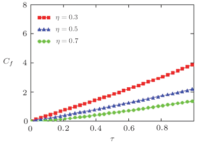New window|Download| PPT slide
Fig.13Modification of skin-friction $C_{f}$ for various value of slip parameter $\eta$ corresponding to the ramped temperature of the plate with $N=0.8$, $Pr=7$, and $Sc=2.01$.

Fig.14

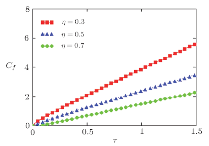New window|Download| PPT slide
Fig.14Modification of skin-friction $C_{f}$ for various value of slip parameter $\eta$ corresponding to the stepped temperature of the plate with $N=0.8$, $Pr=7$, and $Sc=2.01$.

Fig.15

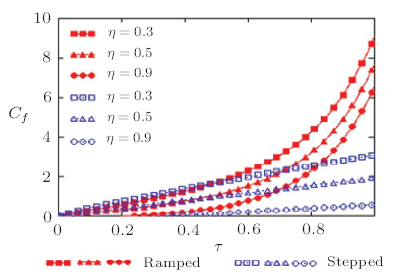New window|Download| PPT slide
Fig.15Modification of skin-friction $C_{f}$ for various value of slip parameter $\eta$ corresponding to the ramped and stepped temperature of the plate with $N=0.6$, $Pr=7$, and $Sc=2.01$.

Fig.16

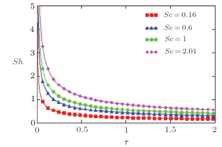New window|Download| PPT slide
Fig.16Modification of Sherwood number $Sh$ for various value of $Pr$ corresponding to stepped temperature of the plate.

Fig.17

New window|Download| PPT slide
Fig.17Modification of Nusselt-number $Nu$ for various value of $Pr$ corresponding to the ramped temperature of the plate.

Fig.18

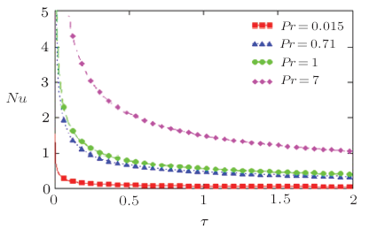New window|Download| PPT slide
Fig.18Modification of Nusselt-number $Nu$ for various value of $Pr$ corresponding to the stepped temperature of the plate.



Numerical results of skin friction, Nusselt number, and Sherwood number at the plate $(\zeta=0)$ are presented in Tables 1 to 5 for various values of slip parameter $\eta$, Prandtl number $Pr$, Schmidt number $Sc$, mass to thermal buoyancy ratio parameter $N$ and time $\tau$. It is observed from Table 1 that skin friction $C_{f}$ increases with an increase in Prandtl number $Pr$, mass to thermal buoyancy ratio parameter $N$ and time $\tau$ while the result is reversed with increase in slip parameter $\eta$ and Schmidt number $Sc$ for ramped wall temperature as well as for stepped wall temperature in Table 2. Numerical results of Nusselt number at the plate $(\zeta=0)$ are expressed in Tables 3 and 4 for different values Prandtl number $Pr$ and time $\tau$.


Table 1
Table 1Skin-friction for ramped temperature.

New window|CSV


Table 2
Table 2Skin-friction for stepped temperature.

New window|CSV


Table 3
Table 3Nusselt number for ramped temperature.

New window|CSV


Table 4
Table 4Nusselt number for stepped temperature.

New window|CSV


Table 5
Table 5Sherwood number.

New window|CSV

Table 3 shows that the Nusselt number $Nu$ which determines the rate of heat transfer at the plate increases as Prandtl number $Pr$ and time $\tau$ progresses for ramped wall temperature. It is perceived from Table 4 that the Nusselt number $Nu$ increases for large values of Prandtl number $Pr$ while the result is reversed with increase in time $\tau$ for stepped wall temperature. The rate of concentration at the surface of the wall is calculated in term of Sherwood in Table 5. It is seen that Sherwood number $Sh$ increases with an increase in Schmidt number while the result is reversed with increase in time.

6 Conclusion

Exact solutions are obtained for the wall driven flow of a viscous fluid under the influence of ramped wall temperature. Slippage over the vertical plate is not negligible. The dimensionless mathematical model for the fluid is operated with the help of Laplace transforms. Furthermore, these obtained solutions are in terms of simpler transcendental and complementary error functions. It is verified that solutions for temperature, concentration, and velocity satisfy the imposed initial and boundary conditions. The impact of involved physical parameters on the velocity field, temperature, Nusselt number and Skin friction has been examined. The entire discussion can be reduced to the following concluding remarks:

$\bullet$ Velocity increases for the large values of slip parameter.

$\bullet$ Skin friction is decreasing function of slip parameter.

$\bullet$ Increasing values of Prandtl number $Pr$ decrease the speed of fluid. Since higher $Pr$ fluids will possess greater viscosities and this will serve to reduce velocities, thereby lowering the skin friction.

$\bullet$ For the large values of Prandtl number $Pr$ the thermal diffusivity, take small space.

$\bullet$Increasing values of Schmidt number $Sc$, stops the motion of fluid. An increasing implies that viscous forces dominate over the diffusional effects. Schmidt number in free convection flow regimes represents the relative effectiveness momentum and mass transfer by diffusion in the velocity and concentration. Effectively therefore if it is increased then momentum diffusion will counteract, since viscosity effects will increase and molecular diffusivity will be reduced. The flow will therefore be decelerated with a rise in $Sc$.

$\bullet$ Relation of Schmidt number $Sc$ and skin friction are inverse.

$\bullet$ Velocity and skin friction are increasing functions of buoyancy ratio parameter. The reason is that the mass buoyancy force acts in the same direction as the thermal buoyancy force.

$\bullet$ For large values of time, the temperature of fluid rises and it moves faster. We compare the effect of ramped and stepped temperature corresponding to the plate on the fluid velocity. For this situation our result indicates that velocity in case of constant temperature is greater than in case of ramped temperature. The present results are useful in further explaining the important class of flows in which the driving force is induced by a combination of the thermal and chemical diffusion effects. Such results have immediate relevance in industrial thermofluid dynamics, transient energy systems and also buoyancy-driven geophysical and atmospheric vertical flows.

The authors have declared that no competing interests exist.

Reference View Option By original order
By published year
By cited within times
By Impact factor

[1] P. Chandran, N. C. Sacheti, A. K. Singh , Heat and Mass Transfer 41 ( 2005) 459.
[Cited within: 2]

[2] P. Chandran, N. C. Sacheti, A. K. Singh, J. Phys. Soc. Jpn. 67(1998) 124.


[3] P. Ganesan and G. Palani , Heat and Mass Transfer 39 ( 2003) 277.
[Cited within: 1]

[4] A. Hayday, D. Bowlus, R. McGraw , J. Heat Transfer 89 ( 1967) 244.
[Cited within: 1]

[5] J. Schetz, J. Appl. Mech . 30(1963) 263.
[Cited within: 1]

[6] T. Kao, Lett. Heat and Mass Transfer 2 ( 1975) 419.
[Cited within: 1]

[7] M. Kelleher , J. Heat Transfer 93 ( 1971) 349.
[Cited within: 1]

[8] S. Lee and M. Yovanovich , J. Heat Transfer. 112 ( 1991) 336.
[Cited within: 1]

[9] V. Soundalgekar , J. Heat Transfer 99 ( 1977) 499.
[Cited within: 2]

[10] D. Ingham, Int. J. Heat and Mass Transfer 21 ( 1978) 67.
[Cited within: 2]

[11] A. Singh and N. Kumar, Astrophys. Space Sci. 98(1984) 245.
[Cited within: 1]

[12] A. Gupta, I. Popp, V. Soundalgekar , Revue Roumaine des Sciences Techniques Serie de Mecanique Appliquee 24 ( 1979) 561.
[Cited within: 1]

[13] A. Raptis and A. Singh, Int. Commun. Heat and Mass Transfer 10 ( 1983) 313.
[Cited within: 2]

[14] A. R. Khaled and K. Vafai , Int.J. Non-Linear Mech. 39(2004) 795.
[Cited within: 1]

[15] E. Ashmawy, J. Egypt. Mathe . Soc. 23(2015) 563.
[Cited within: 1]

[16] M. Tahir, M. Imran, N. Raza, M. Abdullah, M. Aleem , Results in Phys. 7(2017) 1887.
[Cited within: 1]

[17] M. A. Day , Erkenntnis 33 ( 1990) 285.
[Cited within: 1]

[18] C. Navier , M$\acute{e}$moires de l'Acad$\acute{e}$mie Royale des Sciences de l'Institut de France 6 ( 1823) 389.
[Cited within: 1]

[19] R. Pit, H. Hervet , L. L$\acute{e}$ger, Tribology Lett. 7(1999) 147.
[Cited within: 1]

[20] T. D. Blake , Colloids and Surfaces 47 ( 1990) 135.
[Cited within: 1]

[21] G. Willmott , Phys. Rev. E 77 ( 2008) 055302.
[Cited within: 1]

[22] E. Ashmawy , Arch. Mech. 63(2011) 341.


[23] F. Yang , Chem. Eng. Commun. 197(2009) 544.
[Cited within: 1]

[24] N. Ghara, S. Das, S. Maji, R. Jana , Am. J. Sci. Ind. Res. 3(2012) 376.
[Cited within: 1]

[25] G. Seth, B. Kumbhakar, S. Sarkar , Int. J. Eng. Sci. Tech. 7(2015) 94.
[Cited within: 1]

[26] B. P. Reddy , Int. J. Appl. Mech. Eng. 19(2014) 303.
[Cited within: 1]

[27] Samiulhaq, S. Ahmad, D. Vieru, I. Khan, S. Shafie , PloS One 9 ( 2014) e88766.
[Cited within: 1]

[28] M. Narahari and L. Debnath , J. Appl. Mathe. Mech./Zeitschrift f$\ddot{u}$r Angewandte Mathematik und Mechanik 93 ( 2013) 38.
[Cited within: 1]

[29] M. Mansour, R. Mohamed, M. Abd-Elaziz, S. Ahmed , Int. J. Appl. Mathe. Mech. 3(2007) 99.
[Cited within: 1]

[30] V. Soundalgekar , J. Appl. Mech . 46(1979) 757.
[Cited within: 1]

[31] U. Das, S. Ray, V. Soundalgekar , Heat and Mass Transfer 31 ( 1996) 163.


[32] A. J. Chamkha, H. S. Takhar, V. Soundalgekar, J. Chem. Eng . 84(2001) 335.
[Cited within: 1]

[33] Samiulhaq, I. Khan, F. Ali, A. Khan, T. N. A. Abdelhameed , Abstr. Appl. Anal. Article ID 327975 ( 2015).
[Cited within: 4]

[34] M. Narahari, S. Tippa, R. Pendyala, M. Y. Nayan, in Proc. 11th Int. Conf. Appl. Theor. Mach. Kuala Lumpur, WSEAS Press, Malaysia, April 23-25,( 2015) 126-137..
[Cited within: 1]

[35] N. A. Shah, A. A. Zafar, S. Akhtar , Arabian J. Mathe. 7(2018) 49.
[Cited within: 1]

[36] M. Narahari, O. A . B$\acute{e}$g, and S. K. Ghosh, World
[J]. Mech. 2011 ( 2011) 176.
[Cited within: 2]

[37] S. Ostrach , An Analysis of Laminar Free-Convection Flow and Heat Transfer about a Flat Plate Parallel to the Direction of the Generating Body Force, Tech. Rep., NASA Lewis Research Center, Cleveland OH ( 1952).
[Cited within: 1]