M Qasim^,1,2,4, N Riaz², Dianchen Lu¹, S Shafie³¹Department of Mathematics, Faculty of Science, Jiangsu University, Zhenjiang 212013, China
²Department of Mathematics, COMSATS University Islamabad (CUI), 455000, Park Road, Tarlai Kalan, Islamabad, Pakistan
³Department of Mathematical Sciences, Faculty of Science, Universiti Teknologi Malaysia, 81310 UTM Johor Bahru, Johor 81310, Malaysia

First author contact: ⁴ Author to whom any correspondence should be addressed.
Received:2019-10-3Revised:2019-12-25Accepted:2019-12-25Online:2020-02-24


Abstract
In this article, three-dimensional mixed convection flow over an exponentially stretching sheet is investigated. Energy equation is modelled in the presence of viscous dissipation and variable thermal conductivity. Temperature of the sheet is varying exponentially and is chosen in a form that facilitates the similarity transformations to obtain self-similar equations. Resulting nonlinear ordinary differential equations are solved numerically employing the Runge–Kutta shooting method. In order to check the accuracy of the method, these equations are also solved using bvp4c built-in routine in Matlab. Both solutions are in excellent agreement. The effects of physical parameters on the dimensionless velocity field and temperature are demonstrated through various graphs. The novelty of this analysis is the self-similar solution of the three-dimensional boundary layer flow in the presence of mixed convection, viscous dissipation and variable thermal conductivity.
Keywords： self-similar equations;viscous dissipation;mixed convection;variable thermal conductivity;shooting technique;bvp4c Matlab


PDF (1066KB)MetadataMetricsRelated articlesExportEndNote|Ris|BibtexFavorite
Cite this article
M Qasim, N Riaz, Dianchen Lu, S Shafie. Three-dimensional mixed convection flow with variable thermal conductivity and frictional heating. Communications in Theoretical Physics, 2020, 72(3): 035003- doi:10.1088/1572-9494/ab6908

1. Introduction

Flow induced by a continuously stretching sheet in a quiescent fluid have applications in manufacturing processes of plastic films, hot rolling, glass fiber, wire drawing, paper production, extrusion, spinning of laments, production of synthetic sheets, glass fiber and paper production, extrusion, continuous casting, spinning of laments, production of synthetic sheets etc [1–10]. In convection, there is a fluid flowing relative to surface and a temperature difference between fluid and surface. In these heat convection processes, energy is transferred from a surface to fluid flowing over it as a result of temperature difference between fluid and surface. The flow over a surface is also induced by thermal buoyancy and these thermal buoyancy effects are more prominent if the surface is vertical. When the sheet is being stretched vertically with a forced velocity then buoyance forces cannot be neglected and flow in this case is mixed convective flow [11–19].

Boundary layer flow over an exponentially stretching surface is firstly investigated by Magyari and Keller [20]. Elbashbeshy [21] performed heat transfer analysis of the flow induced by a permeable exponentially stretching sheet. Sajid and Hayat [22] computed the series solution of the self-similar equations that governs the flow over an exponentially stretching sheet in the presence of linear thermal radiation by the homotopy analysis method. The effect of thermal radiation in the presence of viscous dissipation on the flow over an exponentially stretching sheet is examined by Bidin and Nazar [23]. Partha et al [24] provided the similarity solution of mixed convection flow over an exponentially stretching sheet in the presence of frictional heating. Bhattacharyya and Layek [25] investigated boundary layer flow over an exponentially stretching surface in an exponentially moving parallel free stream. Dual solutions of MHD boundary layer flow induced by an exponentially stretching sheet with non-uniform heat sink/source are analysed by Raju et al [26]. Sulochana and Sandeep [27] examined the stagnation point flow of nanofluid over an exponentially shrinking/stretching cylinder. Three-dimensional flow of viscous fluid over an exponentially stretching sheet is firstly studied by Liu et al [28]. Afridi and Qasim [29] inspected the entropy generation in three-dimensional boundary flow over an exponentially stretching surface in the presence of viscous dissipation.

All studies cited above related to flow induced by the exponentially stretching sheet with constant fluid properties. It is now well established that the physical properties of fluids may vary with temperature [30–34]. The magnitude of variation in properties varies from one fluid to another and depends on temperature limits of ambient fluid. It can be observed that the variable viscosity and thermal conductivity are quite significant for most of the fluids as compared to the variations in other properties. It is also believed that the difference between the theoretical and experimental results is because the properties of fluid are assumed to be constant and not temperature-dependent.

To best of our knowledge no one analysed the three-dimensional boundary layer flow over an exponentially stretching sheet with temperature-dependent thermal conductivity. Keeping this in mind, our aim is to analyse three-dimensional mixed convection flow induced by exponentially stretching sheet in the presence of frictional heating. The thermal conductivity of fluid is assumed to vary with temperature. Governing equations are modelled and simplified under boundary layer approximations. Modelled partial differential equations are then transformed into non-linear ordinary differential equations by utilizing similarity transformations. Special forms of stretching velocity and surface temperature varying exponentially are chosen for accurate similarity transformations. The novelty of the present study is the self-similar solution of three-dimensional boundary-layer flow in the presence of mixed convection, viscous dissipation and temperature-dependent thermal conductivity. To check the validation of our numerical code of the shooting method obtained results are also compared with Matlab boundary value solver bvp4c [35]. Effects of physical parameters of interest on velocity and temperature profile are analyzed.

2. Formulation

Three-dimensional mixed convection boundary layer flow over a sheet that is being stretched exponentially has been considered for investigation. The sheet is being stretched in both $x-$ and $y-$ directions with velocities ${u}_{w}={u}_{0}{{\rm{e}}}^{\left(\tfrac{x+y}{L}\right)}$ and ${v}_{w}={v}_{0}{{\rm{e}}}^{\left(\tfrac{x+y}{L}\right)}$ respectively. The temperature of the sheet is ${T}_{s}={T}_{a}+A{{\rm{e}}}^{2\left(\tfrac{x+y}{L}\right)}$ (A is the constant characteristic temperature) and the temperature of the ambient fluid is ${T}_{a}.$ In the presence of frictional heating the boundary layer equations for the flow and heat transfer are [28, 29]:(1)$\begin{eqnarray}\displaystyle \frac{\partial u}{\partial x}+\displaystyle \frac{\partial v}{\partial y}+\displaystyle \frac{\partial w}{\partial z}=0,\end{eqnarray}$(2)$\begin{eqnarray}u\displaystyle \frac{\partial u}{\partial x}+v\displaystyle \frac{\partial u}{\partial y}+w\displaystyle \frac{\partial u}{\partial z}=\displaystyle \frac{\mu }{\rho }\displaystyle \frac{{\partial }^{2}u}{\partial {z}^{2}}+g{\alpha }_{T}\left(T-{T}_{a}\right),\end{eqnarray}$(3)$\begin{eqnarray}u\displaystyle \frac{\partial v}{\partial x}+v\displaystyle \frac{\partial v}{\partial y}+w\displaystyle \frac{\partial v}{\partial z}=\displaystyle \frac{\mu }{\rho }\displaystyle \frac{{\partial }^{2}v}{\partial {z}^{2}},\end{eqnarray}$(4)$\begin{eqnarray}\begin{array}{l}u\displaystyle \frac{\partial T}{\partial x}+v\displaystyle \frac{\partial T}{\partial y}+w\displaystyle \frac{\partial T}{\partial z}=\displaystyle \frac{1}{\rho {S}_{p}}\left[k\left(T\right)\displaystyle \frac{{\partial }^{2}T}{\partial {z}^{2}}+\displaystyle \frac{\partial k\left(T\right)}{\partial T}{\left(\displaystyle \frac{\partial T}{\partial z}\right)}^{2}\right]\\ +\,\displaystyle \frac{\mu }{\rho {S}_{p}}\left[{\left(\displaystyle \frac{\partial u}{\partial z}\right)}^{2}+{\left(\displaystyle \frac{\partial v}{\partial z}\right)}^{2}\right],\end{array}\end{eqnarray}$along with physical boundary conditions [28, 29](5)$\begin{eqnarray}\begin{array}{rcl}u\left(x,y,0\right) & = & {u}_{0}{{\rm{e}}}^{\left(\tfrac{x+y}{L}\right)},v\left(x,y,0\right)={v}_{0}{{\rm{e}}}^{\left(\tfrac{x+y}{L}\right)},\\ w\left(x,y,0\right) & = & 0,T\left(x,y,0\right)={T}_{s}={T}_{a}+{A{\rm{e}}}^{2\left(\tfrac{x+y}{L}\right)},\end{array}\end{eqnarray}$(6)$\begin{eqnarray}\begin{array}{l}u\left(x,y,z\to \infty \right)\to 0,v\left(x,y,z\to \infty \right)\to 0,\\ T\left(x,y,z\to \infty \right)\to {T}_{a},\end{array}\end{eqnarray}$where $u,v$ and w are the components of velocity along $x-\,,\,y-$ and $z-$ axes, respectively, u₀ and v₀ are stretching parameters, μ is the dynamic viscosity, ρ is the density of fluid, g is the acceleration due to gravity, ${\alpha }_{T}$ is the thermal expansion coefficient, S_p denotes the specific heat, $k\left(T\right)$ is the thermal conductivity of the fluid, which is assumed to be temperature-dependent and take the following form [30–34]:(7)$\begin{eqnarray}k\left(T\right)={k}_{a}\left(1+\delta \left(\displaystyle \frac{T-{T}_{a}}{{T}_{s}-{T}_{a}}\right)\right),\end{eqnarray}$here δ is the variable thermal conductivity parameter.

Introducing similarity transformations$\begin{eqnarray*}\begin{array}{l}\xi =\sqrt{\displaystyle \frac{{u}_{0}}{2\nu L}}{z{\rm{e}}}^{\left(\tfrac{x+y}{2L}\right)},u={u}_{0}{{\rm{e}}}^{\left(\tfrac{x+y}{L}\right)}{F}^{{\prime} }(\xi ),\\ v={v}_{0}{{\rm{e}}}^{\left(\tfrac{x+y}{L}\right)}{G}^{{\prime} }(\xi ),\end{array}\end{eqnarray*}$(8)$\begin{eqnarray}\begin{array}{l}w=-\sqrt{\displaystyle \frac{\nu {u}_{0}}{2L}}{{\rm{e}}}^{\left(\tfrac{x+y}{2L}\right)}\left(F+\xi {F}^{{\prime} }+G+\xi {G}^{{}^{{\prime} }}\right),\\ T={T}_{a}+\left({T}_{s}-{T}_{a}\right){\rm{\Theta }}.\end{array}\end{eqnarray}$With similarity variable ξ, ${F}^{{\prime} }$ and ${G}^{{\prime} }$ being the dimensionless axial and transverse velocities, respectively, Θ is the dimensionless temperature and prime denotes the differentiation with respect to ξ. Equations $\left(1\right)\,-\,\left(4\right)$ along with boundary conditions (5) and (6) after using transformations (8) are transformed to self-similar equations(9)$\begin{eqnarray}{F}^{\prime\prime\prime }+{{FF}}^{{\prime\prime} }+{{GF}}^{{\prime\prime} }-2{F}^{{\prime} 2}-2{F}^{{\prime} }{G}^{{\prime} }+2\lambda {\rm{\Theta }}=0,\end{eqnarray}$(10)$\begin{eqnarray}{G}^{\prime\prime\prime }+{{FG}}^{{\prime\prime} }+{{GG}}^{{\prime\prime} }-2{F}^{{\prime} }{G}^{{\prime} }-2{G}^{{\prime} 2}=0,\end{eqnarray}$(11)$\begin{eqnarray}\begin{array}{l}\left(1+\delta {\rm{\Theta }}\right){{\rm{\Theta }}}^{{\prime\prime} }+\delta {{\rm{\Theta }}}^{{\prime} 2}+\Pr \left(F+G\right){{\rm{\Theta }}}^{{\prime} }\\ -\,4\Pr \left({F}^{{\prime} }+{G}^{{\prime} }\right){\rm{\Theta }}+{Ec}\Pr \left({F}^{{\prime\prime} 2}+{G}^{{\prime\prime} 2}\right)=0,\end{array}\end{eqnarray}$with boundary conditions(12)$\begin{eqnarray}\begin{array}{l}F\left(0\right)=0,{F}^{{\prime} }\left(0\right)=1,\\ G\left(0\right)=0,{G}^{{\prime} }\left(0\right)=\varepsilon ,\ \ {\rm{\Theta }}\left(0\right)=1, \\ {F}^{{\prime} }\left(\infty \right)=0,{G}^{{\prime} }\left(\infty \right)=0,\ {\rm{\Theta }}\left(\infty \right)=0.\end{array}\end{eqnarray}$Here $\varepsilon =\tfrac{{u}_{0}}{{v}_{0}}$ is velocity ratio parameter, ${Ec}=\tfrac{{u}_{0}^{2}}{{S}_{p}A}$ is Eckert number, and ${\Pr }=\tfrac{\mu {S}_{p}}{{k}_{a}}$ is Prandtl number and $\lambda =\tfrac{{{Gr}}_{x}}{{\mathrm{Re}}_{x}^{2}}=\tfrac{{gA}{\alpha }_{T}L}{{u}_{0}^{2}}$ is the mixed convection parameter.

3. Solution methodologies

3.1. Shooting method

In order to solve self-similar non-linear equations (9)–(11) along with boundary conditions (11) are solved numerically by the Runge–Kutta shooting method, the boundary value problem is firstly converted into initial value problem by letting(13)$\begin{eqnarray}\begin{array}{rcl}{e}_{1} & = & F,{e}_{2}={e}_{1}^{{\prime} }={F}^{{\prime} },{e}_{3}={e}_{2}^{{\prime} }={F}^{{\prime\prime} },{e}_{4}=G,{e}_{5}={e}_{4}^{{\prime} }\\ & = & {G}^{{\prime} },{e}_{6}={e}_{5}^{{\prime} }={G}^{{\prime\prime} },{e}_{7}={\rm{\Theta }},{e}_{8}={e}_{7}^{{\prime} }={{\rm{\Theta }}}^{{\prime} }.\end{array}\end{eqnarray}$Incorporating equation (13) into equations (9)–(11), we get following system of first-order equations(14)$\begin{eqnarray}\left(\begin{array}{c}{e}_{1}^{{\prime} }\\ {e}_{2}^{{\prime} }\\ {e}_{3}^{{\prime} }\\ {e}_{4}^{{\prime} }\\ {e}_{5}^{{\prime} }\\ {e}_{6}^{{\prime} }\\ {e}_{7}^{{\prime} }\\ {e}_{8}^{{\prime} }\end{array}\right)=\left(\begin{array}{c}{e}_{2}\\ {e}_{3}\\ -{e}_{1}{e}_{3}-{e}_{4}{e}_{3}+2{e}_{2}{e}_{2}+2{e}_{2}{e}_{5}-2\lambda {e}_{7}\\ {e}_{5}\\ {e}_{6}\\ -{e}_{1}{e}_{6}-{e}_{4}{e}_{6}+2{e}_{5}{e}_{5}+2{e}_{2}{e}_{5}\\ {e}_{8}\\ \frac{1}{1+\delta {e}_{7}}\left[4\Pr \left({e}_{2}+{e}_{5}\right){e}_{7}-\Pr \left({e}_{1}+{e}_{4}\right){e}_{8}-\Pr {Ec}\left({e}_{3}{e}_{3}+{e}_{6}{e}_{6}\right)-\delta {e}_{8}{e}_{8}\right]\end{array}\right),\end{eqnarray}$with initial conditions(15)$\begin{eqnarray}\left(\begin{array}{c}{e}_{1}\left(0\right)\\ {e}_{2}\left(0\right)\\ {e}_{3}\left(0\right)\\ {e}_{4}\left(0\right)\\ {e}_{5}\left(0\right)\\ {e}_{6}\left(0\right)\\ {e}_{7}\left(0\right)\\ {e}_{8}\left(0\right)\end{array}\right)=\left(\begin{array}{c}0\\ 1\\ {q}_{1}\\ 0\\ \varepsilon \\ {q}_{2}\\ 1\\ {q}_{3}\end{array}\right).\end{eqnarray}$The shooting scheme is applied to find the missing initial conditions to guess q₁, q₂ and q₃ until the conditions ${F}^{{\prime} }\left(\infty \right)=0,{G}^{{\prime} }\left(\infty \right)=0$ and $\ \ {\rm{\Theta }}\left(\infty \right)=0$ are satisfied. After finding these missing conditions, the system of the first-order ordinary differential equation (14) is solved by the Runge–Kutta method.

3.2. Bvp4c

The numerical solutions are also computed by using Matlab built-in boundary value solver bvp4c. Matlab code bvp4c for the two-point boundary value problem is a finite difference code based on three-stage collocation at Lobatto points. These collocation polynomials provide a ${C}^{1}$-continuous solution, which is fourth order uniformly accurate in the interval of integration. Mesh selection and error control are based on the residual of the continuous solution. The collocation method routines a mesh of points to divide the interval of integration into subintervals. The solver computed a numerical solution by solving a global system of algebraic equations resulting from the boundary conditions and the collocation conditions imposed on all the subintervals. The solver then estimates the error of obtained numerical solution on each subinterval. The solver adapts the mesh and repeats the process, until the solution satisfies the tolerance criteria [35].

3.3. Code validation

The comparison between the shooting method and bvp4c is presented in table 1 for the validation of our numerical codes. Moreover, table 2 shows the comparison of present results with the existing study. The attained results are found to be in excellent agreement.


Table 1.
Table 1.Effects of different physical parameters on ${F}^{{\prime\prime} }\left(0\right),-{G}^{{\prime\prime} }\left(0\right),$ ${{\rm{\Theta }}}^{{\prime\prime} }\left(0\right)$ and comparison between shooting method and built-in routine bvp4c in Matlab.

					$-{F}^{{\prime\prime} }\left(0\right)$		$-{G}^{{\prime\prime} }\left(0\right)$		$-{{\rm{\Theta }}}^{{\prime} }\left(0\right)$
λ	${\Pr }$	Ec	δ	ϵ	Shooting	bvp4c	Shooting	bvp4c	Shooting	bvp4c
0.0	1.2	0.6	0.2	0.5	1.569 89	1.569 62	0.784 94	0.784 75	1.823 65	1.823 55
0.5	1.2	0.6	0.2	0.5	1.271 68	1.271 24	0.806 53	0.806 12	1.932 93	1.932 77
1.0	1.2	0.6	0.2	0.5	0.996 57	0.996 18	0.823 76	0.823 45	2.015 22	2.015 09
1.5	1.2	0.6	0.2	0.5	0.735 65	0.735 44	0.838 61	0.838 36	2.080 27	2.080 11
1.2	0.3	0.6	0.2	0.5	0.591 71	0.591 49	0.865 19	0.864 87	1.007 37	1.007 23
1.2	0.7	0.6	0.2	0.5	0.773 96	0.773 64	0.843 76	0.843 42	1.556 59	1.556 41
1.2	1.2	0.6	0.2	0.5	0.890 79	0.890 47	0.829 93	0.829 78	2.042 99	2.042 81
1.2	6.7	0.6	0.2	0.5	1.171 19	1.170 98	0.803 08	0.802 73	4.752 33	4.752 02
1.2	1.0	0.0	0.2	0.5	0.892 27	0.892 06	0.829 71	0.829 65	2.033 36	2.033 22
1.2	1.0	1.0	0.2	0.5	0.827 28	0.826 95	0.837 35	0.837 19	1.760 31	1.760 17
1.2	1.0	2.0	0.2	0.5	0.771 27	0.771 13	0.843 79	0.843 52	1.524 76	1.524 61
1.2	1.0	3.0	0.2	0.5	0.722 07	0.721 95	0.849 35	0.849 14	1.316 99	1.316 71
1.2	1.0	0.5	0.0	0.5	0.887 74	0.887 55	0.830 98	0.830 65	2.129 88	2.129 69
1.2	1.0	0.5	1.0	0.5	0.765 63	0.765 48	0.843 08	0.842 88	1.375 84	1.375 77
1.2	1.0	0.5	2.0	0.5	0.683 16	0.683 03	0.852 15	0.851 94	1.081 84	1.081 69
1.2	1.0	0.5	3.0	0.5	0.622 25	0.622 11	0.859 14	0.858 92	0.916 69	0.916 52

New window|CSV


Table 2.
Table 2.Comparison between our numerical results and the results of Liu et al [28] for ${F}^{{\prime\prime} }\left(0\right)\,$ and ${G}^{{\prime\prime} }\left(0\right)$ in the case where $\lambda =0,\delta =0,{Ec}=0.$

	$-{F}^{{\prime\prime} }\left(0\right)$		$-{G}^{{\prime\prime} }\left(0\right)$
ϵ	[28]	Present	[28]	Present
0.0	1.281 808 56	1.281 808 56	0.784 944 23	0.784 944 23
0.5	1.569 888 46	1.569 888 47	0.000 000 0	0.000 000 0
1.0	1.812 751 05	1.812 751 05	1.812 751 05	1.812 751 05

New window|CSV

4. Results and discussion

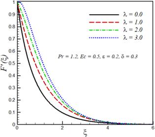
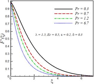
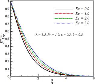
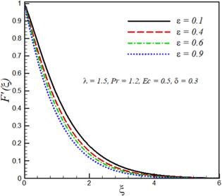
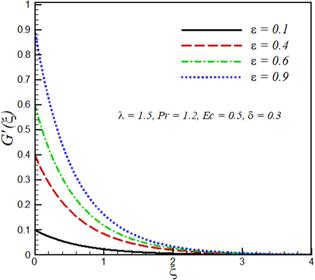
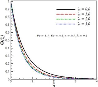
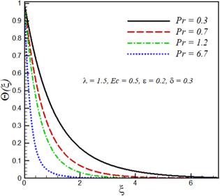
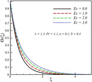
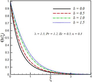
The effects of mixed convection parameter λ, Prandtl number $\Pr $ Eckert number Ec, velocity ratio parameter ϵ and variable thermal conductivity parameter δ on velocity components ${F}^{{\prime} }\left(\xi \right),$ ${G}^{{\prime} }\left(\xi \right)$ and temperature ${\rm{\Theta }}\left(\xi \right)$ are investigated. This purpose is achieved by plotting figures 1–9. The effect of the mixed convection parameter on velocity ${F}^{{\prime} }\left(\xi \right)$ is seen in figure 1. Velocity ${F}^{{\prime} }\left(\xi \right)$ increases by increasing $\lambda .$ For large λ, there is a stronger buoyancy force due to which momentum boundary layer increases. The influence of Prandtl number $\Pr $ on velocity ${F}^{{\prime} }\left(\xi \right)$ is displayed in figure 2. The large values of Prandtl number $\Pr $ correspond to stronger momentum and weaker thermal diffusivity, which therefore reduces the thermal boundary layer thickness. Figure 3 explicates the effect of Eckert number Ec on the velocity As expected velocity increases by increasing ${Ec}.$ Figure 4 illustrates that velocity ${F}^{{\prime} }\left(\xi \right)$ decreases by increasing velocity ratio parameter ϵ whereas velocity ${G}^{{\prime} }\left(\xi \right)$ increases by increasing velocity ratio parameter ϵ (see figure 5). Temperature and thermal boundary layer decreases upon increasing mixed convection parameter λ (see figure 6). Increasing the buoyancy parameter specifies the higher temperature from the surface relative to ambient, therefore thermal boundary layer decreases. The influence of Prandtl number $\Pr $ on the temperature field is illustrated in figure 7. The increase in the Prandtl number $Pr$ indicates a reduction in the thermal conductivity of the fluid and because of this reduction, the penetration depth of the thermal energy decreases, therefore temperature of the fluid decreases. Figure 8 shows that temperature distribution and thermal boundary layer thickness increases with an increase in Eckert number ${Ec}.$ Physically, by increasing friction between the adjacent layers of fluid increases and the kinetic energy of fluid is converted into thermal energy, which in turn rises the fluid temperature. The influence of the thermal conductivity parameter $\delta \ $ on the temperature profile is portrayed in figure 9. It is observed that the temperature of the fluid in the boundary layer increases by increasing the value of the variable thermal conductivity parameter δ. Physically, as the thermal conductivity parameter increases, the thermal conductivity of the fluid increases and, as a result, the thermal energy of fluid increases, resulting in an increase in temperature. Table 1 shows that skin friction coefficients along $-{F}^{{\prime\prime} }\left(0\right)$ transverse direction decreases by increasing mixed convection parameter λ, whereas $-{G}^{{\prime\prime} }\left(0\right)$ and local Nusselt number $-{{\rm{\Theta }}}^{{\prime} }\left(0\right)$ increases with increasing mixed convection parameter $\lambda .$ Skin friction coefficients and local Nusselt number decreases by increasing the variable thermal conductivity parameter. $-{F}^{{\prime\prime} }\left(0\right)$ and $-{{\rm{\Theta }}}^{{\prime} }\left(0\right)$ are decreasing functions of Eckert number Ec whereas increasing functions of Prandtl number ${\Pr }.$

Figure 1.

New window|Download| PPT slide
Figure 1.Effects of mixed convection parameter λ on velocity ${F}^{{\prime} }\left(\xi \right).$

Figure 2.

New window|Download| PPT slide
Figure 2.Effect of Prandtl number $\Pr $ on velocity ${F}^{{\prime} }\left(\xi \right).$

Figure 3.

New window|Download| PPT slide
Figure 3.Effect of Eckert number Ec on velocity ${F}^{{\prime} }\left(\xi \right).$

Figure 4.

New window|Download| PPT slide
Figure 4.Effect of velocity ratio parameter ϵ on velocity ${F}^{{\prime} }\left(\xi \right).$

Figure 5.

New window|Download| PPT slide
Figure 5.Effect of velocity ratio parameter ϵ on velocity ${G}^{{\prime} }\left(\xi \right).$

Figure 6.

New window|Download| PPT slide
Figure 6.Effect of mixed convection parameter λ on temperature profile ${\rm{\Theta }}\left(\xi \right).$

Figure 7.

New window|Download| PPT slide
Figure 7.Effect of Prandtl number $\Pr $ on temperature profile ${\rm{\Theta }}\left(\xi \right).$

Figure 8.

New window|Download| PPT slide
Figure 8.Effect of Eckert number Ec on temperature profile ${\rm{\Theta }}\left(\xi \right).$

Figure 9.

New window|Download| PPT slide
Figure 9.Effect of variable thermal conductivity parameter δ on temperature profile ${\rm{\Theta }}\left(\xi \right).$

5. Closing remarks

From the current analysis, the following specific conclusions are deduced:•The problem is self-similar in the presence mixed convection as well as viscous dissipation for a special type of surface temperature.
•The mixed convection parameter increases the velocity profile, but it decreases the temperature profile in the boundary layer region.
•Velocity component ${F}^{{\prime} }$ in the transverse direction and dimensionless temperature Θ decreases by increasing the Prandtl number, whereas both are decreasing functions of the Eckert number.
•Velocity decreases ${F}^{{\prime} }$ whereas ${G}^{{\prime} }$ increases by increasing the velocity ratio parameter.
•Temperature profile increases by increasing the variable thermal conductivity parameter.

Reference View Option By original order
By published year
By cited within times
By Impact factor

[1]Salleh M Z Nazar R Pop I 2010 Boundary layer flow and heat transfer over a stretching sheet with Newtonian heating
Journal of Taiwan Institute of Chemical Engineering 41 651655
DOI:10.1016/j.jtice.2010.01.013 [Cited within: 1]

[2]Turkyilmazoglu M 2011 Analytic heat and mass transfer of the mixed hydrodynamic/thermal slip MHD viscous flow over a stretching sheet
Int. J. Mech. Sci. 53 886896
DOI:10.1016/j.ijmecsci.2011.07.012

[3]Makinde O D Aziz A 2011 Boundary layer flow of a nanofluid past a stretching sheet with a convective boundary condition
Int. J. Therm. Sci. 50 13261332
DOI:10.1016/j.ijthermalsci.2011.02.019

[4]Turkyilmazoglu M Pop I 2013 Exact analytical solutions for the flow and heat transfer near the stagnation point on a stretching/shrinking sheet in a Jeffrey fluid
Int. J. Heat Mass Transfer 57 8288
DOI:10.1016/j.ijheatmasstransfer.2012.10.006

[5]Sheikholeslami M Ganji D D 2014 Heated permeable stretching surface in a porous medium using nanofluids
Journal of Applied Fluid Mechanics 7 535542


[6]Khan W A Makinde O D 2014 MHD nanofluid bioconvection due to gyrotactic microorganisms over a convectively heat stretching sheet
Int. J. Therm. Sci. 81 118124
DOI:10.1016/j.ijthermalsci.2014.03.009

[7]Rashidi M M Abdul A K Hakeem Vishnu N Ganesh Ganga B Sheikholeslami M Momoniat E 2016 Analytical and numerical studies on heat transfer of a nanofluid over a stretching/shrinking sheet with second-order slip flow model
International Journal of Mechanical and Materials Engineering 11 19
DOI:10.1186/s40712-016-0054-2

[8]Hsiao K L 2017 Micropolar nanofluid flow with MHD and viscous dissipation effects towards a stretching sheet with multimedia feature
Int. J. Heat Mass Transfer 112 983990
DOI:10.1016/j.ijheatmasstransfer.2017.05.042

[9]Rashidi M M Abbas M A 2017 Effect of slip conditions and entropy generation analysis with an effective Prandtl number model on a nanofluid flow through a stretching sheet
Entropy 19 414
DOI:10.3390/e19080414

[10]Turkyilmazoglu M 2017 Magnetohydrodynamic two-phase dusty fluid flow and heat model over deforming isothermal surfaces
Phys. Fluids 29 013302
DOI:10.1063/1.4965926 [Cited within: 1]

[11]Chamkha A J Issa C 1999 Mixed convection effects on unsteady flow and heat transfer over a stretched surface
Int. Commun. Heat Mass Transfer 26 717728
DOI:10.1016/S0735-1933(99)00058-5 [Cited within: 1]

[12]Hsiao K L 2008 MHD mixed convection of viscoelastic fluid over a stretching sheet with Ohmic dissipation
Journal of Mechanics 24 2934
DOI:10.1017/S1727719100002343

[13]Prasad K V Vajravelu K Datti P S 2010 Mixed convection heat transfer over a non-linear stretching surface with variable fluid properties
Int. J. Non Linear Mech. 45 320330
DOI:10.1016/j.ijnonlinmec.2009.12.003

[14]Turkyilmazoglu M 2013 The analytical solution of mixed convection heat transfer and fluid flow of a MHD viscoelastic fluid over a permeable stretching surface
Int. J. Mech. Sci. 77 263268
DOI:10.1016/j.ijmecsci.2013.10.011

[15]Ellahi R Hassan M Zeeshan A 2016 Aggregation effects on water base Al2O3–nanofluid over permeable wedge in mixed convection
Asia-Pac. J. Chem. Eng. 11 179186
DOI:10.1002/apj.1954

[16]Sheikholeslami M Mustafa M T Ganji D D 2016 Effect of Lorentz forces on forced convection nanofluid flow over a stretched surface
Particuology 26 108113
DOI:10.1016/j.partic.2016.01.001

[17]Ellahi R Hassan M Zeeshan A 2017 Shape effects of spherical and nonspherical nanoparticles in mixed convection flow over a vertical stretching permeable sheet
Mech. Adv. Mater. Struct. 24 12311238
DOI:10.1080/15376494.2016.1232454

[18]Afridi M I Qasim M Khan I Shafie S Alshomrani A S 2017 Entropy generation in magnetohydrodynamic mixed convection flow over an inclined stretching sheet
Entropy 19 111
DOI:10.3390/e19010010

[19]Turkyilmazoglu M 2018 Analytical solutions to mixed convection MHD fluid flow induced by a nonlinearly deforming permeable surface
Commun. Nonlinear Sci. Numer. Simul. 63 373379
DOI:10.1016/j.cnsns.2018.04.002 [Cited within: 1]

[20]Magyari E Keller B 1999 Heat and mass transfer over an exponentially stretching continuous surface
J. Phys. D: Appl. Phys. 32 577585
DOI:10.1088/0022-3727/32/5/012 [Cited within: 1]

[21]Elbashbeshy E M A 2001 Heat transfer over an exponential stretching continuous surface with suction
Arch. Mech. 53 643651
[Cited within: 1]

[22]Sajid M Hayat T 2008 Influence of thermal radiation on the boundary layer flow due to an exponentially stretching sheet
Int. Commun. Heat Mass Transfer 35 347356
DOI:10.1016/j.icheatmasstransfer.2007.08.006 [Cited within: 1]

[23]Bidin B Nazar R 2009 Numerical solution of the boundary layer flow over an exponentially stretching sheet with thermal radiation
European Journal of Scientific Research 33 710717
[Cited within: 1]

[24]Partha M K Murthy P V S N Rajasekhar G P 2005 Effect of viscous dissipation on mixed convection heat transfer from an exponentially stretching surface
Heat Mass Transfer 41 360366
DOI:10.1007/s00231-004-0552-2 [Cited within: 1]

[25]Bhattacharyya K Layek G C 2014 Thermal boundary layer in flow due to an exponentially stretching surface with an exponentially moving free stream
Modelling and Simulation in Engineering 2014 785049
DOI:10.1155/2014/785049 [Cited within: 1]

[26]Raju C S K Sandeep N Sulochana C Babu M J 2016 Dual solutions of MHD boundary layer flows pas an exponentially stretching sheet with non-uniform heat source/sink
Journal of Applied Fluid Mechanics 9 555563
DOI:10.18869/acadpub.jafm.68.225.24784 [Cited within: 1]

[27]Sulochana C Sandeep N 2016 Stagnation point flow and heat transfer behavior of Cu- water nanofluid towards horizontally and exponentially stretching/shrinking cylinder
Applied Nanosciences 6 108113
[Cited within: 1]

[28]Liu I C Wang H H Peng Y F 2013 Flow and heat transfer for three-dimensional flow over an exponentially stretching surface
Chem. Eng. Commun. 200 253268
DOI:10.1080/00986445.2012.703148 [Cited within: 3]

[29]Qasim M Afridi M I 2018 Effects of energy dissipation and variable thermal Conductivity on entropy generation rate in mixed convection flow
Journal of Thermal Science and Engineering Applications 10 044501
DOI:10.1115/1.4038703 [Cited within: 3]

[30]Chaim T C 1998 Heat transfer in a fluid with variable thermal conductivity over stretching sheet
Acta Mech. 129 6372
DOI:10.1007/BF01379650 [Cited within: 2]

[31]Chaim T C 1996 Heat transfer with variable conductivity in a stagnation-point flow towards a stretching sheet
Int. Commun. Heat Mass Transfer 23 239248
DOI:10.1016/0735-1933(96)00009-7

[32]Prasad K V Vajravelu K Datti P S 2010 Mixed convection heat transfer over a non-linear stretching surface with variable fluid properties
Int. J. Non Linear Mech. 45 320330
DOI:10.1016/j.ijnonlinmec.2009.12.003

[33]Hayat T Shehzad S A M Qasim Alsaedi A 2014 Mixed convection flow by a porous sheet with variable thermal conductivity and convective boundary condition
Braz. J. Chem. Eng. 31 113
DOI:10.1590/S0104-66322014000100011

[34]Hussain Q Asghar S Hayat T Alsaedi A 2015 Heat transfer analysis in peristaltic flow of mhd jeffrey fluid with variable thermal conductivity
J. Appl. Math. Mech. 9 0151926
DOI:10.1007/s10483-015-1926-9 [Cited within: 2]

[35]Kierzenka J Shampine L F 2001 A BVP solver based on residual control and the MATLAB PSE
ACM Transactions in Mathematics and Software 27 299316
DOI:10.1145/502800.502801 [Cited within: 2]