 ,*Laboratory of Condensed Matter Physics, Faculty of Sciences Ben M'sik, Hassan II University of Casablanca,BP 7955,Casablanca, Morocco
Corresponding authors: * E-mail:mohamed.elhafidi@univh2c.ma
Received:2019-04-12Online:2019-11-1

Abstract
Keywords:
PDF (3349KB)MetadataMetricsRelated articlesExportEndNote|Ris|BibtexFavorite
Cite this article
Abderrazak Boubekri, Moulay Youssef El Hafidi, Mohamed El Hafidi. Magnetocaloric Effect in Anisotropic Mixed Spin ½—1 System: Pair Approximation Method. [J], 2019, 71(11): 1370-1378 doi:10.1088/0253-6102/71/11/1370
1 Introduction
In recent years, the study of the magnetic properties of two-sublattices of the mixed Ising systems has attracted considerable attention. Since such systems are important for technological applications, one can observe new behaviours and phenomena in these systems, which have less translational symmetry, such as the tricritical points and the re-entrant phenomenon, which are not observed in a single spin system.Most researches have been devoted to mixed spin systems consisting of spin-1/2 and spin-S (S$>$1/2). These investigations have been carried out by a variety of methods, namely mean-field approximation (MFA),[1] effective field theory (EFT),[2-3] Monte Carlo simulation,[4] Pair approximation[5-7] and exact method.[8-9] In their paper, Dakhama et al.[10] have argued that the presence of second-nearest neighbour interactions is essential for the occurrence of a compensation point, for ferrimagnetic models.
Besides, some authors have studied the diluted mixed Ising system with different kinds of dilution methods. In the work of Xin et al.,[11-12] the authors investigated the properties of mixed spin system by using the effective field theory (EFT), when the two sublattices $A$ and $B$ are diluted independently with concentrations $p_{A}$ and $p_{B}$, which means that the site occupied by magnetic atoms in sublattice $A$ has a mean concentration 0$<p_{A}\leq$1 whereas the site occupied by magnetic atoms in sublattice $B$ has a concentration 0$<p_{B}\leq$1. The authors found that the re-entrant phenomena and two compensation points appear for certain ranges of $D/J$. The same kind of dilution method has been used by Bobak et al.[13] where the crystalline fied $D/J_{z}$ is ignored, while Benyoussef et al.[14] used another type of dilution approach. In their last model, the two sublattices are diluted with the same concentration $p$.
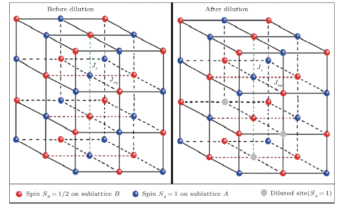
In the present paper, we consider a system of two sublattices $A$ and $B$ respectively, consisting of spin-1 and spin-1/2, independently diluted. Our investigation will be made for the system where the sublattice $A$ is diluted (0.25$\leq p_{A}\leq$1), while the sublattice $B$ is not diluted (thus, in this work $p_{B}$=1), as it is displayed in (Fig. 1). The spin-1 atoms are subjected to the local single-ion anisotropy. Thus, we examine the effects of single-ion anisotropy and dilution on the magnetic and magnetocaloric properties of the mixed diluted system, with Heisenberg ferromagnetic model, by the use of pair approximation method (PA).[15-16]
Fig. 1
 New window|Download| PPT slide
Fig. 1(Color online) A schematic view of the magnetic mixed spin system in a cubic lattice, consisting of two sublattices $A$ and $B$ with spin $S_A$=1 and $S_B$=1/2. The exchange interactions for $z$ spin direction and ($x, y$) plane are respectively $J_z$ (green dashed line) and $J_{xy}$ (brown dashed line). The dilution is restricted to $S_A$ sites.
We are here interested in studying the magnetocaloric effect with diluted mixed spin system. This effect attracted great interest in the last two decades through several published papers dealing with this topic both theoretically and experimentally.[17-23] This phenomenon has been observed in the first time by Warburg;[24] it was characterized by the heating or cooling of the magnetic materials when these are submitted to external magnetic field change.
The use of such effect allows us to benefit from refrigeration. Actually, this new technology of magnetic cooling is considered as one of promising alternatives to substitute conventional systems using greenhouse gases, since it is energy-efficient and environmentally friendly. However, researchers, all over the world, are looking for magnetic materials whether they are alloys or composites displaying a giant magnetocaloric effect in order to improve the cooling capacity. Thus, up to now, the magneto-refrigeration technology remains experimental and has not yet reached the stage of wide commercialization.
The magnetocaloric performance of materials can be assessed by the isothermal entropy change $(\Delta{S_M})$ and the refrigerant capacity (RC) as a function of the temperature and external magnetic field. These parameters can provide key information about the cooling efficiency of such materials.
The use of mixed spin systems or magnetic phase mixtures such as composites provide a potentially interesting route to the engineering of materials that might produce improved and tuned magnetic properties to satisfy the specific requirements for the magnetorefrigeration applications,
In such systems, it is well known, that the first order component gives a larger $\Delta S_M$ due to the extra contribution from latent heat, while the second order component presents a large phase transition temperature. Thus, by combining a first-order and a second-order in a single material, one should go to broaden the transition temperature and thereafter expand the region MCE.
In Mn$_{3}$GaC for example, characterized by the first order transition, one can transform it to the second order type by introducing vacancies at carbon positions or substitution of Co at Mn sites, leading to a large region of the MCE.[25-26]
The Mn$_{3}$CuN shows a large magnetic entropy change ($\Delta S_{M}$=13.5 J/kgK) but small relative cooling power (RCP=38.9 J/kg) during the first order magnetic phase transition. The researchers found that substitution of Fe for Cu sites broadened the phase transition temperature (Mn$_{3}$Cu$_{1-x}$Fe$_{x}$N[27]) and enhanced the relative cooling and reduced the effective hysteresis.
Yet, in this work, we aim to investigate the magnetocaloric properties of the anisotropic Heisenberg model, focusing on the single-ion anisotropy and the dilution effects on the entropy change ($\Delta S$) and the RCP in a mixed spin 1/2 and 1 ferromagnetic system. The rest of this paper is planned as follows: in Sec. 2, we outline the theoretical approach and we establish the expressions of different useful physical variables. In Sec. 3, we present our numerical results obtained for different values of the ionic anisotropy strength and magnetic ion concentrations. We end with a conclusion and some relevant reflections about the properties of the best magnetic materials that would give a significantly higher cooling capacity.
2 Theoretical Approach
We consider a two-sublattice mixed-spin Heisenberg system; the sites of sublattice $A$ are occupied by spins $S_{iA}$=1 and the sites of sublattice $B$ are occupied by spins $S_{jB}$=1/2; with a crystal field interaction $D$ defined on a three-dimensional lattice ($z$=6), under an additional external magnetic field and described by the following Hamiltonian:$S_{iA}$ and $S_{iB}$ refer to spins 1 and 1/2 located on sublattices $A$ and $B$, respectively. $h=-g\mu_BH$ is the external magnetic field. $J_{z}$ and $J_{xy}$ are the exchange interaction between nearest neighbors for $z$ spin direction and for ($x, y$) plane respectively. The interaction between ions $A$ and $B$ is ferromagnetic ($J_{z}, J_{xy} >$ 0). $\xi_i^A$ (respectively $\xi_j^B$) is a random variable which takes the value 1 or 0, depending on whether the site $i (j)$ is occupied by a magnetic atom of type $A (B)$ with a probability $p_{A}$ (or $p_{B}$) or not (with a probability 1 — $p_A$ (or 1 — $p_{B}$)). Here, the probabilities $p_{A}$ and $p_{B}$ can be changed independently.
2.1 Pair Approximation Approach
In the PA formalism, we start by obtaining the single spin and pair Hamiltonians $H_{ij}$ and $H_{i}$, which can be written for our particular system as follows:[15-16]For the "Pair site Hamiltonian"
for the "Single site Hamiltonian" corresponding to the sublattice $A$ or $B$ respectively. Here $z$ is the coordination number and $\lambda_{A}$, $\lambda_{B}$ are variational parameters related to molecular fields acting on the two different spins, which have obvious physical meaning.[15]
The pair Hamiltonian (2) can be presented in the form of 6$\times{}$6 matrices, being the sum of outer products, and then one has to solve the eigenvalues equation:
Thus, the calculated eigenvalues are formulated as follows:
where we have put $\Lambda_A=(z-1)p_B\lambda_B+h$ and $\Lambda_B=(z-1)p_A\lambda_A+h$.
The total free energy is stated by the following equation:[5]
In case of randomly diluted system, the Gibbs energy should be averaged over configurations with this new form:
where $G_{A}$, $G_{B}$ and $G_{AB}$ are respectively the single site energy for sublattices $A$ and $B$ and the pair site energy:
In order to formulate the problem on Pair Approximation, the partition function is calculated. Its expression reads:[28]
$$w_1=\sqrt{{\left[\left(\frac{J_z}{2}+{\Lambda{}}_A-{\Lambda{}}_B\right)-D\right]}^2+2J_{xy}^2}, $$
$$w_2=\sqrt{{\left[\left(\frac{J_z}{2}-{\Lambda{}}_A+{\Lambda{}}_B\right)-D\right]}^2+2J_{xy}^2}, $$
where $\Lambda_A=(z-1)p_B\lambda_B+h$ and $\Lambda_B=(z-1)p_A\lambda_A+h$. We can get all the thermodynamic properties such as magnetization, entropy, magnetic specific heat from the total free energy.
We must also determine the values of the parameter $\lambda_{\mu}$ ($\mu$ = $A$ or $B$) from the equilibrum condition, in which the free energy reaches its minimum in the equilibrum state:
Thus, one can obtain the total magnetization per site of the system by magnetic field derivative of energy:
leading to the formula:
With the average sublattice magnetization per site are given by:
where $\langle\cdots\rangle$ and $\langle\cdots\rangle_r$ denote the thermal and random averages, $m_{A}$ and $m_{B}$ are respectively the magnetization per site of the sublattice $A$ and $B$.
In a similar way, we can find the entropy per site $S$ from the equation
After some mathematical manipulations, the entropy magnetic is given explicitly by:
where
where
$$\begin{eqnarray*} A=2e^{\beta({J_{//}}/{2}+D)}\Big[\left(\frac{J_{//}}{2}+D\right)\Big]\cosh{\left[\beta{} \left(\frac{{\Lambda}_b}{2}+{\Lambda}_a\right)\right]}+\left(\frac{{\Lambda{}}_b}{2} +{\Lambda{}}_a\right){\rm sinh}\Big[\beta\left(\frac{{\Lambda{}}_b}{2}+{\Lambda}_b\right)\Big],\\ B=2e^{-\beta({J_{//}}/{2}\ +{\Lambda}_a-D)}\Big[-\left(\frac{J_{//}}{2}+{\Lambda}_a -D\right)\Big]\cosh{\left[\beta{}\left(\frac{w_1}{2}\right)\right]}+w_1 \sinh\Big[\beta\left(\frac{w_1}{2}\right)\Big],\\ C=2e^{-\beta{}({J_{//}}/{2}-{\Lambda}_a-D)}\Big[-\left(\frac{J_{//}}{2}-{\Lambda{}}_a-D\right)\Big] \cosh{\left[\beta{}\left(\frac{w_2}{2}\right)\right]}+w_2 \sinh\Big[\beta\left(\frac{w_2}{2}\right)\Big]. \end{eqnarray*} $$
In order to describe the magnetocaloric properties, we have to calculate the magnetic entropy change, during the isothermal demagnetization process between the external field $h>$0 and $h$=0, which is given by the Maxwell relation:
Let note that the positive value of $-\Delta S_M(T)$ corresponds to direct MCE, whereas the opposite case of heating ($-\Delta S_M(T)<$0) is called the inverse MCE and the measure of performance of a substance can be calculated through this formula of refrigeration capacity:
Another important magnetocaloric parameter is the Gruneisen ratio, which is defined as temperature change versus magnetic field under adiabatic process:[29]
The magnetic Gruneisen ratio can be conquered experimentally, and it usually exhibits a divergence toward critical temperature in magnetic materials.[30-32]
3 Numerical Results and Discussion
3.1 Magnetic Properties
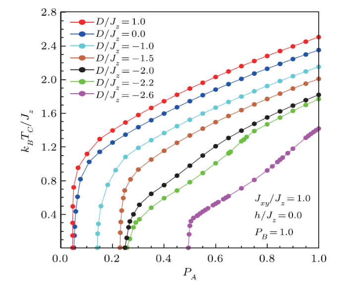
At the beginning, we present the numerical results concerning the phase diagram of a mixed diluted binary system of spin-1 and 1/2, with Heisenberg anisotropic model on the ($p_{A}, k_{B} T_{c}/J_{z}$) planes for given values of $D/J_{z}$.Figure 2 shows the variation of critical temperature in mixed system according to the concentration $p_{A}$ of magnetic component in sublattice $A$ for selected values of the single-ion anisotropy strength, while we keep the concentrations $p_{B}$ of magnetic component in sublattice $B$ to be constant and external magnetic field in fixed values ($p_{B}$=1 and $h/J_{z}$=0.0). As seen from this figure, the critical temperature changes in a continuous and increasing way from 0 to 1 value of concentration $p_{A}$. Each line corresponds to some values of $D/J_{z}$= 1.0; 0.0; $-$1.0; $-$1.5; $-$2.0; $-$2.2; $-$2.6. In the same time, the temperature transition points shift to lower values when the values of $D/J_{z}$ decrease. This can be explained by the suppression of fluctuations induced by a strong crystal field anisotropy. It is worth to note that the MFA prediction significantly overestimates $T_c$, while our PA results, are much closer to the above mentioned accurate estimations of the critical temperature.
Fig. 2
 New window|Download| PPT slide
Fig. 2(Color online) The phase diagrams of the system in ($p_A$, $k_BT_c/Jz$) plane for the mixed spin-1 and spin 1/2 on anisotropic Heisenberg model, when the sublattice $B$ is non-diluted ($p_B$=1), with selected values of single anisotropy constant.
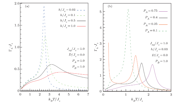
Another way to highlight the phase changes and the critical temperature through the thermal variation $e$ of the Gruneisen ratio $\Gamma_{h}$ as shown in Figs. 3(a) and 3(b) where $\Gamma_{h}$ exhibits a peak or diverges at $T_{c}$. It should be well to note that the values of $T_{c}$ determined from T-$\Gamma_{h}$ curves are close to those found by the direct calculation (Fig. 2).
Fig. 3
 New window|Download| PPT slide
Fig. 3(Color online) The normalized Gruneisen ratio as a function of normalized temperature for fixed external magnetic field ($h/Jz$=0.03) for various concentration magnetic component in sublattice $A$ (a) and for various values of external magnetic field (b).
It is seen also that the effect of dilution on $\Gamma_{h}$ ratio occurs through some peaks, which are shifted toward lower temperature while the concentration of magnetic atoms decreases, in the same time these observed peaks around transition point are shifted and broadened toward higher temperature with increasing the external magnetic field.
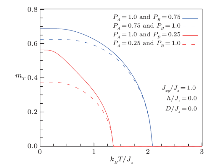
In Fig. 4, we have outlined the concentration influence of the magnetic entities, of respective spins 1/2 and 1, on the spontaneous magnetization ($h$=0) for $J_{xy}/J_{z}$=1 and $D$=0, ie isotropic Heisenberg system. We note that except the magnitude of the magnetization, its general behavior is preserved even if alternating the concentrations $p_{A}$ and $p_{B}$.
Fig. 4
 New window|Download| PPT slide
Fig. 4(Color online) Thermal dependence of the total magnetization for selected values of concentrations $p_A$ and $p_B$ of the two magnetic species.
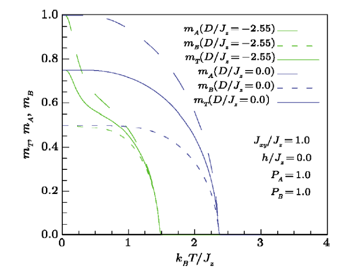
In Fig. 5, we have reported the thermal variation of the spontaneous magnetizations (per spin) corresponding of the sublattice $A$ and $B$ as well as the global magnetization of the system in the absence of dilution ($p_{A}$ = $p_{B}$=1) in two significant cases: in the absence of crystalline anisotropy ($D/J_{z}$ = 0) and the case of strong negative anisotropy ($D/J_{z}$ = $-$2.55). We note that when the anisotropy is negative and important, the magnetization of the sublattice $A$ with spin 1 is strongly influenced by this anisotropy, which favors spin confinement in the ($x, y$) plane and thus leads to a remarkable reduction of the critical temperature.
Fig. 5
 New window|Download| PPT slide
Fig. 5(Color online) Thermal dependencies of the sublattice magnetizations $m_A$, $m_B$ and total magnetization per site $m_T$ for the mixed spin-1 and spin-1/2, for $D/Jz$ = —2.55 and 0.0.
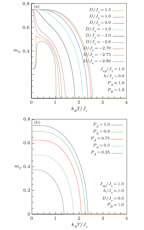
In Fig. 6, we conjointly analyze the effect of the concentration of spin-1 species $A$ and the effect of single-ion anisotropy on the spontaneous magnetization of the system. We note that the critical temperature as well as the spontaneous magnetization at 0 K increase with the concentration $p_{A}$ (a), whereas the ionic anisotropy strength impact seriously both the M (0) magnitude, the $T_c$ value as well as the shape of spontaneous magnetization curves (b), in particular, for negative anisotropy cases. Thus, the thermal variation of the magnetization goes from a behavior of type-Q for $D>$ 0 to type-M ($D/J_{z}$ =—2.6) or type-P ($D/J_{z}$ =—2.8) in the Néel Classification.[33] In fact, when $D$ is negative and sufficiently strong, the spins of the sublattice $A$ are substantially polarized in opposite directions to those of the sublattice $B$, and since the spins $S_{A}$ and $S_{B}$ are quite different, this produces a ferrimagnetic regime. It should be emphasized that our findings are similar to results for the mixed spin-1 and spin-1/2 ferrimagnet on the simple cubic lattice obtained by the earlier mean-field theory,[34] as well as those obtained by the cluster variation method[35] or those established by Monte Carlo simulation.[36]
Fig. 6
 New window|Download| PPT slide
Fig. 6(Color online) Thermal dependencies of the total magnetization per site for different values of single-ion anisotropy $D/J_z$ (a) and a range of site concentration 0.25$\leq p_A\leq $1.0 (b).
3.2 Magnetocaloric Responses
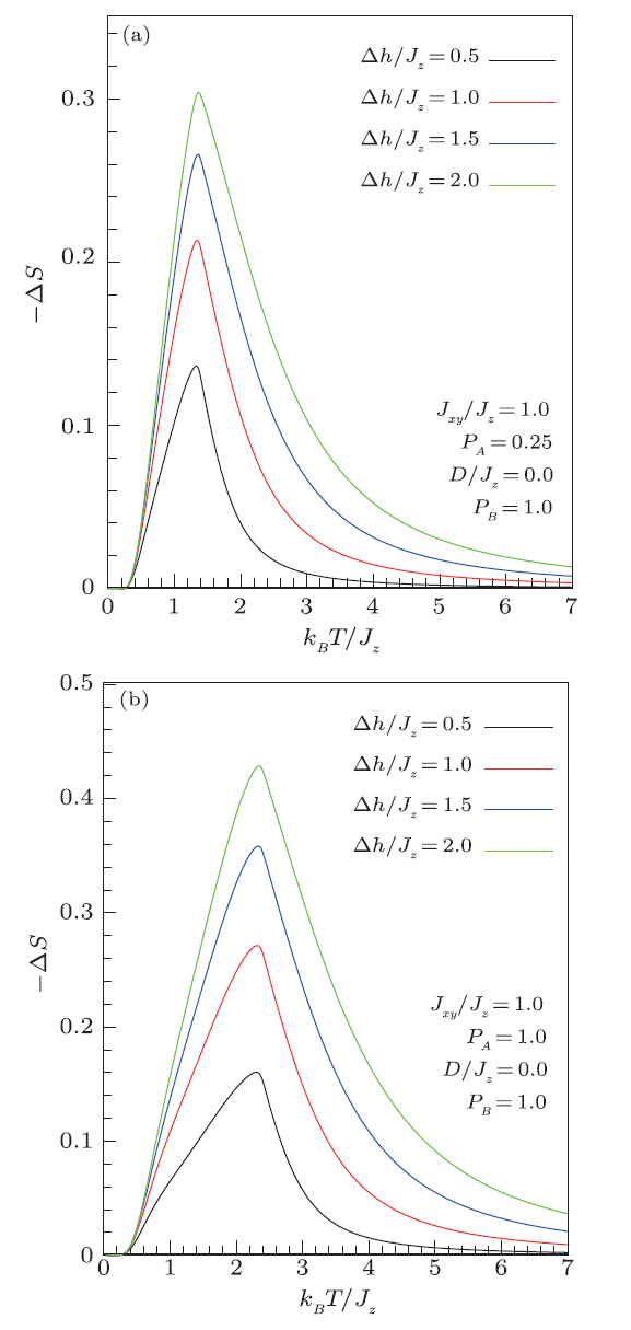
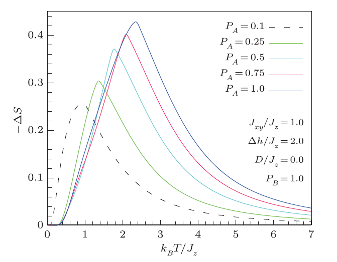
In the current subsection, we aim to elucidate the influence of various considered intrinsic parameters on the magnetocaloric responses of the system.Figure 7 depicts the computed isothermal magnetic entropy change (for $J_{z}/J_{xy}$= 1, $D/J_{z}$=0) versus temperature upon different external magnetic fields for $p_{A}$ =0.25 (a) and $p_{A}$=1.0 (b). It should be stressed that for higher concentrations of spin entities $S_{A}$, $-\Delta{}S$ becomes larger and undergoes a higher maximum (see Fig. 8), which would lead to noticeable improvements in the magnetocaloric effects of the system.
Fig. 7
 New window|Download| PPT slide
Fig. 7(Color online) Temperature dependence of the entropy change in mixed system upon a magnetic field change when the concentration of magnetic atoms is $p_A$=0.25 (a) or $p_A$= 1.0 (b), when the sublattice $B$ is not diluted ($p_B$=1).
Fig. 8
 New window|Download| PPT slide
Fig. 8(Color online) Temperature dependence of the entropy change in mixed system upon a magnetic field change ($\Delta{}h/J_z$=2) for different values of $p_A$.
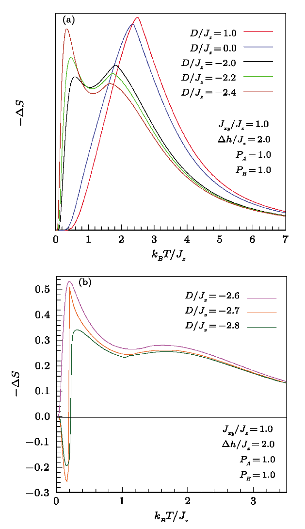
The influence of single-ion anisotropy $D$ on the entropy change illustrated in Figs. 9(a) and 9(b). For the positive values of $D$ enhancing ferromagnetic behaviors, $-\Delta{}S$ enlarges hugely with $D$, whereas for the negative values of $D$ we observe a doubling of the $-\Delta{}S$ maximum and its widening (see for example the curve labeled $D/J_{z}=-$2.2 in Fig. 9(a). A similar effect has been observed in composites,[37] magnetic multilayer with antiferromagnetic interlayers[38] and other materials.[39] Finally note that for higher negative $D$, the system becomes ferrimagnetic (Fig. 9(b)).
Fig. 9
 New window|Download| PPT slide
Fig. 9(Color online) Thermal variation of the entropy change in mixed binary system upon a magnetic field change ($\Delta{}h/J_z$=2) for different values the single-ion anisotropy constant $D$.
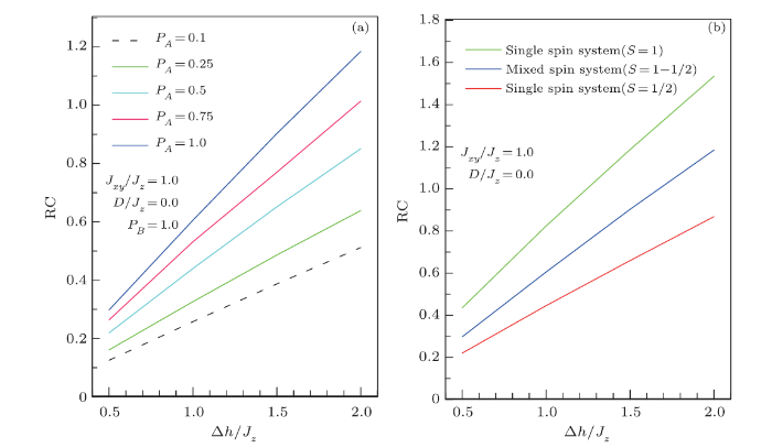
To quantify the performance of the system in refrigeration (Ericsson) cycle,[40] we report on Fig. 10 the RC behavior, which appears to change almost linearly with the intensity of external field for different concentrations of $S_{A}$ (a) and for three extreme cases (b). It is clear from the two sets of curves that the RC improvement requires a high spin material with strong ferromagnetic couplings.
Fig. 10
 New window|Download| PPT slide
Fig. 10(Color online) Field dependence of RC parameter in mixed binary system upon a magnetic field change for different values the $p_A$ concentration (a) and for three cases of spin magnitude (b).
4 Conclusion
In this paper, we have investigated the effects of dilution, exchange coupling and single-ion anisotropy on the phase diagram and the MCE of the diluted mixed spin-1 and spin-1/2 anisotropic quantum Heisenberg model on simple cubic lattice. We have established that the spin strength, the concentration of the magnetic species and the ionic anisotropy are determining factors for the magnetic behavior of the system and govern its magnetocaloric properties.This study would guide experimental researchers to conceive suitable materials with improved performance for magnetic refrigeration.
Reference By original order
By published year
By cited within times
By Impact factor
[Cited within: 1]
[Cited within: 1]
[Cited within: 1]
[Cited within: 1]
[Cited within: 2]
[Cited within: 1]
[Cited within: 1]
[Cited within: 1]
[Cited within: 1]
[Cited within: 1]
[Cited within: 1]
[Cited within: 1]
[Cited within: 1]
[Cited within: 3]
[Cited within: 2]
[Cited within: 1]
[Cited within: 1]
[Cited within: 1]
[Cited within: 1]
[Cited within: 1]
[Cited within: 1]
[Cited within: 1]
URL [Cited within: 1]
[Cited within: 1]
[Cited within: 1]
[Cited within: 1]
[Cited within: 1]
[Cited within: 1]
[Cited within: 1]
[Cited within: 1]
[Cited within: 1]
[Cited within: 1]
[Cited within: 1]
