Yu Sun^,1,2, Gaoke Hu³, Yongwen Zhang⁴, Bo Lu⁵, Zhenghui Lu⁶, Jingfang Fan⁷, Xiaoteng Li⁸, Qimin Deng⁹, Xiaosong Chen^,7,∗1Institute of Theoretical Physics, Key Laboratory of Theoretical Physics, Chinese Academy of Sciences, PO Box 2735, Beijing 100190, China
²School of Physical Sciences, University of Chinese Academy of Science, No. 19A Yuquan Road, Beijing 100049, China
³Beijing Computational Science Research Center, Beijing 100193, China
⁴Data Science Research Center, Kunming University of Science and Technology, Kunming 650500, China
⁵Laboratory for Climate Studies, National Climate Center, China Meteorological Administration, Beijing 100081, China
⁶CAS Key Laboratory of Regional Climate Environment for Temperate East Asia, Institute of Atmospheric Physics, Chinese Academy of Sciences, Beijing 100029, China
⁷School of Systems Science, Beijing Normal University, Beijing 100875, China
⁸Harvest Fund Management, Beijing 100021, China
⁹Lab for Climate and Ocean-Atmosphere Studies, Dept. of Atmospheric and Oceanic Sciences, School of Physics, Peking University, Beijing, 100871, China

First author contact: ∗Author to whom any correspondence should be addressed.
Received:2021-01-21Revised:2021-03-23Accepted:2021-03-24Online:2021-05-06


Abstract
Emergence refers to the existence or formation of collective behaviors in complex systems. Here, we develop a theoretical framework based on the eigen microstate theory to analyze the emerging phenomena and dynamic evolution of complex system. In this framework, the statistical ensemble composed of M microstates of a complex system with N agents is defined by the normalized N × M matrix A, whose columns represent microstates and order of row is consist with the time. The ensemble matrix A can be decomposed as ${\boldsymbol{A}}={\sum }_{I=1}^{r}{\sigma }_{I}{{\boldsymbol{U}}}_{I}\otimes {{\boldsymbol{V}}}_{I}$, where $r={\rm{\min }}(N,M)$, eigenvalue σ_I behaves as the probability amplitude of the eigen microstate U_I so that ${\sum }_{I=1}^{r}{\sigma }_{I}^{2}=1$ and U_I evolves following V_I. In a disorder complex system, there is no dominant eigenvalue and eigen microstate. When a probability amplitude σ_I becomes finite in the thermodynamic limit, there is a condensation of the eigen microstate U_I in analogy to the Bose-Einstein condensation of Bose gases. This indicates the emergence of U_I and a phase transition in complex system. Our framework has been applied successfully to equilibrium three-dimensional Ising model, climate system and stock markets. We anticipate that our eigen microstate method can be used to study non-equilibrium complex systems with unknown order-parameters, such as phase transitions of collective motion and tipping points in climate systems and ecosystems.
Keywords： complex system;phase transition;critical phenomena;Earth system;statistical ensemble;eigen microstate;dynamic evolution;econophysics


PDF (0KB)MetadataMetricsRelated articlesExportEndNote|Ris|BibtexFavorite
Cite this article
Yu Sun, Gaoke Hu, Yongwen Zhang, Bo Lu, Zhenghui Lu, Jingfang Fan, Xiaoteng Li, Qimin Deng, Xiaosong Chen. Eigen microstates and their evolutions in complex systems. Communications in Theoretical Physics, 2021, 73(6): 065603- doi:10.1088/1572-9494/abf127

1. Introduction

Statistical physics is a field of physics that studies the macroscopic behaviors of large collection of interacting objects based on their microscopic properties. Traditionally, these objects can be atoms, molecules, magnetic spins, electrons, quanta such as photons and phonons, et al. In recent decades, statistical physics has been extended to study complex systems consisting of many other types of interacting objects, such as individuals in populations, species in an ecosystem, agents in a market, computers in a network, et al. The studies of collective phenomena emerging from the interactions between individuals of social system are reviewed recently [1]. With the use of ideals and mathematical methods developed in statistical physics to economic systems, a new interdisciplinary research field is established and called econophysics [2]. The criticality and dynamical scaling of statistical physics are found in living systems also [3].

The concept of statistical ensemble was introduced by Gibbs [4] in 1902 and serves as a starting point of statistical physics. At a certain time, the states of all individuals in a system can be represented by a point in the high dimensional phase space, which is called a microstate of the system. All microstates under a certain macroscopic condition constitute an ensemble of the system. The ensemble can be described by the probability density of microstate. The macroscopic properties of the system can be obtained by averaging over all microstates.

Three important ensembles were defined by Gibbs [4] under different thermodynamic conditions. They are the micro-canonical ensemble, the canonical ensemble, and the grand canonical ensemble, respectively. The probability density of microstate in an ensemble is known for thermodynamic systems in equilibrium. All microstates in a micro-canonical ensemble have the same probability. In the canonical ensemble with temperature T, the probability density of a microstate with energy E is proportional to $\exp \left(-E/{k}_{{\rm{B}}}T\right)$, where k_B is the Boltzmann constant. For the grand canonical ensemble with temperature T and chemical potential $\mu$, the probability of a microstate with energy E and particle number N is proportional to $\exp \left(-E/{k}_{{\rm{B}}}T+\mu N/{k}_{{\rm{B}}}T\right)$. In principle, the thermodynamic properties of equilibrium systems can be calculated from these probability densities of microstate.

A large number of complex systems that need to be studied at present are generally not in equilibrium. Their probability densities of microstate are unknown. This is a huge challenge for studying the macroscopic properties of complex systems from the interaction between individuals. As pointed out recently in the commentary [5], the complexity at mesoscales of different levels arises from collective effects. The studies at mesoscales could be an essential step to tackle complex systems. We have proposed a method [6] to study the eigen microstates of complex system, which capture structures of mesoscales. According this method, we can get microstates and the ensemble of a complex system from its experimental investigations or computer simulations. In the original ensemble, microstates are not independent each other. Using the eigenvectors of the correlation matrix between microstates, eigen microstates can be obtained. In the ensemble composed of eigen microstates, there is no correlation between eigen microstates, which have weights proportional to the square of eigenvalue. For a complex systems without localization of microstate, the weight of an eigen microstate approaches zero in the thermodynamic limit. When the weight of an eigen microstate has a finite limit, there is then a condensation of the eigen microstate in the ensemble. This is similar to the Bose-Einstein condensation of Bose gas. The condensation of eigen microstate corresponds to a phase transition with new phase described by the eigen microstate and the eigenvalue as its order parameter. In the studies of phase transitions until now [46], order-parameter is served as the starting point. But the order-parameters of many complex systems are unknown at first. This bottleneck can be overcome by our eigen microstate method.

Complex systems in non-equilibrium are always in the course of evolution. We should study not only eigen microstates but also their evolution. Here we present the method to characterize the evolution of eigen microstate in section 2. The condensation of eigen microstate and its relation to a phase transition are discussed in section 2.2. To demonstrate the effectiveness of our method, we have studied the eigen microstates and their evolutions of the equilibrium three-dimensional Ising model, the global temperature fluctuation of Earth, and the price fluctuation in the stock markets of Chinese mainland. Finally, we make some conclusions in section 5.

2. Eigen microstates and their evolutions

For a complex system composed of N agents, we can obtain the states of the agents from experimental measurements or computer simulations. Using the states at times t = 1, 2, ⋯ , M in sequence, we can get the state series S_i(t) of agents i = 1, 2, …, N.

The average state of an agent i is
(1)$\begin{eqnarray}\langle {S}_{i}\rangle =\displaystyle \frac{1}{M}\displaystyle \sum _{t=1}^{M}{S}_{i}(t).\end{eqnarray}$


At a certain time t, the agent i has a fluctuation
(2)$\begin{eqnarray}\delta {S}_{i}(t)={S}_{i}(t)-\langle {S}_{i}\rangle .\end{eqnarray}$
We define a microstate with fluctuations of all agents, which is represented by an N-dimensional vector [6]
(3)$\begin{eqnarray}\delta {\boldsymbol{S}}(t)=\left[\begin{array}{c}\delta {S}_{1}(t)\\ \delta {S}_{2}(t)\\ \vdots \\ \delta {S}_{N}(t)\end{array}\right].\end{eqnarray}$


With the M microstates, we can compose a statistical ensemble of the complex system. This ensemble is described by an N × M matrix A with elements
(4)$\begin{eqnarray}{A}_{{it}}=\displaystyle \frac{\delta {S}_{i}(t)}{\sqrt{{C}_{0}}},\end{eqnarray}$
where ${C}_{0}={\sum }_{t=1}^{M}{\sum }_{i=1}^{N}\delta {S}_{i}^{2}(t)$. The column order of A is in accord with the evolution of microstate.

As in [6], the correlation between the microstates at t and $t^{\prime} $ is defined by their vector product
(5)$\begin{eqnarray}{C}_{{tt}^{\prime} }=\delta {\boldsymbol{S}}{\left(t\right)}^{{\rm{T}}}\cdot \delta {\boldsymbol{S}}(t^{\prime} )=\displaystyle \sum _{i=1}^{N}\delta {S}_{i}(t)\delta {S}_{i}(t^{\prime} ).\end{eqnarray}$
With ${C}_{{tt}^{\prime} }$ as its elements, we can get an M × M correlation matrix of microstate
(6)$\begin{eqnarray}{\boldsymbol{C}}={C}_{0}{{\boldsymbol{A}}}^{{\rm{T}}}\cdot {\boldsymbol{A}}\,\end{eqnarray}$
whose trace ${\rm{Tr}}{\boldsymbol{C}}={\sum }_{t=1}^{M}{C}_{{tt}}={C}_{0}$.

The statistical ensemble can also be considered as an ensemble of dynamic microstates of agent, which are described by M-dimensional vectors
(7)$\begin{eqnarray}\delta {{\boldsymbol{S}}}_{i}=\left[\delta {S}_{i}(1),\delta {S}_{i}(2),\cdots ,\delta {S}_{i}(M)\right],\end{eqnarray}$
where i = 1, 2, ⋯ ,N.

In addition, we consider here the correlation between the dynamic microstates δS_i and δS_j
(8)$\begin{eqnarray}{K}_{{ij}}=\delta {{\boldsymbol{S}}}_{i}\cdot \delta {{\boldsymbol{S}}}_{j}^{{\rm{T}}}=\displaystyle \sum _{t=1}^{M}\delta {S}_{i}(t)\delta {S}_{j}(t).\end{eqnarray}$
With K_ij as its elements, we can get an N × N correlation matrix of dynamic microstate
(9)$\begin{eqnarray}{\boldsymbol{K}}={C}_{0}{\boldsymbol{A}}\cdot {{\boldsymbol{A}}}^{{\rm{T}}},\end{eqnarray}$
whose trace ${\rm{Tr}}({\boldsymbol{K}})={\sum }_{i=1}^{N}{K}_{{ii}}={C}_{0}$.

The correlation matrix C has M eigenvectors V_J of J = 1, 2, ⋯ , M. With them we can compose an M × M unitary matrix
(10)$\begin{eqnarray}{\boldsymbol{V}}=\left[{{\boldsymbol{V}}}_{1}{{\boldsymbol{V}}}_{2}...{{\boldsymbol{V}}}_{M}\right].\end{eqnarray}$


The correlation matrix K has N eigenvectors U_I of I = 1, 2, ⋯ , N. From these eigenvectors, we can obtain an N × N unitary matrix
(11)$\begin{eqnarray}{\boldsymbol{U}}=\left[{{\boldsymbol{U}}}_{1}{{\boldsymbol{U}}}_{2}...{{\boldsymbol{U}}}_{N}\right].\end{eqnarray}$


According to the singular value decomposition (SVD) [7], the ensemble matrix A can be factorized as
(12)$\begin{eqnarray}{\boldsymbol{A}}={\boldsymbol{U}}\cdot {\boldsymbol{\Sigma }}\cdot {{\boldsymbol{V}}}^{{\rm{T}}},\end{eqnarray}$
where Σ is an N × M diagonal matrix with elements
(13)$\begin{eqnarray}\begin{array}{c}{{\rm{\Sigma }}}_{IJ}=\left\{\begin{array}{ll}{\sigma }_{I}, & {\rm{f}}{\rm{o}}{\rm{r}}\,I=J\leqslant r,\\ 0, & {\rm{f}}{\rm{o}}{\rm{r}}\,{\rm{o}}{\rm{t}}{\rm{h}}{\rm{e}}{\rm{r}}{\rm{w}}{\rm{i}}{\rm{s}}{\rm{e}},\end{array}\right.\end{array}\end{eqnarray}$
where $r={\rm{\min }}(N,M)$.

Furthermore, we can rewrite the ensemble matrix A as
(14)$\begin{eqnarray}{\boldsymbol{A}}=\displaystyle \sum _{I=1}^{r}{\sigma }_{I}{{\boldsymbol{A}}}_{I}^{e},\end{eqnarray}$
where ${{\boldsymbol{A}}}_{I}^{e}\equiv {{\boldsymbol{U}}}_{I}\otimes {{\boldsymbol{V}}}_{I}$ is an N × M matrix with elements ${\left({{\boldsymbol{A}}}_{I}^{e}\right)}_{{it}}={U}_{{iI}}{V}_{{tI}}$. We call the ensemble defined by ${{\boldsymbol{A}}}_{I}^{e}$ an eigen ensemble of system. From statistical ensemble, we can obtain not only eigen microstate U_I, which has been introduced in [6], but also their evolution with time V_I.

From ${\rm{Tr}}{\boldsymbol{C}}={C}_{0}$ or ${\rm{Tr}}{\boldsymbol{K}}={C}_{0}$, we have the relation
(15)$\begin{eqnarray}\displaystyle \sum _{I=1}^{r}{\sigma }_{I}^{2}=1.\end{eqnarray}$


Therefore, we consider σ_I as the probability amplitude and ${w}_{I}={\sigma }_{I}^{2}$ as the probability of the eigen ensemble ${{\boldsymbol{A}}}_{I}^{e}$ in the statistical ensemble A. This is analogous to quantum mechanics, where a wave function can be written in terms of eigen functions. The square of the absolute value of expansion coefficient is the probability of the corresponding eigen microstate.

Using M eigenvectors of C, we can obtain eigen microstates [6]
(16)$\begin{eqnarray}\delta {{\boldsymbol{S}}}^{e}(I)=\displaystyle \sum _{t=1}^{M}\delta {\boldsymbol{S}}(t){V}_{{tI}},\end{eqnarray}$
whose components
(17)$\begin{eqnarray}\delta {S}_{i}^{e}(I)=\displaystyle \sum _{t=1}^{M}{A}_{{it}}{V}_{{tI}}={\left({\boldsymbol{A}}\cdot {\boldsymbol{V}}\right)}_{{iI}}={\left({\boldsymbol{U}}\cdot {\boldsymbol{\Sigma }}\right)}_{{iI}}.\end{eqnarray}$
Therefore, we have
(18)$\begin{eqnarray}\begin{array}{c}\delta {{\boldsymbol{S}}}^{e}(I)=\left\{\begin{array}{ll}{\sigma }_{I}{{\boldsymbol{U}}}_{I}, & {\rm{f}}{\rm{o}}{\rm{r}}\,I\leqslant r,\\ 0, & {\rm{f}}{\rm{o}}{\rm{r}}\,{\rm{o}}{\rm{t}}{\rm{h}}{\rm{e}}{\rm{r}}{\rm{w}}{\rm{i}}{\rm{s}}{\rm{e}}.\end{array}\right.\end{array}\end{eqnarray}$
U_I is the normalized eigen microstate. Between different eigen microstates, there is no correlation.

We can express original microstates by eigen microstates as
(19)$\begin{eqnarray}\delta {\boldsymbol{S}}(t)=\displaystyle \sum _{I=1}^{M}{V}_{{tI}}\delta {{\boldsymbol{S}}}^{e}(I)=\displaystyle \sum _{I=1}^{r}{\sigma }_{I}{V}_{{tI}}{{\boldsymbol{U}}}_{I}.\end{eqnarray}$


Using N eigenvectors of K, we can get eigen dynamic microstates [8]
(20)$\begin{eqnarray}\delta {{\boldsymbol{S}}}_{I}^{e}=\displaystyle \sum _{j=1}^{N}\delta {{\boldsymbol{S}}}_{j}{U}_{{jI}},\end{eqnarray}$
whose components
(21)$\begin{eqnarray}\delta {S}_{I}^{e}(t)=\displaystyle \sum _{j=1}^{N}{A}_{{jt}}{U}_{{jI}}={\left({{\boldsymbol{U}}}^{{\rm{T}}}\cdot {\boldsymbol{A}}\right)}_{{It}}={\left({\boldsymbol{\Sigma }}\cdot {{\boldsymbol{V}}}^{{\rm{T}}}\right)}_{{It}}.\end{eqnarray}$
Further, we get
(22)$\begin{eqnarray}\begin{array}{c}\delta {{\boldsymbol{S}}}_{I}^{e}(t)=\left\{\begin{array}{ll}{\sigma }_{I}{{\boldsymbol{V}}}_{I}^{{\rm{T}}}, & {\rm{f}}{\rm{o}}{\rm{r}}\,I\leqslant r,\\ 0, & {\rm{f}}{\rm{o}}{\rm{r}}\,{\rm{o}}{\rm{t}}{\rm{h}}{\rm{e}}{\rm{r}}{\rm{w}}{\rm{i}}{\rm{s}}{\rm{e}},\end{array}\right.\end{array}\end{eqnarray}$
where ${{\boldsymbol{V}}}_{I}^{{\rm{T}}}$ is the normalized eigen dynamic microstate. Different eigen dynamic microstates have no correlation each other and are independent.

2.1. Fourier spectrum analysis of eigen microstate evolution

The time evolution of the Ith eigen microstate is described by ${{\boldsymbol{V}}}_{I}^{{\rm{T}}}=\left[{V}_{1I},{V}_{2I},\cdots ,{V}_{{MI}}\right]$. To get more information about the evolution of eigen microstate, we expand V_tI by a Fourier series
(23)$\begin{eqnarray}{V}_{{tI}}=\displaystyle \sum _{n=0}^{M-1}{b}_{{nI}}{{\rm{e}}}^{{\rm{i}}\tfrac{2\pi }{M}{nt}},\,\end{eqnarray}$
where the Fourier coefficients are
(24)$\begin{eqnarray}{b}_{{nI}}=\displaystyle \frac{1}{M}\displaystyle \sum _{t=0}^{M-1}{V}_{{tI}}{{\rm{e}}}^{-{\rm{i}}\tfrac{2\pi }{M}{nt}}.\end{eqnarray}$


To characterize the proportion of different frequences, we introduce the Fourier power spectrum density
(25)$\begin{eqnarray}{I}_{n}=\displaystyle \frac{| {b}_{n}^{I}{| }^{2}}{{\displaystyle \sum }_{n=0}^{M-1}| {b}_{n}^{I}{| }^{2}},\end{eqnarray}$
which will be shown with respect to its period T_n = M/n.

2.2. Condensation of eigen microstate and phase transition

In a statistical ensemble without localization of microstate, the weights of all eigen microstates are of the same order. In the limits M → ∞ and N → ∞ , all probability amplitudes σ_I → 0. In this case, the system is in a random and disorder state.

If a probability amplitude σ_I becomes dominant so that it has a finite limit at M → ∞ and N → ∞ , there is a condensation of eigen microstate ${{\boldsymbol{A}}}_{I}^{e}$ in the statistical ensemble. This is similar to the Bose-Einstein condensation of Bose gases, where a finite proportion of infinite bosons share the lowest quantum state. This condensation indicates the appearance of a new phase in the Bose gas and there is a phase transition. The condensation of an eigen microstate manifests that a finite proportion of infinite eigen microstates share this eigen microstate. A new phase appears in the system. The new phase is characterized by the eigen microstate U_I. The evolution of new phase is described by V_I.

If σ_I increases to finite continuously, the complex system experiences a continuous phase transition. With a jump of σ_I at transition point, there is a discontinuous phase transition.

For system with finite N, the limit of σ_I for M → ∞ can be obtained with large enough M [6]. For a continuous phase transition, the distance from critical point T_c is defined as t = (T − T_c)/T_c. In the asymptotic region with ∣t∣ ≪ 1, we propose the finite-size form of σ_I [6] as
(26)$\begin{eqnarray}{\sigma }_{I}(T,N)={N}^{-\beta /d\nu }{f}_{I}({{tN}}^{1/d\nu }),\end{eqnarray}$
where $\beta$ is the critical exponent of order parameter and ν is the critical exponent of correlation length.

Correspondingly, the ratio σ₂/σ₁ follows the finite-size scaling form [9]
(27)$\begin{eqnarray}{\sigma }_{2}/{\sigma }_{1}=R({{tN}}^{1/d\nu }),\end{eqnarray}$
which has a fixed point at critical point t = 0.

In the bulk limit N → ∞ , we obtain the bulk order parameter
(28)$\begin{eqnarray}{\sigma }_{1}(T,\infty )=\left\{\begin{array}{ll}{a}_{1}\,{\left(-t\right)}^{\beta }, & \mathrm{for}\ t\leqslant 0,\\ 0, & \mathrm{for}\ t\gt 0.\end{array}\right.\end{eqnarray}$


The eigen microstates and their condensation in one- and two-dimensional equilibrium Ising models have been investigated [8, 6]. Near and below critical point, the largest eigen microstate (EM1) U₁ becomes a cluster with spins of the same orientation. For the second largest eigen microstate (EM2) U₂, there are two clusters which have opposite orientation. The finite-size scaling of probability amplitude in equation (26) has been confirmed by Monte Carlo simulation data of one- and two-dimensional Ising models [6].

In the next section, we will study the condensation of eigen microstate and their evolution in equilibrium three-dimensional Ising model by Monte Carlo simulations. To demonstrate that our method presented above can be used to general complex systems, the eigen microstates of the Earth system and stock markets will be explored in section 4.

3. Application to equilibrium system

We consider a three-dimensional Ising model with square geometry and periodic boundary conditions. The Hamiltonian of N = L × L × L spins is
(29)$\begin{eqnarray}H=-J\displaystyle \sum _{\langle i,j\rangle }^{N}{S}_{i}{S}_{j},\end{eqnarray}$
where S_i = ± 1 and ⟨i, j⟩ means a summation over all spins in the nearest neighbourhood. The model is characterized by the system size L and the reduced temperature T^* = k_BT/J. We can obtain microstates of the system using the Wolff algorithm [10], which flips a cluster of spins rather than a single spin.

In a finite Ising system, there is no symmetry breaking. Therefore ⟨S_i⟩ = 0 and δS_i(t) = S_i(t). The microstate at time t is
(30)$\begin{eqnarray}\delta {\boldsymbol{S}}(t)=\left[\begin{array}{c}\delta {S}_{1}(t)\\ \delta {S}_{2}(t)\\ \vdots \\ \delta {S}_{N}(t)\end{array}\right].\end{eqnarray}$
Using these microstates, we get the ensemble matrix A with elements
(31)$\begin{eqnarray}{A}_{{it}}=\displaystyle \frac{\delta {S}_{i}(t)}{\sqrt{{C}_{0}}},\end{eqnarray}$
where C₀ = M · N.

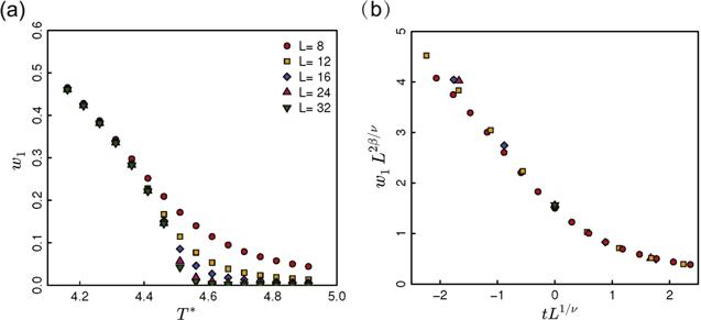
In figure 1(a), the largest probability ${w}_{1}={\sigma }_{1}^{2}$ is plotted with respect to T^*. At higher temperatures, w₁ is very small and comparable to other probabilities. With the decrease of temperature, w₁ increases faster and becomes dominant. This indicates the emergence of a new phase and there is a phase transition.

Figure 1.

New window|Download| PPT slide
Figure 1.(a) Weight w₁ of the largest eigen ensemble matrix with respect to reduced temperature T^* = k_BT/J. (b) Finite-size scaling form of w₁ with respect to tL^1/ν, where t = (T − T_c)/T_c.


The finite-size scaling form of w₁ is presented in figure 1(b). To calculate the scaling variable, the critical temperature ${T}_{c}^{* }\simeq 4.5114$ [11] and the critical exponent of correlation length ν = 0.6335 [12] are used. Our simulation data confirm the finite-size scaling form of w₁.

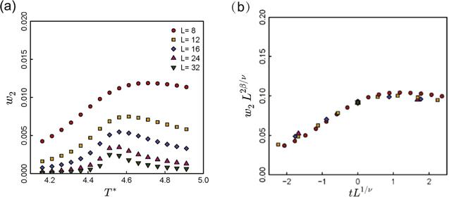
The second largest probability w₂ and its finite-size scaling form are shown in figure 2. Near the critical point ${T}_{c}^{* }$, w₂ becomes finite and its finite-size scaling form is confirmed also.

Figure 2.

New window|Download| PPT slide
Figure 2.(a) Weight w₂ with respect to reduced temperature T^* = k_BT/J. (b) Finite-size scaling form of w₂ with respect to tL^1/ν, where t = (T − T_c)/T_c.


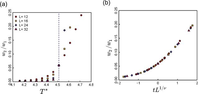
In figure 3(a), the ratio ${w}_{2}/{w}_{1}={\left({\sigma }_{2}/{\sigma }_{1}\right)}^{2}$ is plotted with respect to T^*. A fixed point is found at the critical temperature ${T}_{c}^{* }$. The finite-size scaling form of w₂/w₁ is presented in figure 3(b). The finite-size scaling form of eigenvalues has been verified completely in three-dimensional Ising model also. This is in accord with the finite-size scaling of correlation function [13].

Figure 3.

New window|Download| PPT slide
Figure 3.(a) Ratio w₂/w₁ with respect to reduced temperature T^* = k_BT/J. (b) Finite-size scaling form of w₂/w₁ with respect to tL^1/ν, where t = (T − T_c)/T_c.


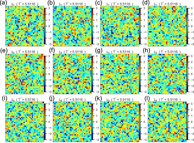
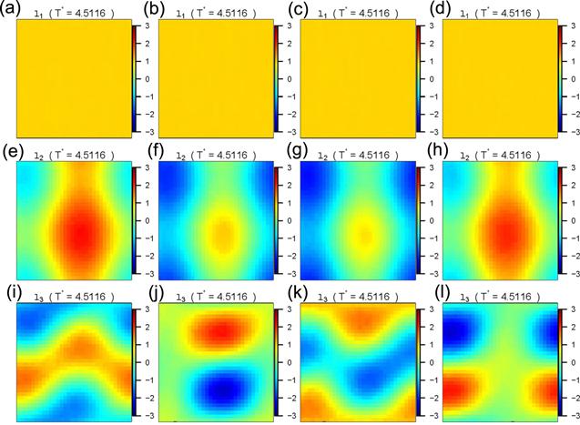
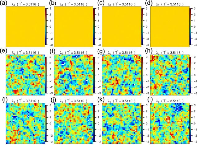
We identify the character of phase transition by studying the spatial distribution of eigen microstates U_I. For an eigen microstate in three-dimensional space, four sectional drawings with equal distance are presented. In figure 4, we show three eigen microstates U₁, U₂, and U₃ at reduced temperature T^* = 5.5116, which is above the critical temperature. The clusters of spins in these eigen microstates are of micro size and distributed randomly in space.

Figure 4.

New window|Download| PPT slide
Figure 4.Four sectional drawings with equal distance of eigen microstates U₁, U₂, and U₃ at reduced temperature T^* = 5.5116.


At temperatures near and below critical point, the largest eigen microstate (EM1) becomes a single cluster with the system size. The results are presented in figures 5 and 6. A ferromagnetic phase appears when the probability of the eigen microstate becomes finite.

Figure 5.

New window|Download| PPT slide
Figure 5.Four sectional drawings with equal distance of U₁, U₂, and U₃ at T^* = 4.5116.

Figure 6.

New window|Download| PPT slide
Figure 6.Four sectional drawings with equal distance of U₁, U₂, and U₃ at T^* = 3.5116.


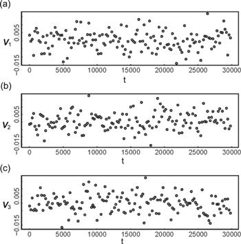
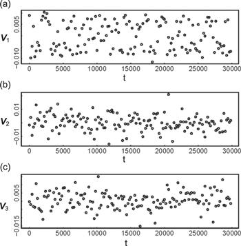
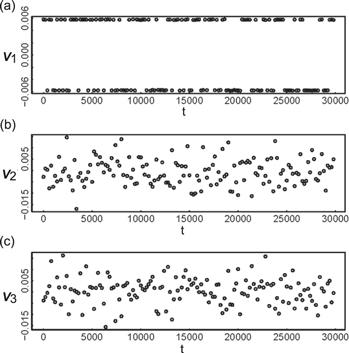
The evolutions of eigen microstates around critical point are shown in figures 7-9. In relation to the dynamics of the Wolff algorithm [10], V_tI fluctuates around zero with time t.

Figure 7.

New window|Download| PPT slide
Figure 7.Evolutions of the largest three eigen microstates at T^* = 5.5116.

Figure 8.

New window|Download| PPT slide
Figure 8.Evolutions of the largest three eigen microstates at T^* = 4.5116.

Figure 9.

New window|Download| PPT slide
Figure 9.Evolutions of the largest three eigen microstates at T^* = 3.5116.

4. Applications to non-equilibrium systems

4.1. Earth system

Because of nonlinear interactions and feedback loops between and within geosphere, atmosphere, hydrosphere, cryosphere, and biosphere, the Earth operates as a complex system. The statistical physics, that studies the behaviors of large collections of interacting objects, has been applied to the complex Earth system [14]. Until now, many concepts and methods in statistical physics such as correlation, synchronization, network and percolation theory, tipping points analysis et al have been used. Here we use the statistical ensemble, which is the foundation of statistical physics, to study complex Earth system. It is hoped that the statistical physics of complex Earth system will be established gradually.

As one of the most important climate phenomena on Earth, the El Niño and Southern Oscillation (ENSO) has been studied with network and its percolation [15, 16]. We consider here the Earth as a non-equilibrium complex system composed of many latitude-longitude grids. In this complex system, there are N = 94 × 192 = 18 048 grids with 1.9° × 1.875° latitude-longitude. Using a part of these grids, their principal modes are investigated recently [17]. Here the microstates of the Earth as a whole are studied based on daily surface air temperature (SAT) (2 m) provided by the National Centers for Environmental Prediction-National Center for Atmospheric Research (NCEP-NCAR) Reanalysis [18]. The dataset spans the time period between 01-January-1950 and 31-December-2018. Both the El Niño and the La Niña events are defined by the Oceanic Niño Index (ONI) from the National Oceanic and Atmospheric Administration. The ONI is defined as 3 month running mean of ERSST.v5 SST anomalies in the Niño 3.4 region (5°S-5°N, 170°W-120°W).

At a certain time t, the SAT at a grid i is T_i(t). The average SAT at the grid i during a time period M can be calculated as
(32)$\begin{eqnarray}\langle {T}_{i}\rangle =\displaystyle \frac{1}{M}\displaystyle \sum _{t=1}^{M}{T}_{i}(t).\end{eqnarray}$


The fluctuations of the SAT at the grid i are
(33)$\begin{eqnarray}\delta {T}_{i}(t)={T}_{i}(t)-\langle {T}_{i}\rangle ,t=1,2,\cdots ,M.\end{eqnarray}$
The root mean square deviation at the grid i is
(34)$\begin{eqnarray}{{\rm{\Delta }}}_{i}=\sqrt{\displaystyle \frac{1}{M}\displaystyle \sum _{t=1}^{M}\delta {T}_{i}{\left(t\right)}^{2}}.\end{eqnarray}$


It is better to characterize the fluctuations of SAT by
(35)$\begin{eqnarray}\delta {S}_{i}(t)=\delta {T}_{i}(t)/{{\rm{\Delta }}}_{i}.\end{eqnarray}$
We introduce the microstates of the Earth as
(36)$\begin{eqnarray}\delta {\boldsymbol{S}}(t)=\left[\begin{array}{c}\delta {S}_{1}(t)\\ \delta {S}_{2}(t)\\ \vdots \\ \delta {S}_{N}(t)\end{array}\right].\end{eqnarray}$


Using the dataset spanning from 01-January-1950 to 31-December-2018, we can get an N × M ensemble matrix A with elements
(37)$\begin{eqnarray}{A}_{{it}}=\displaystyle \frac{\delta {S}_{i}(t)}{\sqrt{{C}_{0}}},\end{eqnarray}$
where C₀ = M · N.

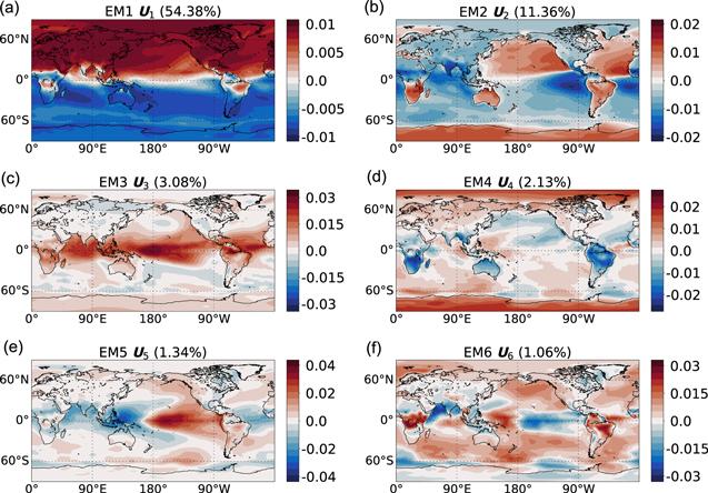
We present the eigen microstates U_I of I = 1, 2,…, 6 in figure 10. Their evolutions V_tI are shown in figure 11. In the following, we will discuss these eigen microstates in detail and their relevance to climate phenomena especially.

Figure 10.

New window|Download| PPT slide
Figure 10.Spatial distributions of the six largest eigen microstates of Earth.

Figure 11.

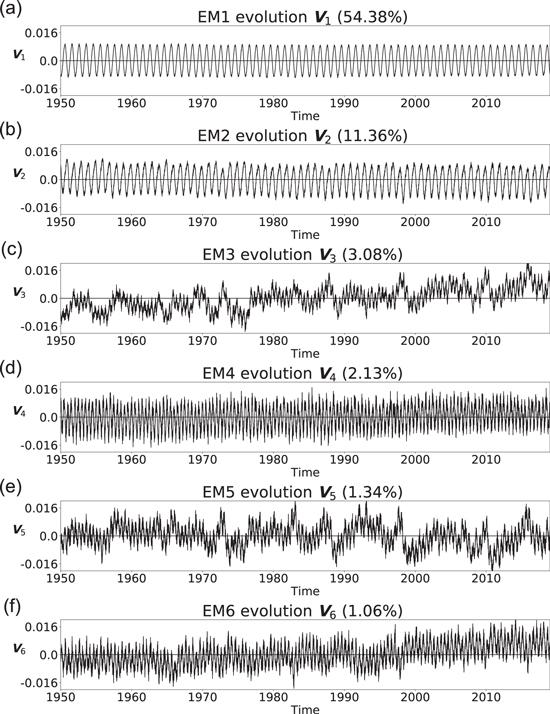New window|Download| PPT slide
Figure 11.Evolutions of the six largest eigen microstates of Earth.

4.1.1. First eigen microstate (EM1)

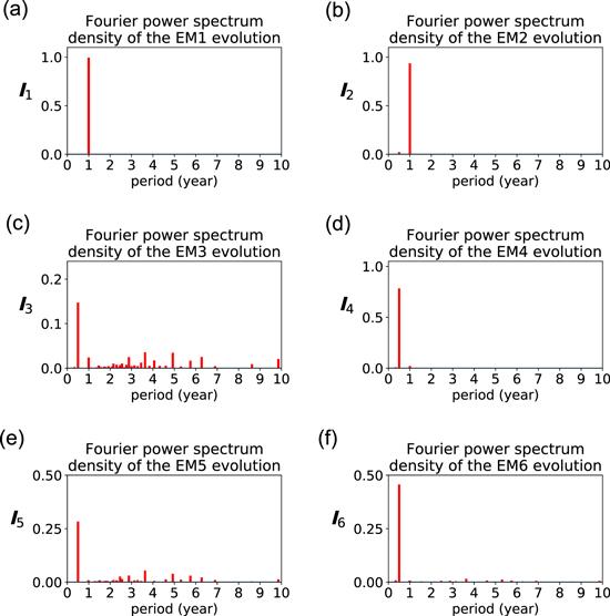
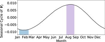
As presented in figure 10(a), EM1 reveals a classic solstitial mode and contributes 54.38% of the total variance. Its spatial pattern exhibits an inter-hemisphere contrast. This asymmetry is roughly a mirror image along the equator, although the slight shift is evident over the African, South American and Eastern Pacific sections. The spectrum analysis (figure 12(a)) of the corresponding time series (figure 11(a)) shows a robust peak at 1 year, following the annual variation of the solar zenith angle. Further results (figure 13) show that the maximum of EM1 often occurs in August and the minimum of EM1 occurs in Late January, indicating 1 month delay of air temperature after the solar forcing.

Figure 12.

New window|Download| PPT slide
Figure 12.Fourier power spectrum density of evolution for the six largest eigen microstates of Earth.

Figure 13.

New window|Download| PPT slide
Figure 13.Seasonal cycle of EM1 evolution V₁.

4.1.2. Second eigen microstate (EM2)

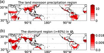
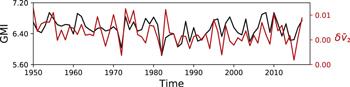
Figure 10(b) demonstrates the spatial pattern of EM2, which contributes to 11.36% of the total variance. Similar to EM1, the obvious period of 1 year is detected, implying the regular annual variation of this mode. A remarkable land-sea contrast is observed in EM2. In the southern (northern) hemisphere, the SAT warms up (cools down) faster over the continents than the oceans due to the land-sea thermal capacity difference. It should be noted that this thermal contrast in the tropical-subtropical regions drives the local monsoons over the South Asia [20], Australia [21], West Africa [22], North America [23], and South America [24]. Wang et al [19] proposed the concept of global monsoon system by considering the seasonal contrast of precipitation globally. It is interesting that the domain with the spatial absolute intensity above 40% of the maximum aboslute intensity in EM2 resembles the global monsoon area as presented in figure 14, with the spatial matching degree reaching 70%. (Since the land-sea thermal contrast is not the only cause of East Asia monsoon, the monsoon area near East Asia is not very matched [25]). We further compare the difference between summer and winter averages of V₂ with the global monsoon index (figure 15). Again, a significant correlation with R = 0.52 is obtained. The above evidences reveal that EM2 represents the land-sea contrasts of SAT which is regarded as the primary driver for monsoon.

Figure 14.

New window|Download| PPT slide
Figure 14.(a) The global monsoon area derived by Wang et al [19]. (b) The domain with the spatial absolute intensity above 40% of the maximum absolute intensity in U₂.

Figure 15.

New window|Download| PPT slide
Figure 15.(a) The GMI calculated by Wang et al [19]. (b) The difference between summer and winter averages of V₂.

4.1.3. Third eigen microstate (EM3)

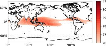
Figure 10(c) demonstrates the spatial pattern of EM3, which accounts for 3.08% of the total variance. It is featured as the climate fluctuation within the tropics. Specifically, the pronounced variations are observed over the tropical Indian Ocean, tropical Pacific Ocean and northern tropical Atlantic Ocean. As shown in figure 16, This pattern is anchored by the sea surface temperature (SST). For example, the climatology SST stays north of the equator over the Atlantic and eastern Pacific Oceans due to the wind-evaporation-SST loop feedback [26], which is well captured by the SAT pattern in EM3 (figure 10(c)). Given the fact that the tropical convection is largely coupled with the local SST, EM3 pattern is also able to reveal the tropical rainfall. For example, the intertropical convergence zone north of equator over the eastern Pacfic and Atlantic Oceans [27], as well as the wide South Pacific convergence zone [28]; also see in figure 17), are represented by EM3. The spectrum of EM3 is shown in figure 12(c). The periods of both 0.5 year and 1 year are evident. The 0.5 year period of EM3 follows the maximum solar forcing due to the Sun crossing the equator twice a year, which is evident over the Indian Ocean. Meanwhile, due to the surface wind adjustment [29], the SAT and SST in the equatorial eastern Pacific and Atlantic exhibit a distinct annual cycle despite of the occurrences of the two equinoxes, which explains the 1 year period of EM3. Figure 11(c) shows the time series of EM3. A robust upward trend is evident, implying the potential impact of global warming on the tropical SST and convective precipitation. It is interesting that a tipping point in mid-1970s is detected by EM3. This is consistent with the well-known 1976-1977 climate shift [30].

Figure 16.

New window|Download| PPT slide
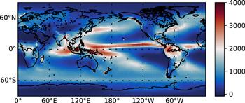
Figure 16.Annual mean sea surface temperature (SST) pattern during 1950-2018. Note that the SST below 26C is removed for clarity.

Figure 17.

New window|Download| PPT slide
Figure 17.Annual mean precipitation pattern during 1979-2018.

4.1.4. Fourth eigen microstate (EM4)

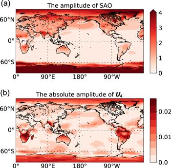
Figure 10(d) shows the spatial pattern of EM4, which explains 2.13% of the total variance. As seen in figure 10(d), the distribution of significant temperature anomaly is mainly located in the tropics and high latitudes. The EM4 evolution series (figure 11(d)) is dominated by semiannual signal as the power spectrum showing (figure 12(d)). In meteorology, this semiannual signal is called semiannual oscillation (SAO), which is component of the annual cycle of a variable that consists of a sinusoidal oscillation with a period of six months [31]. Strong semiannual signals in thermal and momentum fields of the troposphere are found in both the Tropics and in Southern Hemisphere middle and high latitudes. The SAO is detectable as a significant contribution of the second harmonic to the annual march of temperature, SAT, wind speed et al [32-35]; here, we applied a harmonic analysis method called nonlinear mode decomposition to extract its second harmonic wave and showed its amplitude as seen in the figure 18(a), which is highly consistent with the results of figure 18(b), especially in Antarctic region. Previous studies have pointed out that the mechanism of SAO in Antarctic is mainly attributed to different annual cycles of temperature in the mid-latitude ocean and Antarctic regions with the complex thermodynamics and dynamics of the ocean-atmosphere system [36-38].

Figure 18.

New window|Download| PPT slide
Figure 18.(a) The amplitude of the semiannual oscillation (SAO). (b) The absolute amplitude of U₄.

4.1.5. Fifth eigen microstate (EM5)

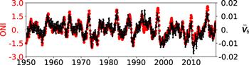
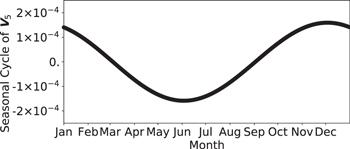
The spatial pattern of EM5 is given in figure 10(e), accounting for 1.34% of the total variance. The most remarkable feature is evident over the tropical Pacific Ocean, with the warming over the central to eastern Pacific and cooling over the western Pacific. This pattern resembles the ENSO, which is the strongest climate fluctuation at interannual time scale [39]. Spectrum analysis is conducted (figure 12(e)). Other than the semi-annual cycle, the broad spectrum is evident at interannual time scale from 2 to 7 years in EM5, which is consistent with ENSO spectrum. In figure 19 the time series of EM5 is compared with the observed ONI. Significant correlation of R = 0.89 is obtained after averaging U₅ over 90 days. Three super El Niño events in 1982/1983, 1997/1998 and 2015/2016 are all detectable by EM5, further confirming the linkage between EM5 and ENSO. Further results (figure 20) show that the maximum of EM5 often occurs in December and its minimum occurs in June after removing the semi-annual and higher frequency component.

Figure 19.

New window|Download| PPT slide
Figure 19.Comparison between the ONI (red) and the average of V₅ over 90 d and with a running step of 30 d (black).

Figure 20.

New window|Download| PPT slide
Figure 20.Seasonal cycle of the evolution V₅ with semi-annual and higher frequency components filtered.

4.1.6. Sixth eigen microstate (EM6)

Figure 10(f) illustrates the spatial pattern of EM6, explaining 1.06% of total variance. In the tropical Pacific Ocean, a cooling is observed in the central basin, with the warming in the western and southeastern basin. This pattern resemble the El Niño Modoki [40], which is distinct from the conventional El Niño as detected by EM5 in terms of the dynamics and teleconnections [41]. In the tropical Indian Ocean, a dipole structure is evident, with warming off Sumatra coast and cooling over tropical northwestern Indian Ocean. This pattern reflects the well-known Indian Ocean Dipole mode [42]. In the North Atlantic Ocean, a positive-negative-positive pattern is obtained from the equator to the mid-latitude, indicating the so-called North Atlantic SST tripole mode [43]. In addition, the warm SAT is evident over mid-latitude Oceans.

The rest of eigen microstates take the proportions of the total variance less than 1%. Their spatial distributions vary in even smaller length scales.

4.2. Stock markets

The mutual fertilization between economics and physics has existed for a very long time [47]. As an example, the random matrix theory in physics has been used to investigate financial price fluctuations [48]. The global stock market is considered as a complex system and its principal fluctuation modes were studied [49].

The fluctuations of stock prices are results of interactions of multiple human and non-human factors in real life. Stock price is a direct indicator of the average expectation of an asset’s value asserted by all its investors. Since the limitation of information, judgements to stock prices are insufficient. Consequently, value distributions of stock formed naturally enable trade process to match up bid orders and ask orders. Once an investor reallocates his/her portfolio, cashes are transferred from other bearish assets to some bullish assets. Under such reallocation actions, different assets are correlated each other. Collective behaviors of investors can result in fluctuation patterns of stock prices. To some degree, these patterns reflect developments of related industries and companies.

Here we study the eigen microstates of stock markets to analyze the fluctuation patterns of stock prices. We take the stock price data from 04-January-2010 to 26-May-2020 in Chinese mainland for investigations. The stock price data comes from the public data published by Shanghai Stock Exchange and Shenzhen Stock Exchange within the period from 04-January-2010 to 26-May-2020. In the dataset, there are 1600 stocks with prices of 2525 trading days. After removing the impaired data of 140 stocks, there are 1460 stocks left.

For financial markets, composite indexes are constructed to describe their global trends. The SSE 100 Index is a broad-based index that reflects the performance of the entire Shanghai Stock Exchange market. It is composed of 100 sample stocks which have rapid operating income growth and high return on equity in the market. The SSE sector indices reflect the performances of 10 industry sector: the energy sector, the materials sector, the industrials sector and etc. Two important indices of them are the SSE energy sector index and SSE materials sector index.

The price of a stock i at a time t is denoted by P_i(t). The average price of the stock i during a specified period can be calculated as
(38)$\begin{eqnarray}\langle {P}_{i}\rangle =\displaystyle \frac{1}{M}\displaystyle \sum _{t=1}^{M}{P}_{i}(t).\end{eqnarray}$
Here, M refers to the total number of trading days. At the time t, the stock i has the price fluctuation
(39)$\begin{eqnarray}\delta {P}_{i}(t)={P}_{i}(t)-\langle {P}_{i}\rangle .\end{eqnarray}$
The root mean square fluctuation of the stock i is
(40)$\begin{eqnarray}{{\rm{\Delta }}}_{i}=\sqrt{\displaystyle \frac{1}{M}\displaystyle \sum _{t=1}^{M}\delta {P}_{i}{\left(t\right)}^{2}}.\end{eqnarray}$


The state of a stock i at a time t is characterized by the reduced fluctuation
(41)$\begin{eqnarray}\delta {S}_{i}(t)=\displaystyle \frac{\delta {P}_{i}(t)}{{{\rm{\Delta }}}_{i}}.\end{eqnarray}$


The microstate of the stock markets with N stock prices is described by the vector
(42)$\begin{eqnarray}\delta {\bf{S}}(t)=\left[\begin{array}{c}\delta {S}_{1}(t)\\ \delta {S}_{2}(t)\\ \vdots \\ \delta {S}_{N}(t)\end{array}\right].\end{eqnarray}$


From these vectors, we can get the ensemble matrix A with elements
(43)$\begin{eqnarray}{A}_{{it}}=\displaystyle \frac{\delta {S}_{i}(t)}{\sqrt{{C}_{0}}},\end{eqnarray}$
where ${C}_{0}={\sum }_{t=1}^{M}{\sum }_{i=1}^{N}\delta {S}_{i}^{2}(t)$.

This ensemble matrix can be decomposed into a set of eigen microstates by the SVD. The largest three eigen microstates EM1, EM2, and EM3 are responsible for 48.78%, 19.2% and 8.54% of the total variance respectively. Their evolutions are shown in figure 22. The components of an eigen microstate indicate the involvements of the corresponding stocks in the evolution of this eigen microstate. In figure 21, the components of U₁, U₂, and U₃ are shown with respect to the stocks in the order of their components.

Figure 21.

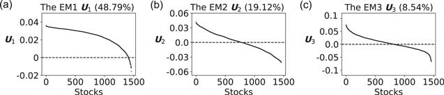New window|Download| PPT slide
Figure 21.The largest three eigen microstates U₁,U₂ and U₃ with respect to stocks.

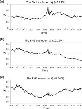
Figure 22.

New window|Download| PPT slide
Figure 22.Evolutions of the largest three eigen microstates V₁,V₂ and V₃.


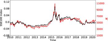
The EM1 evolution V₁ resembles the SSE100 Index perfectly with a Pearson correlation coefficient R = 0.95, as shown in figure 23. The sharp volatility during the stock market crash in 2015 can be observed both in V₁ and the SSE100 Index. As shown in figure 21(a), there are overwhelming positive components in V₁ and only 51 stocks have negative components. V₁ characterizes the main trend of the stock markets. There are 51 stocks that evolute against this trend. It can be found in the appendix table A1 that the 51 stocks come mostly from the section of coal mining.

Figure 23.

New window|Download| PPT slide
Figure 23.Comparison between the evolutions of V₁ (black line) and the SSE100 index (red line).


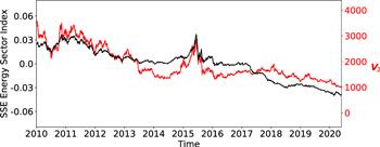
The evolution of EM2 is shown in figure 24, together with the SSE energy sector index. The Pearson correlation coefficient between them is R = 0.84. Except for the stock market crash in 2015, V₂ declines from 2010 to 2020. In U₂, About half of stocks have positive components. The top 50 stocks with positive components are listed in the appendix table A2. They are closely related to the energy sector, such as petroleum, coal and related industries. With the stocks of the SSE energy sector index marked by red dots, U₂ is presented in figure 25. The red dots have the largest positive components.

Figure 24.

New window|Download| PPT slide
Figure 24.Comparison between the evolutions of V₂ (black line) and the SSE Energy Sector Index (red line).

Figure 25.

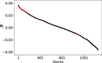New window|Download| PPT slide
Figure 25.U₂ with respect to stocks in the order of components. The stocks of the SSE Energy Index are marked by red dots.


We present the evolution of EM3 in comparison with the SSE materials sector index in figure 26. They are correlated with a Pearson correlation coefficient R = 0.75. The top 50 stocks of U₃ are listed in the appendix table A3. They come mostly from the SSE materials sector, such as steel, gold, copper, cement, etc. In figure 27 of U₃, the stocks of the SSE materials sector index are marked by red dots. It can be seen that the EM3 is dominated by the stocks of the SSE materials sector index.

Figure 26.

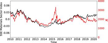New window|Download| PPT slide
Figure 26.Comparison between the evolutions of V₃ (black line) and the SSE materials sector index (red line).

Figure 27.

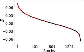New window|Download| PPT slide
Figure 27.U₃ with respect to stocks in the order of components. The stocks of the SSE Material Index are marked by red dots.


In conclusion, the eigen fluctuation patterns in stock markets have been captured by the eigen microstates above. EM1 describes the general trend of the stock market. EM2 and EM3 are related to the evolutions of the energy and material sectors in the stock market. The hierarchical features of stock market have been exhibited by the eigen microstates.

5. Conclusions

We provide a framework to study emergence behaviors in equilibrium and non-equilibrium complex systems. For a complex system with N agents, we can compose a statistical ensemble with M microstates described by N-dimensional vectors with components defined by fluctuations of agents. The ensemble is described by an N × M normalized matrix A. We can decompose the matrix as ${\boldsymbol{A}}={\sum }_{I=1}^{r}{\sigma }_{I}{{\boldsymbol{U}}}_{I}\otimes {{\boldsymbol{V}}}_{I}$, where ${\sum }_{I=1}^{r}{\sigma }_{I}^{2}=1$ and U_I is the Ith eigen microstate with evolution described by V_I. For a complex system in disorder phase, all eigenvalues σ_I → 0 in the limits N → ∞, M → ∞. If the limit of σ_I becomes finite, there is a condensation of the eigen microstate U_I in analogy to the Bose-Einstein condensation of Bose gases. This indicates a phase transition of the complex system with the order parameter given σ_I and the new phase described by U_I. Our method can be applied to both equilibrium and non-equilibrium complex systems.

For the three-dimensional Ising model in equilibrium, we have studied its eigen microstates and the corresponding eigenvalues in different temperatures. With the decrease of temperature, the largest microstate U₁ of the Ising model changes from disorder to ferromagnetic. The eigenvalue σ₁ becomes finite also. This indicates that there is a condensation of ferromagnetic microstate and a ferromagnetic phase transition. Our Monte Carlo simulation data have confirmed that the eigenvalues σ_I follow a finite-size scaling for temperatures near the critical point.

The eigen microstates of non-equilibrium complex systems including the Earth system and stock markets are studied. For the Earth system, the temperature microstates between 01-January-1950 and 31-December-2018 have been investigated. U₁ contributes about 54% of the total temperature variance. It reveals a classic solstitial mode, which reflects the impact of anti symmetric annual solar forcing with a one-to-two-month phase delay in the atmospheric response. Its spatial distribution exhibits an inter-hemisphere contrast. U₂ contributes about 11% of the total temperature variance. It reveals a remarkable land-sea temperature contrast resulted by the land-sea thermal capacity difference. We have shown that U₂ is correlated with monsoons. U₃ is featured as the climate fluctuation within the tropics. It has a dominant period of 0.5 year, which is resulted by the maximum solar forcing due to the Sun crossing the equator twice a year. We find a tipping point of V₃ in consistence with the well-known 1976-1977 climate shift. U₄ is mainly located in the tropics and high latitudes. V₄ is dominated by a semiannual signal, which is related to the so-called SAO in meteorology. U₅ is related to the ENSO, and its evolution V₅ resembles the ONI. In addition, we have studied the microstates of stock markets in Chinese mainland with the stock data from 04-January-2010 to 26-May-2020. The first eigen microstate resembles the SSE100 Index with a Pearson correlation coefficient R = 0.95. The second and third eigen microstates are correlated with the SSE Sector Indices of energy and materials, respectively.

This eigen microstate method can be applied to other non-equilibrium complex systems [44, 45]. It is expected that phase transitions of collective motion [50, 51] and tipping points in climate systems [52] and ecosystems [53] can be studied by the eigen microstate method.

Appendix

Table A1.
Table A1.The 51 stocks, which have negative components in U₁, are listed below with sectors in industry and values of component.

	Stock symbol	Industry	Value
1	600123.SH	Coal mining	−0.0156537
2	601699.SH	Coal mining	−0.0116389
3	600546.SH	Coal mining	−0.0116223
4	600256.SH	Petroleum mining	−0.0115809
5	600199.SH	Liquor	−0.0109279
6	600403.SH	Coal mining	−0.0101699
7	600348.SH	Coal mining	−0.0099700
8	600971.SH	Coal mining	−0.0097196
9	000937.SZ	Coal mining	−0.0083262
10	600691.SH	Pesticide fertilizer	−0.0081774
11	000157.SZ	Construction machinery	−0.0080799
12	000799.SZ	Liquor	−0.0079999
13	000983.SZ	Coal mining	−0.0078971
14	600508.SH	Coal mining	−0.0077700
15	601666.SH	Coal mining	−0.0077409
16	600997.SH	Coal mining	−0.0077055
17	600844.SH	Chemical raw materials	−0.0072676
18	600188.SH	Coal mining	−0.0070650
19	600031.SH	Construction machinery	−0.0067909
20	601001.SH	Coal mining	−0.0065050
21	600132.SH	Beer	−0.0058330
22	000968.SZ	Coal mining	−0.0054416
23	002069.SZ	Fishery	−0.0053891
24	000809.SZ	Regional real estate	−0.0053213
25	002106.SZ	Components	−0.0052831
26	600395.SH	Coal mining	−0.0048973
27	600381.SH	Medical care	−0.0044463
28	000869.SZ	Red and yellow wine	−0.0043872
29	601958.SH	Small metals	−0.0036315
30	600809.SH	Liquor	−0.0036107
31	600111.SH	Small metals	−0.0035444
32	002128.SZ	Coal mining	−0.0030434
33	000933.SZ	Coal mining	−0.0029023
34	600779.SH	Liquor	−0.0027581
35	600362.SH	Copper	−0.0026821
36	000960.SZ	Small metals	−0.0025779
37	600141.SH	Chemical raw materials	−0.0023876
38	002140.SZ	Construction engineering	−0.0023799
39	600740.SH	Coke processing	−0.0019607
40	600121.SH	Coal mining	−0.0019506
41	600375.SH	Automobiles	−0.0018485
42	000962.SZ	Small metals	−0.0018200
43	600547.SH	Gold	−0.0015524
44	002155.SZ	Gold	−0.0012866
45	600096.SH	Pesticide fertilizer	−0.0012306
46	000338.SZ	Auto parts	−0.0011826
47	600801.SH	Cement	−0.0005575
48	601088.SH	Coal mining	−0.0005393
49	600600.SH	Beer	−0.0005185
50	600875.SH	Electrical equipment	−0.0003222
51	600489.SH	Gold	−0.0001693

New window|CSV


Table A2.
Table A2.List of the top 50 stocks with positive components of U₂ and sectors in industry. They are closely related to the energy sector of industry.

	Stock symbol	Industry	Value
1	002069.sz	Fishery	0.0550643
2	600096.sh	Pesticide fertilizer	0.0528409
3	600121.sh	Coal mining	0.0524364
4	002269.sz	Apparel	0.0524142
5	600858.sh	Department stores	0.0520945
6	000655.sz	General steel	0.0518988
7	000809.sz	Regional real estate	0.0517208
8	600509.sh	Thermal power generation	0.0516920
9	600331.sh	Lead-zinc	0.0514581
10	000962.sz	Small metals	0.0514527
11	600644.sh	Hydropower	0.0513471
12	002073.sz	Software services	0.0513363
13	600397.sh	Coal mining	0.0512892
14	300022.sz	Agricultural machinery	0.0509761
15	600375.sh	Automobiles	0.0508973
16	600333.sh	Gas and heating	0.0504784
17	600778.sh	Department stores	0.0504760
18	000862.sz	New electric power	0.0501137
19	600166.sh	Automobiles	0.0499687
20	600078.sh	Chemical raw materials	0.0499670
21	600251.sh	Agricultural complex	0.0499422
22	600307.sh	General steel	0.0498540
23	600844.sh	Chemical raw materials	0.0497993
24	000969.sz	Steel processing	0.0496595
25	601005.sh	General steel	0.0494886
26	600875.sh	Electrical equipment	0.0493948
27	002140.sz	Construction engineering	0.0492951
28	600403.sh	Coal mining	0.0492887
29	600425.sh	Cement	0.0487832
30	002225.sz	Other building materials	0.0487225
31	600724.sh	Cement	0.0484018
32	600395.sh	Coal mining	0.0483786
33	600792.sh	Coke processing	0.0483285
34	600381.sh	Medical care	0.0482970
35	601001.sh	Coal mining	0.0482963
36	600467.sh	Fishery	0.0482299
37	600582.sh	Construction machinery	0.0477340
38	000960.sz	Small metals	0.0476099
39	000893.sz	Food	0.0475348
40	601918.sh	Coal mining	0.0474391
41	600616.sh	Red and yellow wine	0.0469954
42	600058.sh	Business agency	0.0468971
43	600537.sh	Semiconductor	0.0467404
44	002029.sz	Apparel	0.0467173
45	601958.sh	Small metals	0.0467052
46	000557.sz	Railway	0.0465262
47	000937.sz	Coal mining	0.0464698
48	601898.sh	Coal mining	0.0464407
49	600339.sh	Petroleum processing	0.0461237
50	300029.sz	Special machinery	0.0460201

New window|CSV


Table A3.
Table A3.List of the top 50 stocks with positive components of U₃ and sectors in industry. They are closely related to the raw materials sector of industry.

	Stock symbol	Industry	Value
1	000401.SZ	Cement	0.0745595
2	000425.SZ	Construction machinery	0.0733337
3	600231.SH	General steel	0.0732387
4	600581.SH	General steel	0.0711848
5	000877.SZ	Cement	0.0710412
6	600456.SH	Small metals	0.0709966
7	600729.SH	Department stores	0.0704835
8	601899.SH	Gold	0.0703957
9	601088.SH	Coal mining	0.0698539
10	600132.SH	Beer	0.0688951
11	000968.SZ	Coal mining	0.0688016
12	002083.SZ	Textile	0.0668737
13	600547.SH	Gold	0.0668275
14	600859.SH	Department stores	0.0659839
15	600295.SH	Small metals	0.0656441
16	000898.SZ	General steel	0.0650409
17	000528.SZ	Construction machinery	0.0649777
18	601111.SH	Air transport	0.0648821
19	600326.SH	Cement	0.0642478
20	600449.SH	Cement	0.0638847
21	600810.SH	Chemical fiber	0.0633524
22	000597.SZ	Chemical pharmacy	0.0631210
23	600720.SH	Cement	0.0630507
24	000546.SZ	Cement	0.0624129
25	000703.SZ	Chemical fiber	0.0619837
26	000918.SZ	National real estate	0.0611608
27	002128.SZ	Coal mining	0.0610831
28	000933.SZ	Coal mining	0.0609055
29	600362.SH	Copper	0.0603090
30	000338.SZ	Auto parts	0.0602836
31	600216.SH	Chemical pharmacy	0.0602699
32	002110.SZ	General steel	0.0601954
33	002092.SZ	Chemical raw materials	0.0601682
34	600970.SH	Construction engineering	0.0596964
35	000951.SZ	Automobiles	0.0593858
36	600239.SH	Regional real estate	0.0590865
37	601168.SH	Copper	0.0585304
38	000825.SZ	Special steel	0.0581011
39	600188.SH	Coal mining	0.0578562
40	002088.SZ	Mineral products	0.0578412
41	600308.SH	Papermaking	0.0575344
42	600888.SH	Aluminum	0.0573318
43	000617.SZ	Diversified finance	0.0571679
44	600508.SH	Coal mining	0.0571411
45	600997.SH	Coal mining	0.0571142
46	601600.SH	Aluminum	0.0567971
47	000822.SZ	Chemical raw materials	0.0565928
48	601003.SH	General steel	0.0560530
49	600068.SH	Construction engineering	0.0560270
50	600569.SH	General steel	0.0555972

New window|CSV

Acknowledgments

This work was supported by the Key Research Program of Frontier Sciences, Chinese Academy of Sciences (Grant No. QYZD-SSW-SYS019) and the HPC Cluster of ITP-CAS. We also acknowledge Naiming Yuan and Jiaqi Dong for discussions.

Reference View Option By original order
By published year
By cited within times
By Impact factor

[1]Castellano C, Fortunato S, Loreto V 2009 Rev. Mod. Phys. 81 591
DOI:10.1103/RevModPhys.81.591 [Cited within: 1]

[2]Yakovenko V M, Rosser J B 2009 Rev. Mod. Phys. 81 1703
DOI:10.1103/RevModPhys.81.1703 [Cited within: 1]

[3]Muñoz M A 2018 Rev. Mod. Phys. 90 031001
DOI:10.1103/RevModPhys.90.031001 [Cited within: 1]

[4]Gibbs J W 1902 Elementary Principles in Statistical Mechanics New York Charles Scribner’s Sons 6
[Cited within: 2]

[5]Huang W L, Li J, Chen X 2019 Ind. Eng. Chem. Res. 58 12478
DOI:10.1021/acs.iecr.9b01655 [Cited within: 1]

[6]Hu G, Liu T, Liu M, Chen W, Chen X 2019 Sci. China Phys. Mech. Astron. 62 990511
DOI:10.1007/s11433-018-9353-x [Cited within: 9]

[7]Strang G 2009 Introduction to Linear Algebra Wellesley Cambridge Press 284
[Cited within: 1]

[8]Li X, Chen X 2016 Commun. Theor. Phys. 66 355
DOI:10.1088/0253-6102/66/3/355 [Cited within: 2]

[9]Fan J, Liu M, Li L, Xi Chen 2012 Phys. Rev. E 85 061110
DOI:10.1103/PhysRevE.85.061110 [Cited within: 1]

[10]Wolff U 1989 Phys. Rev. Lett. 62 361
DOI:10.1103/PhysRevLett.62.361 [Cited within: 2]

[11]Ferrenberg A M, Landau D P 1991 Phys. Rev. B 44 5081
DOI:10.1103/PhysRevB.44.5081 [Cited within: 1]

[12]Liu A J, Fisher M E 1989 Physica A 156 35
DOI:10.1016/0378-4371(89)90109-X [Cited within: 1]

[13]Zhang X, Hu G, Zhang Y, Li X, Chen X 2018 Sci. China Phys. Mech. Astron. 61 120511
DOI:10.1007/s11433-018-9266-x [Cited within: 1]

[14]Fan J, Meng J, Ludescher J, Chen X, Ashkenazy Y, Kurths J, Havlin S, Schellnhuber H J 2021 Phys. Rep. 896 1
DOI:10.1016/j.physrep.2020.09.005 [Cited within: 1]

[15]Fan J, Meng J, Ashkenazy Y, Havlin S, Schellnhuber H J 2017 Proc. Natl Acad. Sci. 114 7543
DOI:10.1073/pnas.1701214114 [Cited within: 1]

[16]Meng J, Fan J, Ludescher J, Agarwal A, Chen X, Bunde A, Kurths J, Schellnhuber H J 2020 Proc. Natl Acad. Sci. 117 177
DOI:10.1073/pnas.1917007117 [Cited within: 1]

[17]Zhang Y, Fan J, Li X, Liu W, Chen X 2020 New J. Phys. 22 093077
DOI:10.1088/1367-2630/abb89a [Cited within: 1]

[18]Kalnay E et al. 1996 Bull. Am. Meteorol. Soc. 77 437
DOI:10.1175/1520-0477(1996)077<0437:TNYRP>2.0.CO;2 [Cited within: 1]

[19]Wang B, Ding Q 2006 Geophys. Res. Lett. 33 L06711
DOI:10.1029/2005GL025347 [Cited within: 3]

[20]Ramage C 1971 Monsoon Meteorology New York Academic 153
[Cited within: 1]

[21]Suppiah R 1992 Prog. Phys. Geogr. 16 283
DOI:10.1177/030913339201600302 [Cited within: 1]

[22]Sultan B, Janicot S, Sultan B, Janicot S 2003 J. Clim. 16 3407
DOI:10.1175/1520-0442(2003)016<3407:TWAMDP>2.0.CO;2 [Cited within: 1]

[23]Adams D K, Comrie A C 1997 Bull. Am. Meteorol. Soc. 78 2197
DOI:10.1175/1520-0477(1997)078<2197:TNAM>2.0.CO;2 [Cited within: 1]

[24]Carvalho L M V, Jones C, Silva A E, Liebmann B, Dias P L S 2011 Int. J. Climatol. 31 1248
DOI:10.1002/joc.2147 [Cited within: 1]

[25]Ha K, Heo K, Lee S, Yun K, Jhun J 2012 Meteorol. Appl. 19 200
DOI:10.1002/met.1320 [Cited within: 1]

[26]Xie S, Ahilander S G H 1994 Tellus A 46 340
DOI:10.3402/tellusa.v46i4.15484 [Cited within: 1]

[27]Philander S G H, Gu D, Lambert G, Li T, Halpern D, Lau N, Pacanowski R C 1996 J. Clim. 9 2958
DOI:10.1175/1520-0442(1996)009<2958:WTIIMN>2.0.CO;2 [Cited within: 1]

[28]Vincent D G 1994 Mon. Weather Rev. 122 1949
DOI:10.1175/1520-0493(1994)122<1949:TSPCZA>2.0.CO;2 [Cited within: 1]

[29]Mitchell T P, Wallace J M 1992 J. Clim. 5 1140
DOI:10.1175/1520-0442(1992)005<1140:TACIEC>2.0.CO;2 [Cited within: 1]

[30]Miller A J, Cayan D R, Barnett T P, Graham N E, Oberhuber J M 1994 Oceanography 7 21
DOI:10.5670/oceanog.1994.11 [Cited within: 1]

[31]Loon H V 1967 J. Atmos. Sci. 24 472
DOI:10.1175/1520-0469(1967)024<0472:THYOIM>2.0.CO;2 [Cited within: 1]

[32]Turner J, Colwell S R, Harangozo S 1997 J. Geophys. Res.: Atmos. 102 13999
DOI:10.1029/96JD03359 [Cited within: 1]

[33]Harangozo S A 1997 Tellus A 49 388
DOI:10.3402/tellusa.v49i3.14677

[34]Broeke M, Van Den R 2000 Int. J. Climatol. 20 117
DOI:10.1002/(SICI)1097-0088(200002)20:2<117::AID-JOC481>3.0.CO;2-B

[35]Broeke M R V D 2000 Int. J. Climatol. 20 455
DOI:10.1002/(SICI)1097-0088(20000330)20:4<455::AID-JOC482>3.0.CO;2-M [Cited within: 1]

[36]Schwerdtfeger W, Prohash F 1956 J. Meteorol. 13 217
DOI:10.1175/1520-0469(1956)013<0217:TSAPOI>2.0.CO;2 [Cited within: 1]

[37]Meehl G A 1991 J. Clim. 4 911
DOI:10.1175/1520-0442(1991)004<0911:AROTMO>2.0.CO;2

[38]Walland D, Simmonds I 1999 J. Clim. 12 3376
DOI:10.1175/1520-0442(1999)012<3376:BMTGAT>2.0.CO;2 [Cited within: 1]

[39]Bjerknes J 1969 Mon. Weather Rev. 97 163
DOI:10.1175/1520-0493(1969)097<0163:ATFTEP>2.3.CO;2 [Cited within: 1]

[40]Weng H, Ashok K, Behera S K, Rao S A, Yamagata T 2007 Clim. Dyn. 29 113
DOI:10.1007/s00382-007-0234-0 [Cited within: 1]

[41]Ashok K, Yamagata T 2009 Nature 461 481
DOI:10.1038/461481a [Cited within: 1]

[42]Saji N H, Goswami B N, Vinayachandran P N, Yamagata T 1999 Nature 401 360
DOI:10.1038/43854 [Cited within: 1]

[43]Cayan D R 1992 J. Phys. Oceanogr. 22 859
DOI:10.1175/1520-0485(1992)022<0859:LASHFA>2.0.CO;2 [Cited within: 1]

[44]Zhang Y, Chen D, Fan J, Havlin S, Chen X 2018 Europhys. Lett. 122 58003
DOI:10.1209/0295-5075/122/58003 [Cited within: 1]

[45]Zhang Y, Fan J, Chen X, Ashkenazy Y, Havlin S 2019 Geophys. Res. Lett. 46 12476
DOI:10.1029/2019GL084649 [Cited within: 1]

[46]Barmatz M, Hahn I, Lipa J A, Duncan R V 2007 Rev. Mod. Phys. 79 1
DOI:10.1103/RevModPhys.79.1 [Cited within: 1]

[47]Didier S 2014 Rep. Prog. Phys. 77 062001
DOI:10.1088/0034-4885/77/6/062001 [Cited within: 1]

[48]Laloux L, Cizeau P, Bouchaud J P, Potters M 1999 Phys. Rev. Lett. 83 1467
DOI:10.1103/PhysRevLett.83.1467 [Cited within: 1]

[49]Yan Y, Liu M, Zhu X, Chen X 2012 Chin. Phys. Lett. 29 028901
DOI:10.1088/0256-307X/29/2/028901 [Cited within: 1]

[50]Vicsek T, Czirók A, Ben-Jacob E, Cohen I, Shochet O 1995 Phys. Rev. Lett. 75 1226
DOI:10.1103/PhysRevLett.75.1226 [Cited within: 1]

[51]Grégoire G, Chaté H 2004 Phys. Rev. Lett. 92 025702
DOI:10.1103/PhysRevLett.92.025702 [Cited within: 1]

[52]Lenton T M, Held H, Kriegler E, Hall J W, Lucht W, Rahmstorf S, Schellnhuber H J 2008 Proc. Natl Acad. Sci. USA 105 1786
DOI:10.1073/pnas.0705414105 [Cited within: 1]

[53]Scheffer M et al. 2012 Science 338 344
DOI:10.1126/science.1225244 [Cited within: 1]