| Fund supported: |

Abstract
Keywords:
PDF (247KB)MetadataMetricsRelated articlesExportEndNote|Ris|BibtexFavorite
Cite this article
Wen-Ge Wang. A Renormalized-Hamiltonian-Flow Approach to Eigenenergies and Eigenfunctions *. [J], 2019, 71(7): 861-868 doi:10.1088/0253-6102/71/7/861
1 Introduction
Properties of energy eigenvalues and eigenfunctions are of central importance in a variety of fields, from nuclei physics, atomic physics, to condensed matter physics, and so on.[1-12] In particular, they are of relevance to thermalization,[13-21] a topic which has attracted renewed interest in recent years. An important method of studying these properties is the renormalization group method. Various versions of this method have been developed. For example, in calculating energy eigenfunctions in the low energy region, wide use has been made of Wilson's numerical renormalization group[22-23] and of the density-matrix renormalization group method.[24-25]Localization of wavefunctions is one of the most important phenomena discovered in the field of condensed matter physics[26-30] and in the field of quantum chaos.[31-32] A real-space renormalization-group method and its modified versions[33-38] have been found quite successful in the study of localization properties in one-dimensional systems with (effectively) finite range of coupling; while in the case of two and more than two-dimensional systems, they have been found successful only in some special cases such as the Fibonacci quasi-lattices (see, e.g., Refs. [39--40]). Moreover, recently, the phenomenon of many-body location has attracted wide attention (see, e.g., Refs. [41--44]).
Different schemes of constructing renormalized Hamiltonian flows are usually suitable for different types of problems. No scheme has been found universally useful. Hence, it is always of interest to find new schemes of constructing renormalized Hamiltonian flows.
In this paper we introduce a new method of constructing renormalized Hamiltonian flow, based on a generalized Brillouin-Wigner perturbation theory (GBWPT).[45-49] The GBWPT shows that an arbitrary eigenfunction of a Hamiltonian can be divided into two parts, a perturbative part and a non-perturbative part, with the perturbative part expanded in a convergent perturbation expansion in terms of the non-perturbative part. Making use of this result of the GBWPT, we show that a subspace of the Hilbert space, which is associated with a perturbative part of the eigenfunction, can be decimated. This decimation scheme produces a renormalized Hamiltonian and, following this procedure, a renormalized Hamiltonian flow can be constructed.
We show that, for a renormalized Hamiltonian flow constructed by the method mentioned above, eigenenergies of the original Hamiltonian appear as (unstable) fixed points of a property of the flow. Furthermore, those eigenfunctions of the renormalized Hamiltonians in the flow, which share the same eigenenergy, have related components. These two properties of the renormalized Hamiltonian flow may be made use of in approximate calculation of eigenenergies and in the study of properties of the eigenfunctions of the original Hamiltonian, e.g., their localization properties. These predictions are checked numerically in the Wigner-band random-matrix model.
2 General Theory
2.1 Generalized Brillouin-Wigner Perturbation Theory
In this section, we discuss the basic contents of GBWPT. It is a direct generalization of the ordinary Brillouin-Wigner perturbation theory, which can be found in textbooks, e.g., in Ref. [50]. Consider a perturbed Hamiltonian $H = H_0 +V$, where $H_0$ is an unperturbed Hamiltonian and $V$ is a generic perturbation. In the normalized eigenbasis of $H_0$, denoted by $|k\rangle $,Here, ${E}^0_k = \langle k| H_0|k \rangle $, ${V}_{kk'} = \langle k |H| k' \rangle $ for $k \ne k'$, and, without the loss of generality, we assume that $V_{kk'}=0$ for $k=k'$. (In the case that $V$ has non-zero diagonal elements in the basis of $|k\rangle $, one may adjust $H_0$ to absorb the diagonal part of $V$.) We use $|\alpha \rangle $ and $E_{\alpha }$ to denote the eigenstates and eigenenergies of $H$, $ H |\alpha \rangle =E_{ \alpha }| \alpha \rangle $. The components of $|\alpha \rangle $ in $|k\rangle $ are written as $C_{\alpha k} \equiv \langle k|\alpha \rangle $.
For an energy eigenstate $|\alpha \rangle $, let us divide the set $\{|k\rangle \}$ into two subsets, denoted by $S_{\alpha }$ and ${\bar S}_{\alpha }$, respectively. This gives two projection operators $P$ and $Q $,
Here we use $|i\rangle $ to indicate basis states $|k\rangle $ in $ S_{\alpha }$ and $|j\rangle $ for $|k\rangle \in {\bar S}_{\alpha }$. Correspondingly, the state $|\alpha \rangle $ is divided into two parts,
where $ |{\alpha }_s\rangle \equiv P|\alpha \rangle$ and $ |\alpha _{\bar s}\rangle \equiv Q |\alpha \rangle $. One can write the stationary Schr?dinger equation in the following form,
Multiplying both sides of Eq. (4) by $Q$ and noticing that $QH_0 = H_0Q$, one has
where
when the following condition is satisfied
When the set $S_\alpha$ includes only one basis vector $|i\rangle $, the expansion in Eq. (7) gives the ordinary Brillouin-Wigner perturbation expansion. Since the exact eigenenergy $E_\alpha$ appears in the expansion, the expansion can not be immediately employed in numerical computation. However, noticing that $|\alpha_s\rangle $ has one component only in the basis $|i\rangle $ and that the components $C_{\alpha k}$ should satisfy certain normalization condition, this problem can be overcome. For example, taking the normalization condition $\langle i |\alpha\rangle =1$ for normalized $|i\rangle $ and multiplying Eq. (4) from left by $\langle i|$, one can write the exact energy as $E_\alpha = E_i^0 + \langle i| V|\alpha \rangle $. Then, one can write $E_\alpha$ and $|\alpha\rangle $ in the form of two related iterative expansions.[50]
In the case that $S_\alpha$ includes more than one vectors $|i\rangle $, Eq. (7) gives a generalization of the (ordinary) Brillouin-Wigner perturbation theory (GBWPT). In this case, since there are at least two components $C_{\alpha i}$ in $|\alpha_s\rangle $, merely making use of the normalization condition, one can not write $E_\alpha$ and $|\alpha\rangle $ in two related iterative expansions. Therefore, in the GBWPT, $E_\alpha$ and $|\alpha\rangle $ can not be calculated in a way similar to that discussed above in the ordinary Brillouin-Winger perturbation theory.
Several applications of the GBWPT have been found. The condition (8) determines the separation of $|\alpha\rangle $ into two parts, $|\alpha_s\rangle $ and $|\alpha_{\bar s }\rangle $. In systems with band structure of the Hamiltonian, usually $|\alpha_s \rangle $ corresponds to the main body of $|\alpha\rangle $, while $|\alpha_{\bar s }\rangle $ corresponds to the tail part of $|\alpha\rangle $ with small components.[45,48] It has been shown that the expansion in Eq. (7) is useful in deriving analytical expressions for the decaying behavior of the tails of $|\alpha\rangle $.[45,48] This separation of $|\alpha\rangle $ has also been found useful in approximate calculation of eigenstates in certain energy region.[47] Further numerical investigation reveals that this separation of energy eigenstates is useful in the study of phenomenon like dynamical localization[46,48] and in the study of the distribution of components of wave functions in quantum chaotic systems.[49]
In order to understand better the condition (9), we insert the expression of the projection operator $Q$ given in Eq. (2) into Eq. (6) and get
An advantage of using Eq. (9) is that one does not need to know the exact state $|\alpha \rangle $ in advance. Equation (9) is also useful when we treat a Hamiltonian $H$ with a degenerate spectrum. As well known, degenerate spectrum of $H$ may bring problem to the ordinary perturbation theory. However, in the GBWPT, Eq. (7) can still hold when $H$ has a degenerate spectrum. In fact, since Eq. (9) does not contain any eigenstate, for eigenstates with the same eigenenergy $E_\alpha$, this equation gives the same separation of the basis states $|k\rangle $, i.e., the set $S_\alpha$. For such a separation, Eq. (7) holds for all the eigenstates with the eigenenergy $E_\alpha$. In this case, $S_\alpha$ includes more than one basis vectors. Different eigenstates $|\alpha\rangle $ with the same eigenvalue $E_\alpha$ have different components $C_{\alpha i}$ in $|\alpha_s\rangle $, hence, have different $|\alpha_{\bar s }\rangle $ determined by Eq. (7).
For the above reasons, in what follows, we use Eq. (9) to determine the separation of $|\alpha\rangle $ into the two parts $|\alpha_s\rangle $ and $|\alpha_{\bar s }\rangle $.
2.2 Renormalized Hamiltonian
A renormalized Hamiltonian can be constructed for an eigenstate $|\alpha \rangle $ of $H$, by decimation of the states $|j\rangle $ in ${\bar S}_{\alpha }$. For this purpose, making use of Eq. (7), we write $C_{\alpha j} =\langle j|\alpha \rangle =\langle j|\alpha_{\bar s } \rangle $ aswhere
In the stationary Schr?dinger equation
replacing $C_{\alpha j}$ by the right hand side of Eq. (11), one has
where
This suggests that a renormalized Hamiltonian $\tilde{H} $ can be introduced,
which is an operator in the subspace spanned by states $|i\rangle \in S_{\alpha }$. The most important relation between $H$ and $\tilde{H}$ is that the state $( \sum_i C_{\alpha i}|i\rangle ) $ is an eigenstate of $\tilde{H}$ with the eigenenergy $E_{\alpha }$, as shown in Eq. (14). Note that the elements $\tilde{H}_{ii'}$ are functions of $E_{\alpha }$.
When $H$ has a degenerate spectrum, as discussed in the previous section, degenerate eigenstates with the same eigenenergy $E_\alpha$ share the same separation $S_\alpha$, hence, they have the same quantities $ A_{\alpha }(j \to i')$. As a result, degenerate eigenstates $|\alpha\rangle $ are eigenstates of the same renormalized Hamiltonian $\tilde{H}$. Therefore, the above scheme also works in the case of degenerate spectrum.
The structure of non-zero off-diagonal elements of $H$ in the basis $|k\rangle $ is usually different from that of ${\tilde{H}}$ in $|i\rangle $. Indeed, Eqs. (12) and (15) show that ${\tilde{H}}_{ii'}$ is typically non-zero when either $H_{ii'} \ne 0$ or there is a path of coupling from $|i\rangle $ to $|i'\rangle $ through states $|j\rangle $ in the set ${\bar S}_{\alpha }$. Therefore, the number of basis states $|i'\rangle $ which are coupled to $|i\rangle $ by ${\tilde{H}}$ is equal to or larger than that by $H$.
We remark that the condition (8), which guarantees the expansion in Eq. (7), can not completely fix the set $S_{\alpha}$. Hence, one usually has much free space in choosing $S_{\alpha }$ in constructing a renormalized Hamiltonian.
2.3 Renormalized Hamiltonian Flow
Repeating the procedure discussed in the previous section, with $\tilde{H}$ playing the role of $H$, one can obtain a new renormalized Hamiltonian from $\tilde{H}$. Following this, a renormalized Hamiltonian flow can be constructed, which is specific for the eigenstate $|\alpha \rangle $ with eigenenergy $E_{\alpha}$ of the original Hamiltonian $H$. However, this method of constructing Hamiltonian flow has a drawback, namely, $|\alpha\rangle $ and $E_{\alpha}$ are usually unknown. (The purpose of constructing a renormalized Hamiltonian flow is usually just to study properties of $|\alpha\rangle $ and $E_{\alpha}$.) To avoid this drawback, in what follows we propose a more general method of constructing renormalized Hamiltonian flow, which is not specific for any eigensolution of $H$.Let us denote by $H^{(0)}$ the original Hamiltonian $H$, by $E_{\alpha^{(0)}}$ and $|\alpha^{(0)}\rangle $ its eigenenergies and eigenstates, respectively. For a set of basis states in the Hilbert space of $H^{(0)}$, denoted by $\{ |k^{(0)}\rangle \}$, $H^{(0)}$ is divided into two parts as in Eq. (1), $H^{(0)}= H_0^{(0)}+V^{(0)}$. The set of basis states is also divided into two parts $S^{(0)}$ and $\bar S^{(0)}$, with $|i^{(0)}\rangle \in S^{(0)}$ and $|j^{(0)}\rangle \in \bar S^{(0)}$; correspondingly, two projection operators $P^{(0)}$ and $Q^{(0)}$ can be introduced in the same way as in Eq. (1). The components of $|\alpha^{(0)}\rangle $ are denoted by $C_{\alpha^{(0)} k^{(0)}} = \langle k^{(0)}| \alpha^{(0)}\rangle $.
In considering the condition for a division of $\{ |k^{(0)}\rangle \}$, let us write Eq. (9) in the following form,
where
Here $E$ is a parameter with energy dimension, which is used in the construction of the renormalized Hamiltonian flow. Note that Eq. (17) gives Eq. (9) for $E=E_{\alpha}$.
Then, we can decimate the basis states in $\bar S^{(0)}$ and, similar to $\tilde{H}$ in Eq. (16), introduce the first renormalized Hamiltonian $H^{(1)}_E$ in the flow,
where
Here
For $E=E_{\alpha^{(0)}}$, similar to Eq. (14), we have
hence, $E_{\alpha^{(0)}}$ is an eigenenergy of $H^{(1)}_E$ with $E=E_{\alpha^{(0)}}$. If $E$ is not equal to any of $E_{\alpha^{(0)}}$, it is usually not an eigenenergy of $H^{(1)}_E$. Note that $H^{(1)}_E$ is an operator in the Hilbert space spanned by $|k^{(0)}\rangle \in S^{(0)}$.
In the above procedure, with the superscript $(0)$ replaced by Eq. (1), the second renormalized Hamiltonian $H^{(2)}_E$ in the flow can be constructed for the same parameter $E$. Then, with the superscript (1) replaced by Eq. (2), and so on, a renormalized Hamiltonian flow $H^{(n)}_E$ can be constructed, with $n=1,2, \ldots $
If $E=E_{\alpha^{(0)} }$ for a Hamiltonian flow thus obtained, an equation similar to Eq. (22) holds with 0 replaced by $n-1$ and 1 by $n$. This implies the following important relation between $H^{(n)}_E$ and $H^{(0)}$, that is, an eigenstate $|\alpha ^{(n)} \rangle $ of $H^{(n)}_E$ has the following relation to $|\alpha^{(0)} \rangle $,
where $|k^{(0)}\rangle $ is the same basis state as $|k^{(n)} \rangle $ but in the original labelling. This equation shows that some information in properties of $|\alpha^{(0)} \rangle $ may be obtained from properties of the corresponding eigenstate $| \alpha ^{(n)} \rangle$ of $H^{(n)}_E$.
In the general case with $E$ not necessarily equal to any of $E_{\alpha^{(0)} }$, let us denote by $E^{(n)}$ the closest eigenenergy of $H^{(n)}_E$ to $E$. (For $n=0$, take $H^{(0)}$). With increasing $n$, $E^{(n)}$ form a sequence with the flow, ($E^{(0)},E^{(1)},E^{(2)},\ldots$). If $E=E_{\alpha^{(0)} }$, Eq. (23) shows that $E^{(n)}= E_{\alpha^{(0)}}$ for all values of $n$; on the other hand, if $E \ne E_{\alpha^{(0)} }$, $E^{(n)}$ are usually not equal to $E_{\alpha^{(0)}}$. Hence, $E_{\alpha^{(0)} }$ are fixed points of the sequence $E^{(n)}$, under the choice of $E=E_{\alpha^{(0)} }$. One may also consider the sequence of the deviation $|E_{\alpha^{(n)}}-E|$, for which zero is the fixed point corresponding to the choice $E=E_{\alpha^{(0)} }$.
2.4 An Efficient Method of Constructing Renor-malized Hamiltonian Flow
The condition (17) with 0 replaced by $n$ must be satisfied, in order to construct $H^{(n+1)}_E$ from $H^{(n)}_E$ by decimating basis states $|j^{(n)}\rangle $ in ${\bar S}^{(n)}$. For a given choice of ${\bar S}^{(n)}$, it is usually not easy to prove whether the condition is satisfied or not. In fact, for an arbitrarily chosen set ${\bar S}^{(n)}$ and an arbitrary value of $E$, the condition is usually not satisfied. Therefore, it would be useful, if a general method can be found for decimation of an arbitrarily chosen set ${\bar S}^{(n)}$. In what follows, we introduce such a method. For brevity, in the following part of this section, we omit the superscript $"(n)"$, i.e., all quantities should have the superscript $"(n)"$, except for the parameter $E$.The technique is to first carry out a rotation in the subspace spanned by states $|j\rangle \in {\bar S}$, such that $H$ is diagonalized in the subspace. We assume that the number of states in ${\bar S}$ is not large and it is not difficult to diagonalize numerically the sub-matrix of the Hamiltonian $H$ in this subspace. Let us denote by $|j_a\rangle $ the obtained eigenstates of the sub-matrix of $H$ in the subspace and by $E_{j_a}$ the corresponding eigenenergies.
Now take the set of $|j_a\rangle $ as a new subset $\bar S$. Correspondingly, the Hamiltonian $H$ is divided into two parts, $H_0$ and $V$, in the same way as discussed in previous sections. In particular, by definition, $|j_a\rangle$ is an eigenstate of $H_0$,
Then, making use of the expression of $Q$ in Eq. (2), we can write $T_E$ in Eq. (18) as (with the superscript (0) replaced by $(n)$ and then omitted)
when $E$ is not equal to any of $ E_{j_a}$. Equation (25) implies that $(T_E)^2=0$, since there is no coupling among $|j_a\rangle $, namely, $\langle j_a |V |{j_a}' \rangle =0$. As a result, Eq. (17) holds with 0 replaced by $n$. When it happens that $E$ is equal to one of $E_{j_a}$, one may change a little the two original subsets $S$ of $|i\rangle $ and $\bar S$ of $|j\rangle $ by exchanging a few states in them; this may change the values of $E_{j_a}$ and make $E \ne E_{j_a}$.
Finally, by the method discussed in the previous section, the set of $|j_a\rangle $ (equivalently, that of $|j \rangle $) can be decimated and a renormalized Hamiltonian can be obtained. In particular, $A_E(j_a \to i)$ has a quite simple expression,
since $(T_E)^2=0$ for the choice of the set of $|j_a\rangle$. It is not difficult to see that the above schemes can work for a degenerate spectrum, as well.
3 Some Applications
In this section, we show that the method presented in this paper supplies a useful approach to properties of energy eigenvalues and eigenfunctions.3.1 Eigenenergies as Unstable Fixed Points
As discussed in Subsec. 2.3, the eigenenergies $E_{\alpha^{(0)}}$ of the original Hamiltonian $H^{(0)}$ are fixed points of the sequence $E^{(n)}$, where $E^{(n)}$ is the eigenenergy of $H^{(n)}_E$ which is the closest to $E$. As a result of this property, the difference $|E-E^{(n)}|$ as a function of $E$ (with $n$ fixed) has local minima at the positions $E=E_{\alpha^{(0)}}$. Hence, the eigenenergies $E_{\alpha^{(0)}}$ can be calculated by finding out the local minima. In fact, numerical evaluation of eigenenergies of large-scale Hamiltonian matrices is a very important topic in many fields in physics. Various methods have been developed in dealing with this problem (see, e.g., Refs. [47, 51--57]). The renormalization group method discussed above supplies an alternative approach to this important problem.To test the above predictions, we consider a banded random matrix model. Banded random matrix models have applications in several fields and are still under investigation (see, e.g., Refs. [58--62]). Here we consider the so-called Wigner Band Random Matrix (WBRM) model, which was first introduced by Wigner more than 50 years ago for the description of complex quantum systems as nuclei.[63] It is still of interest (see, e.g., Refs. [46, 48, 64--70]), since it is believed to provide an adequate description also for some other complex systems, e.g., the Ce atom[71] and as well as dynamical conservative systems possessing chaotic classical limits.
We consider the following form of the Hamiltonian matrix in the WBRM model,
where $ E^0_k =k$ $ (k=1, \ldots , N) $, off-diagonal matrix elements $v_{kk'} = v_{k'k}$ are random numbers with Gaussian distribution for $1 \le |k-k'| \le b$ ($\langle v_{kk'} \rangle = 0$ and $\langle v^2_{kk'} \rangle =1$) and are zero otherwise, and $\lambda $ is a running parameter for adjusting the perturbation strength. Here $b$ is the band width of the Hamiltonian matrix and $N$ is its dimension.
The theory discussed above predicts that the points $E=E_{\alpha^{(0)}}$ are fixed points for the property $E^{(n)}$ of the renormalized Hamiltonian flow. To check this numerically, we consider original Hamiltonians $H^{(0)}$ as given in Eq. (27), whose dimensions are not very large such that they can be diagonalized directly by using ordinary diagonalization methods. For each $H^{(0)}$ thus obtained, we diagonalize it to obtain its eigenenergies $E_{\alpha^{(0)}}$. Then, we take $E=E_{\alpha^{(0)}}$ and construct a (finite) renormalized Hamiltonian flow $H^{(n)}_E$ by making use of the method discussed in Subsec. 2.4, with a number of arbitrarily chosen basis states $k^{(n)}$ decimated at each step. Numerically, all the renormalized Hamiltonians $H^{(n)}_E$ have been found sharing the same eigenenergy $E_{\alpha^{(0)} }$ and having related eigenfunctions, as predicted in Eq. (23).
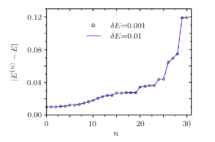
There are two types of fixed points: stable and unstable. We perform further numerical investigation to see whether the fixed points $E_{\alpha^{(0)} }$ are stable or unstable. For this, we take a value of $E$, which deviates a little from an exact eigenvalue $E_{\alpha^{(0)} }$, say by $\delta E =|E-E_{\alpha^{(0)}}|$. Variation of $|E^{(n)}-E|$ with $n$ can show whether the fixed point $E=E_{\alpha^{(0)}}$ is stable or unstable. Our numerical simulations show that they are unstable. An example is given in Fig. 1, which shows that the value of $|E^{(n)}-E|$ increases with $n$, indicating that $E_{\alpha^{(0)}}$ is an unstable fixed point. In our numerical computation for this figure, at each step of the renormalization flow, we decimated 30 basis states $|k^{(n)}\rangle $ with successive labelling $k^{(n)}$ and with the first $k^{(n)}$ chosen arbitrarily.
Fig. 1
 New window|Download| PPT slide
Fig. 1Variation of $|E^{(n)}-E|$ with $n$, for the parameters $N=1000, b=100$, and $\lambda =10$, where $E^{(n)}$ is the eigenenergy of $H^{(n)}_E$ which is the closest to $E$. The value of $E$ has a little deviation from an arbitrarily chosen exact eigenenergy $E_{\alpha^{(0)}}$ of the original Hamiltonian $H^{(0)}$. For the solid curve, $\delta E =|E-E_{\alpha^{(0)}}|=0.01$. At each step of the flow, an arbitrarily chosen set of 30 basis states with successive labelling are decimated. The value of $|E^{(n)}-E|$ increases with $n$, implying that $E_{\alpha ^{(0)}}$ is an unstable fixed point. The circles represent $|E^{(n)}-E|/10$ for $\delta E =0.001$. The agreement of the solid curve and the circles show that for these small values of $\delta E$, $|E^{(n)}-E|$ is in the linear region of $\delta E$.
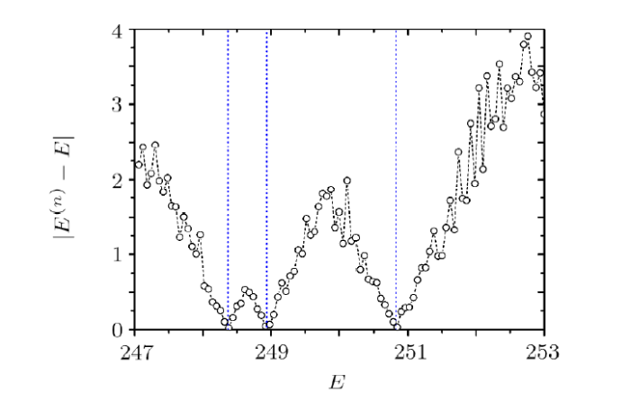
Now we study variation of $|E^{(n)}-E|$ as a function of $E$, with $n$ fixed. The theory predicts that this quantity has local minima of zero at the values of $E=E_{\alpha^{(0)}}$. Our numerical simulations indeed reveal this phenomenon. As shown in Fig. 2, the positions of the local minima with the value of zero indeed correspond to positions of the exact eigenenergies $E_{\alpha^{(0)}}$, which are indicated by the vertical dotted lines. This shows that the eigenenergies of the original Hamiltonian can be evaluated by numerical calculation of the local minima of $|E^{(n)}-E|$.
Fig. 2
 New window|Download| PPT slide
Fig. 2Variation of $|E^{(n)}-E|$ (circles connected by dashed lines) with $E$ for $n=5$, the parameters $N=300$, $b=100$, $\lambda =10$, and $E=247+0.06m$ with $m=1,2,\ldots , 100$. At each step of the renormalized Hamiltonian flow, 30 basis states are decimated. Within the energy region shown in this figure, the original Hamiltonian has three eigenenergies with positions indicated by the three vertical dotted lines. Approximate values of the eigenenergies can be get from extrapolation of the circles close to the local minima of $|E^{(n)}-E|$.
3.2 Localization of Eigenfunctions
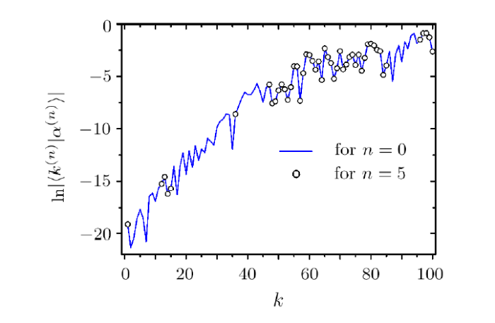
Based on Eq. (23), the theory here can also be used in the study of properties of energy eigenfunctions of $H^{(0)}$, namely, the components of $|\alpha^{(0)} \rangle $ in $| k^{(0)}\rangle$. For this, one should first know the eigenenergy $E_{\alpha^{(0)}}$, which may be obtained by the method discussed in the previous section or by some other method. Next, one can use $E=E_{\alpha^{(0)}}$ to construct a finite renormalized Hamiltonian flow, until $H_E^{(n)}$ whose dimension is small enough for direct numerical diagonalization. Then, one can perform direct numerical diagonalization for this Hamiltonian and find $\langle k^{(n)} | \alpha ^{(n)} \rangle $, which give the corresponding components of $|\alpha^{(0)} \rangle $ in $|k^{(0)}\rangle $ by the relation (23). In this way, some information about the wavefunction $\langle k^{(0)}|\alpha^{(0)} \rangle $, e.g., its localization properties, may be obtained. In fact, if data for the construction of $H^{(m)}_E$ of $m=1,\ldots , n$ have been stored, it is even possible to obtain all the components $\langle k^{(0)}|\alpha ^{(0)} \rangle $.We also employ the WBRM model discussed in the previous section to check the applicability of the method discussed above. Consider, e.g., the parameters $N=100$, $b=4$, and $\lambda =10$. Hamiltonians with these parameters have localized eigenfunctions, e.g., the one shown in Fig. 3 by the solid curve. To check the validity of Eq. (23), we first diagonalize $H^{(0)}$ directly and obtain its eigenenergies $E_{\alpha^{(0)}}$ numerically. Then, we construct a (finite) renormalized Hamiltonian flow $H^{(n)}_E$ with $E=E_{\alpha^{(0)}}$, by making use of the method discussed in Subsec. 2.4 with 10 basis states decimated at each step. Our numerical results indeed confirm the prediction of Eq. (23). An example is given in Fig. 3 for $n=5$, which shows that the values of $|\langle k^{(5)}|\alpha^{(5)} \rangle |$ agree well with the corresponding ones of $|\langle k^{(0)}|\alpha^{(0)} \rangle |$, even when $|\langle k^{(0)}|\alpha^{(0)} \rangle |$ is as small as $e^{-20}$.
Fig. 3
 New window|Download| PPT slide
Fig. 3Values of the components $|\langle k^{(n)}|\alpha^{(n)}\rangle |$ for $n=0$ and 5 in a renormalized Hamiltonian flow of $H^{(n)}_E$. The original Hamiltonian is a realization of the Hamiltonian matrix in the WBRM model with parameters $N=100$, $b=4$, and $\lambda =10$. In the construction of the renormalized Hamiltonians, $E=E_{\alpha^{(0)}}$ and 10 basis states are decimated at each step of the flow. $|\alpha^{(0)}\rangle $ and $|\alpha^{(5)}\rangle $ are eigenstates of $H^{(0)}$ and $H^{(5)}_E$, respectively, with the same eigenenergy $E_{\alpha^{(0)}}$. The two eigenfunctions agree well, as predicted in Eq. (23).
3.3 A Discussion of Computation Time
In this section, we give a brief discussion for the dependence of the computation time required by the method here on the dimension $N$ of the original Hamiltonian. This is to be compared with the corresponding dependence in ordinary direct diagonalization methods, in which the computation time usually scales as $N^3$.When using the method here to calculate eigenenergies, as discussed in Subsec. 3.1, one first needs to choose the energy region of interest and divide the region into consecutive segments, say, to $(N_s-1)$ segments. Then, one can take the $N_s$ ends of the segments as the parameter $E$ and construct renormalized Hamiltonian flows $H_E^{(n)}$. Suppose at each step totally $m$ basis states are decimated, with $m\ll N$. This requires diagonalization of an $m\times m$ matrix, which takes a time scaling as $m^3$. After decimation of the $m$ basis states, one obtains a new renormalized Hamiltonian and needs to calculate its new elements. (Some elements of the renormalized Hamiltonian may remain unchanged in the decimation process.) If there are $M_1$ new elements to be calculated and the time of calculating each new element scales as $M_2$, then, calculation of the new elements needs a time scaling as $M_1M_2$. The values of $M_1$ and $M_2$ depend on the structure of the original Hamiltonian. For example, for a 1-dimensional chain with nearest-neighbor coupling, it is possible for both $M_1$ and $M_2$ to be quite small; on the other hand, for a full original Hamiltonian, $(N^2-m^2)$ matrix elements are changed in the first step of the flow.
Suppose one performs $n$ steps of the renormalization procedure and at last obtains a final renormalized Hamiltonian of dimension $(N-nm)$. Diagonalization of the final Hamiltonian needs a time scaling as $(N-nm)^3$. Summarizing the above results, the total computation time scales as $Z = N_sn(m^3+M_1M_2)+N_s(N-nm)^3$, where for simplicity in discussion, we assume that $M_1M_2$ can be taken as a constant.
The method here is useful when a narrow energy region is of interest, because in this case $N_s$ is not large. Usually, one may choose the value of $n$ such that $nm$ is close to $N$. This gives $ Z \sim NN_s(m^2+M_1M_2/m)$. Comparing it with $N^3$ for direct diagonalization method, we see that the method here is more efficient if $N_s(m^2+M_1M_2/m) \ll N^2$. In fact, the method here has another advantage, that is, it needs a relatively small memory for diagonalization. Specifically, it needs to diagonalize matrices with dimensions $m$ and $(N-nm)$, respectively, which can be small even for large $N$. In contrast, a direct diagonalization method usually requires a memory scaling as $N^2$, which is much larger than $m^2$ and $(N-nm)^2$.
4 Conclusions and Discussions
In summary, based on the GBWPT, we propose a general method of constructing renormalized Hamiltonian flow with the energy $E$ of interest as a parameter. Eigenenergies of the original Hamiltonian appear as (unstable) fixed points of some property of the renormalized Hamiltonian flow. When $E$ is chosen as an eigenenergy of the original Hamiltonian, all the renormalized Hamiltonians in the same flow share the same eigenenergy as $E$, with the corresponding eigenfunctions possessing related components. we introduce a useful technique, by which an arbitrary set of basis states in the Hilbert space can be decimated in the construction of a renormalized Hamiltonian. We also discuss potential applications of the method in numerical evaluation of eigenenergies as well as in the study of localization of eigenfunctions, and illustrate them numerically in the WBRM model. In particular, by considering the scaling behavior of computation time, we find some situations in which the method here may be more efficient than the ordinary numerical diagonalization methods.As is known, localization in the WBRM model can be related to localization in another band-random-matrix model, by making use of a renormalization technique based on the GBWPT.[48] The method discussed in this paper can be used to improve the method in Ref. [48], specifically, by partial diagonalization of the Hamiltonian in the subspace spanned by states in ${\bar S}_{\alpha }$, without rotation in the subspace spanned by states in ${S}_{\alpha }$.
Finally, we give some remarks on the relation of the method discussed in this paper to some other methods of constructing renormalized Hamiltonians. The real-space renormalization-group method used in Refs. [33-34] for the one-dimensional tight-binding model with nearest-neighbor-hopping, is in fact a special case of the method here, with the set ${\bar S}_{\alpha }$ including only one basis state $|j\rangle $ at each step of decimation. Its modified versions for 1D or quasi-1D systems, e.g., those in Refs. [36--38], have some technical difference from the method here. A merit of the theory here is that it supplies a general approach to the construction of renormalized Hamiltonian flow, not restricted to some special types of models.
Reference By original order
By published year
By cited within times
By Impact factor
[Cited within: 1]
[Cited within: 1]
[Cited within: 1]
[Cited within: 1]
[Cited within: 1]
[Cited within: 1]
[Cited within: 1]
[Cited within: 1]
[Cited within: 1]
[Cited within: 1]
[Cited within: 1]
[Cited within: 1]
[Cited within: 2]
[Cited within: 1]
[Cited within: 1]
[Cited within: 2]
[Cited within: 1]
[Cited within: 1]
[Cited within: 1]
[Cited within: 1]
[Cited within: 3]
[Cited within: 2]
[Cited within: 2]
[Cited within: 6]
[Cited within: 2]
[Cited within: 2]
[Cited within: 1]
[Cited within: 1]
[Cited within: 1]
[Cited within: 1]
[Cited within: 1]
[Cited within: 1]
[Cited within: 1]
[Cited within: 1]
