Fund Project:Project supported by the Science Fund for Creative Research Groups of the National Natural Science Foundation of China (Grant No. 11621101) and the National Natural Science Foundation of China (Grant No. 11871429)
Received Date:03 February 2021
Accepted Date:09 March 2021
Available Online:07 June 2021
Published Online:05 July 2021
Abstract:The incompressible Navier-Stokes equations (INSE) are the basic governing equations of fluid dynamics, and their numerical solutions are of great significance. In this review paper, we first recollect some classical projection methods and their relatives in the past 50 years and then fully explain the recent fourth-order projection method called GePUP [Zhang Q 2016 J. Sci. Comput.67 1134]. Based on a generic projection operator and the UPPE formulation of the INSE [Liu J G, Liu J, Pego R L 2007 Comm. Pure Appl. Math. 60 1443], we derive the GePUP equations, which retain the advantage of UPPE that the velocity divergence is governed by a heat equation and is thus well under control. In comparison with UPPE, the GePUP formulation is advantageous in three aspects: (1) its derivation depends on none of the properties of the Leray-Helmholtz projection; (2) the evolutionary velocity can be divergent, thus it is directly applicable to numerical calculations with nonzero velocity divergence; (3) the Leray-Helmholtz projection does appear on the right-hand sides of the governing equations, thus making it transparent to analyze the accuracy and stability issues raised by numerically approximating the Leray-Helmholtz projection. As the most appealing feature of GePUP, temporal integration and spatial discretization are completely decoupled and can be treated as black boxes, so that the user can choose his favorite methods for the two parts to form his own GePUP method. In particular, high-order accuracy in time can be easily obtained since no internal details of the ODE solver are needed. The flexibility in time makes the GePUP method applicable to both low-Reynolds-number flow and high-Reynolds-number flow. The flexibility in space makes the GePUP method applicable to both rectangular boxes and irregular domains. The numerical results and elementary analysis show that the fourth-order GePUP method may be much more accurate and efficient than classical second-order projection methods by many orders of magnitude. Keywords:incompressible Navier-Stokes equations/ projection methods/ fourth-order accuracy both in time and in space/ no-slip boundary conditions/ generic projection/ pressure Poisson equation
其中$ {x}_O\in {\mathbb{R}}^{ { {{D}}}} $是固定的坐标原点, h是均匀网格间距, ${\mathds{1}}\in {\mathbb{Z}}^{ { {{D}}}}$是分量全为1的多元索引, $ {{e}}^d\in {\mathbb{Z}}^{ { {{D}}}} $表示第d个分量为1, 其余分量全为0的多元索引. 如图1所示, $ \phi $在控制体$ {\mathcal C}_{ {{i}}} $上的平均值定义为 图 1 面平均值和控制体平均值. 面平均值用带$ \left\langle {\cdot} \right\rangle $且下标为分数的符号表示, 而控制体平均值对应下标为整数. 因此 $ \left\langle {\phi} \right\rangle_{ {{i}}+\frac{1}{2} {{e}}^0} $, $ \left\langle {\phi} \right\rangle_{ {{i}}- {{e}}^0+\frac{1}{2} {{e}}^1} $和$ \left\langle {u_0} \right\rangle_{ {{i}}+\frac{3}{2} {{e}}^0 + {{e}}^1} $表示面平均值, 而$ \left\langle {\phi} \right\rangle_{ {{i}}} $是控制体平均值[5] Figure1. Notation of face-averaged and cell-averaged values. A symbol with angled brackets denotes either a cell-averaged value if the subscript is an integer multi-index, or a face-averaged value if the subscript is a fractional multi-index. Hence $ \left\langle {\phi} \right\rangle_{ {{i}}+\frac{1}{2} {{e}}^0} $, $ \left\langle {\phi} \right\rangle_{ {{i}}- {{e}}^0+\frac{1}{2} {{e}}^1} $, and $ \left\langle {u_0} \right\rangle_{ {{i}}+\frac{3}{2} {{e}}^0 + {{e}}^1} $ are face-averaged values while $ \left\langle {\phi} \right\rangle_{ {{i}}} $ is a cell-averaged value. Horizontal and vertical hatches represent the averaging processes over a vertical cell face and a horizontal cell face, respectively. Light gray area represents averaging over a cell[5].
图 4 从给定起始点开始选择一组格点以拟合多维n次完全多项式. 用拟合的完全多项式可以离散空间算子, 并且能很方便地满足边界条件[26] Figure4. For a given starting point, we choose a set of nodes to fit a high-order, multi-variate, complete polynomial, which facilitates the discretization of spatial operators and the enforcement of boundary conditions[26].
表1用GePUP-ERK算法在不规则计算域(87)上求解以(88)式和(89)式为解析解的INSE得到的误差和收敛阶. Re = 1000, $ t_0 = 0 $, $ t_{\rm e} = 0.1 $, $ {{\textsf{Cr}}} = 0.2 $[5] Table1.Errors and convergence rates of GePUP-ERK for solving the INSE on the irregular domain (87) with Eq. (88) and Eq. (89) as the analytic solutions. Re = 1000, $ t_0 = 0 $, $ t_{\rm e} = 0.1 $, $ {{\textsf{Cr}}} = 0.2 $[5].
25.2.三维顶盖驱动方腔流 -->
5.2.三维顶盖驱动方腔流
三维顶盖驱动方腔内的不可压缩流动几乎表现出流体力学中所有常见的现象: 漩涡、二次流、混沌粒子运动、不稳定性、过渡、湍流和如展向涡的复杂三维流动结构[33], 因此其数值模拟具有重要的科学意义. 另外由于几何设定非常简单, 顶盖驱动方腔流是检验INSE数值求解方法最常使用的基准测试之一. 在规则计算区域$ [0, 1]\times[0, 1]\times[0, 2] $上, 用GePUP-IMEX算法(85)式对三维顶盖驱动方腔流进行数值模拟. 选择的具体参数为: 流速场$ {u} = (u, v, w) $的边界条件为在$ x = 1 $处, $ v = 1 $, 其余边界上$ {u} = {0} $; 而在初始时刻, $ {u} $在计算域内全为0, $ t_0 = 0 $及$ t_{\rm e} = 12 $. 雷诺数Re = 1000, 库朗数$ {{\textsf{Cr}}} = 0.5 $, 均匀网格间距$h = {1}/{128}$. 下面的数值结果可以在文献[5]中找到. 图5给出了在时刻$ t = 2, 4, 6, 8, 10, 12 $, 对称平面$ z = 1 $内流速场数值解的流线. 数值模拟刚开始时, 盖子的移动会沿腔盖产生很大的剪切应力, 并在$ t = 2 $之前形成一个漩涡: 位于漩涡中心控制体的流速要比附近所有控制体流速小50倍左右. 随着模拟继续进行, 逆时针旋转漩涡附近的高速流体逐渐穿透最初静止的流体, 在$ t = 4 $之后不久, 又有另外一个顺时针旋转的漩涡开始形成, 并在$ t = 6 $变得显著. 然后二次涡开始增强并移动到计算域左上角. 最终在$ t = 12 $时刻, 主涡、二次涡和流速场达到稳定状态. 这些特征与文献[34]中的实验结果完全符合. 三维与二维顶盖驱动方腔流动的一个主要区别是沿翼展方向壁端涡旋的演化和对称面附近的Taylor-G?rtler型涡旋, 图6清晰地显示了时刻$ t = 8, 10, 12 $的这些突出特征. 图 5 三维顶盖驱动方腔流测试中均匀网格上($h = {1}/{128}$)对称平面$ z = 1 $内的流线快照. 不同颜色代表不同的$ \|{u}\|_2 $[5] Figure5. Snapshots of streamlines for the 3D lid-driven cavity test inside the symmetry plane $ z = 1 $ on a uniform grid with $h = {1}/{128}$. Different colors represent different values of $ \|{u}\|_2 $[5].
图 6 三维顶盖驱动方腔流测试中均匀网格上($h = {1}/{128}$)涡量的x-分量等值面. 红色, 橙色, 蓝色和青色对应的涡量x-分量值分别为–0.50, –0.25, 0.25和0.50[5] Figure6. Isosurfaces of the x component of the vorticity vector for the 3D lid-driven cavity test on a uniform grid with $h = {1}/{128}$. The values of the vorticity component for the red, orange, blue, cyan surfaces are –0.50, –0.25, 0.25, and 0.50, respectively[5].
本文还对GePUP-IMEX算法结果和 Guermond等[34]的实验和计算结果进行了定量比较: 图7和图8分别给出了主漩涡的中心位置和在平面$ z = 1, 0.5 $内的流速剖面图. 可以看到, GePUP-IMEX算法的计算结果和Guermond等[34]的实验和计算结果都非常符合. 此外, GePUP-IMEX算法的某些计算结果, 例如流速的v分量, 要比Guermond等[34]的计算结果更加符合实验数据. 图 7 时刻$ t = 1, 2, 4, 6, 8, 10, 12 $对称平面$ z = 0 $上主旋涡的中心位置比较. “$ \circ $”表示本文的数值结果(由最小化$ \|{u}\|_2 $得到), 而“+”和“$ \square $”分别是Guermond等[34]得到的实验和计算结果[5] Figure7. A comparison of the center locations of the primary eddy in the symmetry plane $ z = 0 $ at time instances $ t = 1, 2, 4, 6, 8, 10, 12 $. The circles represent numerical results of this work, which are determined by minimizing the speed $ \|{u}\|_2 $. The experimental and computational results of Guermond et. al.[34] are represented by the crosses and the squares, respectively[5].
图 8 三维顶盖驱动方腔流在时刻$ t = 12 $的流速剖面图比较($h = {1}/{128}$). 实线表示本文的数值结果, 即$ -\frac{1}{2}u $和$ \frac{1}{2}v $分别作为 $ \frac{1}{2}-y $和$ \frac{1}{2}-x $的函数. “$ \times $”和“$ \cdot $”分别表示Guermond等[34]得到的实验和计算结果[5] Figure8. A comparison of velocity profiles for the three dimensional lid-driven cavity test ($h = {1}/{128}$) at $ t = 12 $. Solid lines represent computational results of this work, i.e. $ -\frac{1}{2}u $ as a function of $ \frac{1}{2}-y $ and $ \frac{1}{2}v $ as a function of $ \frac{1}{2}-x $. The computational and experimental results of Guermond et. al.[34] are represented by the solid dots and crosses, respectively[5].
其余计算域边界上$ {u} = {0} $, 而在初始时刻, $ {u} $在计算域内全为0, $ t_0 = 0 $, $ t_{\rm e} = 60 $, $ {{\textsf{Cr}}} = 0.1 $. 雷诺数Re = 1000, 均匀网格间距$h = {1}/{128}$. 图9和图10分别给出了在时刻$ t = 4, 8, 32 $时的流速场和涡量快照. 在规则区域和不规则区域上, 这两个物理量的特征完全一致. 图 9 二维顶盖驱动方腔流测试中均匀网格上$(h = {1}/{128})$的流速场 Figure9. Numerical results of the velocity field in the two dimensional lid-driven cavity test on the unit box and the rotated box with $h = {1}/{128}$.
图 10 二维顶盖驱动方腔流测试中均匀网格上$(h = {1}/{128})$的涡量快照 Figure10. Numerical results of the vorticity in the two dimensional lid-driven cavity test on the unit box and the rotated box with $h = {1}/{128}$.
表2不同的测试中为了达到同样的$ L_2 $流速计算精度$ \epsilon $, GePUP-IMEX相对于MCG[7]的性能加速比$ S_{4 |2} $[5] Table2.The speedup $ S_{4 |2} $ of GePUP-IMEX over MCG[7] for achieving the same $ L_2 $ accuracy $ \epsilon $ of the velocity[5].
表3不同的测试中为了达到同样的$ L_{\infty} $涡量计算精度$ \epsilon $, GePUP-IMEX相对于MCG[7]的性能加速比$ S_{3 |1} $[5] Table3.The speedup $ S_{3 |1} $ of GePUP-IMEX over MCG[7] for achieving the same $ L_{\infty} $ accuracy $ \epsilon $ of the vorticity[5].


 图 1 面平均值和控制体平均值. 面平均值用带


 图 2 计算域边界上的两层虚拟单元


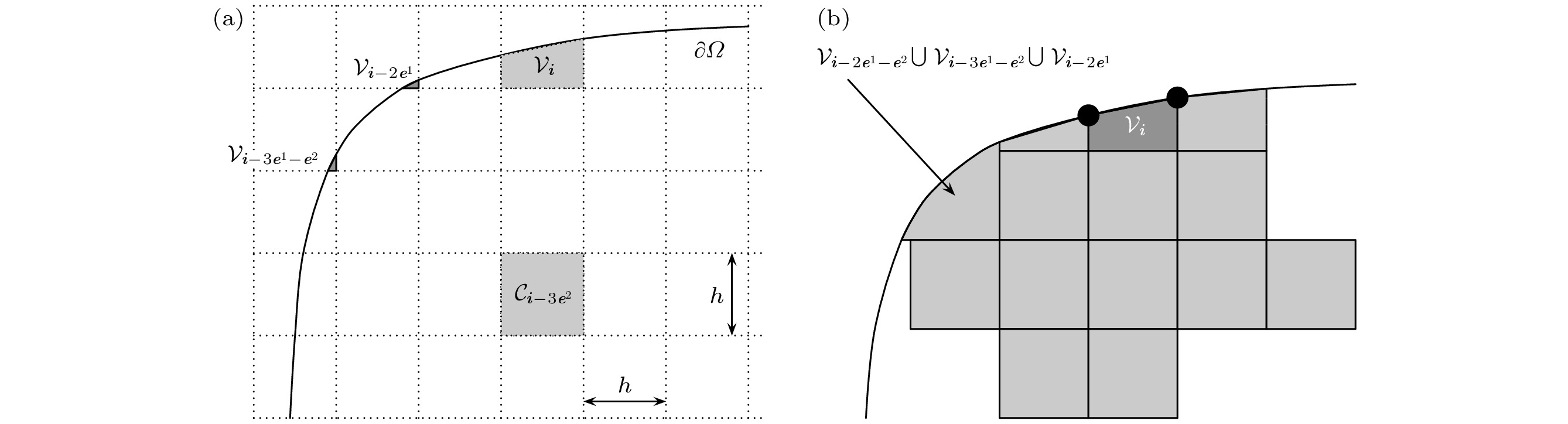 图 3 在不规则计算域上用正交网格离散Laplace算子
 图 4 从给定起始点开始选择一组格点以拟合多维n次完全多项式. 用拟合的完全多项式可以离散空间算子, 并且能很方便地满足边界条件[26]


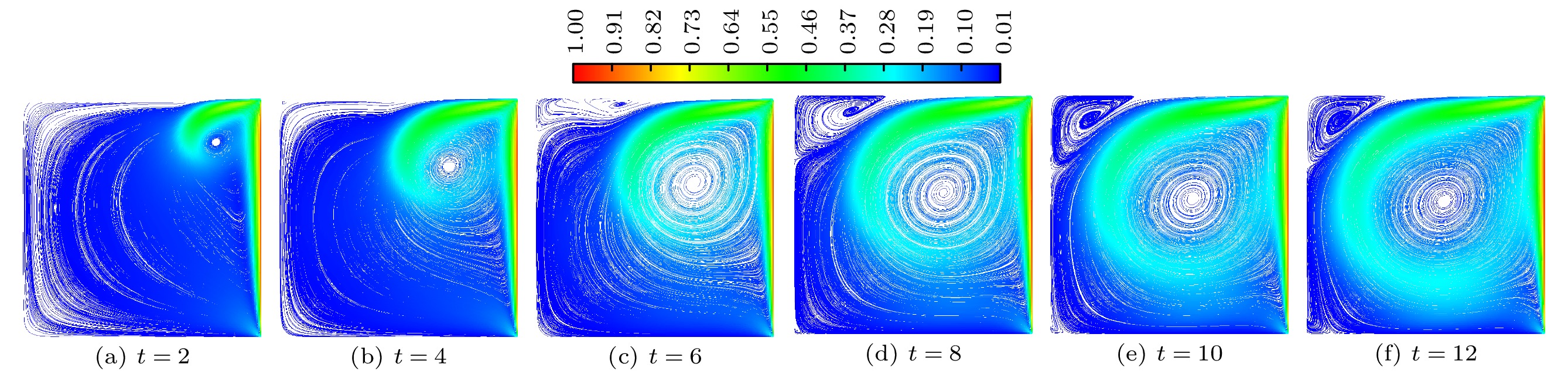 图 5 三维顶盖驱动方腔流测试中均匀网格上(


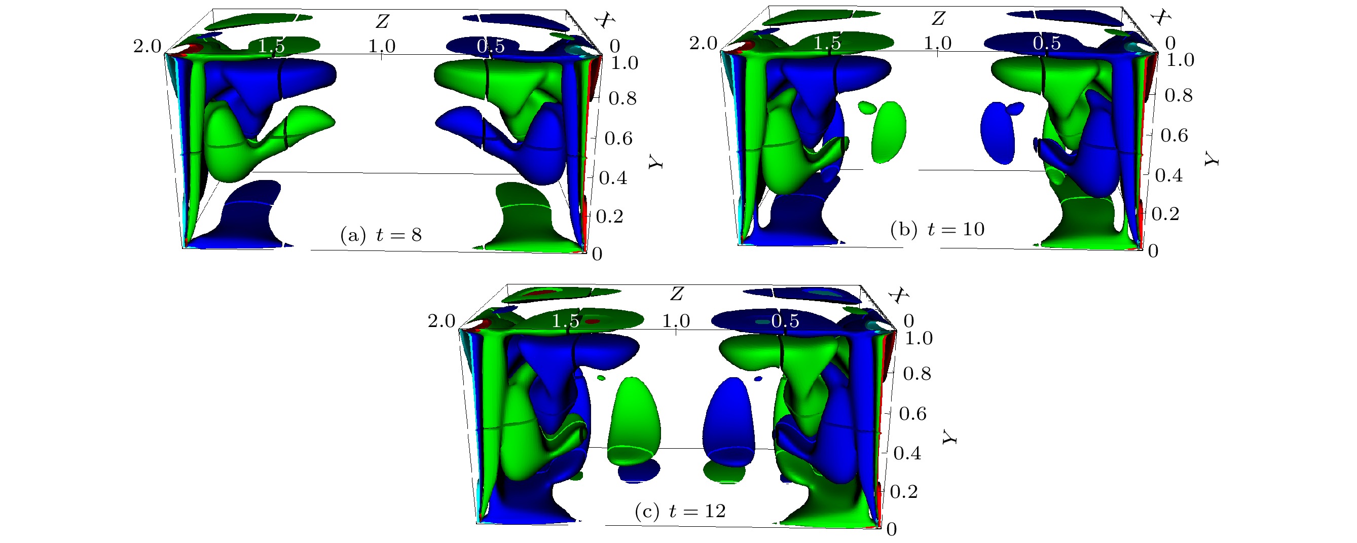 图 6 三维顶盖驱动方腔流测试中均匀网格上(


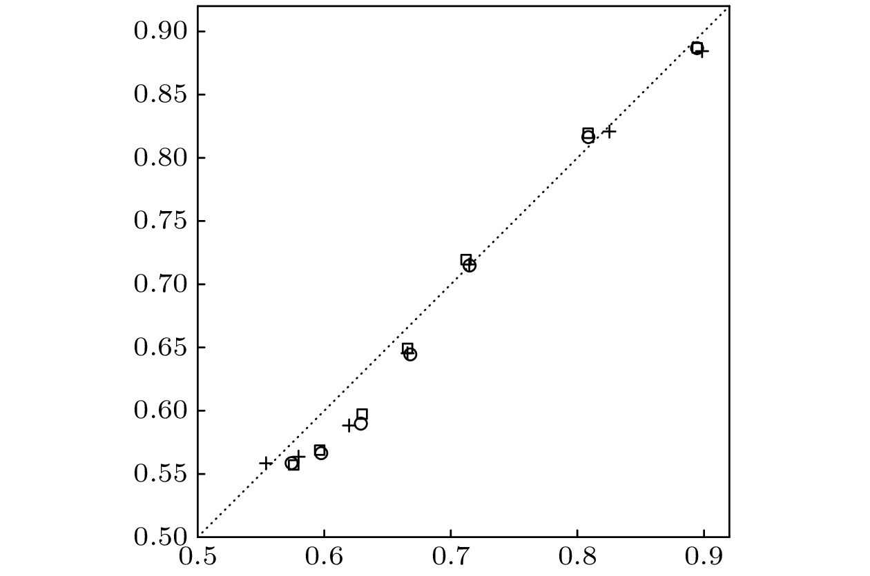 图 7 时刻


 图 8 三维顶盖驱动方腔流在时刻


 图 9 二维顶盖驱动方腔流测试中均匀网格上

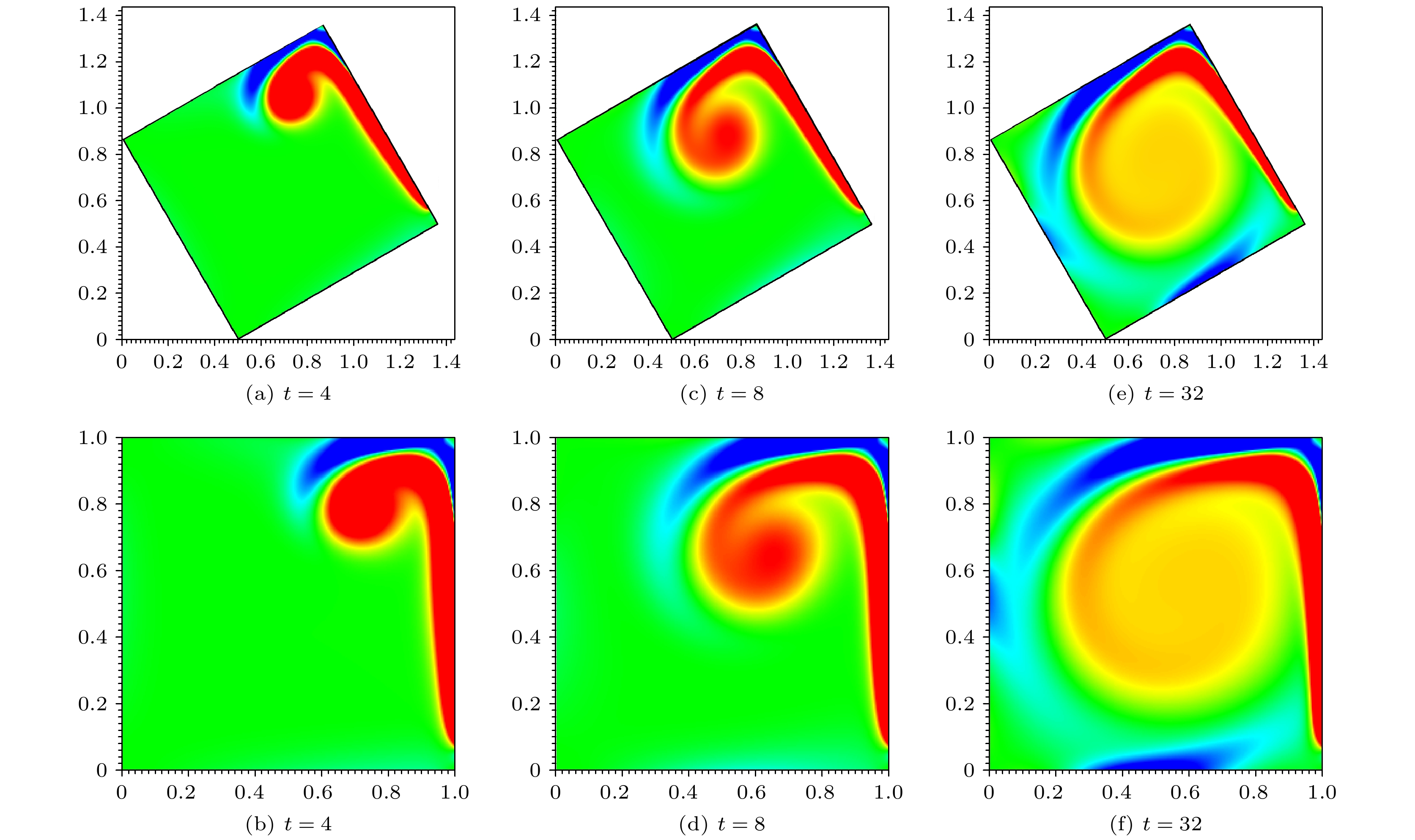 图 10 二维顶盖驱动方腔流测试中均匀网格上


