1.Key Laboratory for Laser Plasmas of Ministry of Education, School of Physics and Astronomy, Shanghai Jiao Tong University, Shanghai 200240, China 2.Tsung-Dao Lee Institute, Shanghai Jiao Tong University, Shanghai 200240, China
Fund Project:Project supported by the National Natural Science Foundation of China (Grant No. 11991074)
Received Date:08 December 2020
Accepted Date:22 January 2021
Available Online:26 June 2021
Published Online:05 July 2021
Abstract:Significant progress has been made in the studies of wakefield excitation in plasma by a self-modulated high energy proton beam in the past decade. The electron beams accelerated up to 2 GeV by using such a wakefield were demonstrated in the AWAKE experiment at CERN in 2018. Aiming at the application of high energy particle accelerators, new ideas have been investigated in recent years, such as seeding the proton beam self-modulation with an electron beam in order to enhance the strength and stability of the wakefield or adding a density transition in the plasma distribution to enhance the phase velocity and the strength of the wakefield. Here in this work, we investigate the effects of electron beam seeding on the phase velocity of the wakefield generated by the modulated proton beam in plasma. The physical mechanisms responsible for the phase velocity change and the roles played by the electron beam seeding are discussed. The theoretical analysis and two-dimensional particle-in-cell simulations show that both the growth rate and the phase velocity of the wakefield generated by the modulated proton beam can be enhanced by the electron beam seeding. The higher the charge density of the electron beam, the more significant the enhancement effects. The effects of electron beam energy and proton beam longitudinal profiles on the increase of phase velocity are also studied. It is shown that the evolution of the electron beam distribution has a significant effect on the seeding self-modulation process, and thus affecting the phase velocity. A self-focusing electron seeding beam can increase the phase velocity of the wakefield even to superluminal while an expanding seeding beam can reduce the phase velocity and destroy the stability of the whole process. This work may benefit the proton beam seeding self-modulation acceleration and its applications. Keywords:plasma wakefield acceleration/ self-modulation of proton beams/ wakefield phase velocity/ electron beam seeding
上述的计算使用了一个假设, 由于$ {r}_{0} $必然是个不为负的实数, 当$1-2 N\sin\left(\xi - {{\xi }_{1}}/{2}\right)\sin\left(-{\xi }_{1}\right)$为一个负数时, 直接假定$ 1/{r}_{0}=0 $, 另外, 在N的取值非常大的情况下, 比如N = 40, 此时电子束产生的电场已经处于非线性强度, 而本理论只适用于线性阶段, 所以上述的理论其实对于N有一个适用范围. 接着通过LCODE程序模拟理想状态下, 相同分布、不同电荷量的电子束所引发的种子自调制中不同位置、不同时刻纵向尾波极值的位置变化. LCODE是由Lotov开发的二维柱坐标模拟软件[25], 专门用于模拟柱对称粒子束在等离子体中传播所引起的尾波激发和电子加速过程. 在模拟中, 选取的模拟窗口长度为${600\; c/\omega }_{\mathrm{p}} $, 等离子体的密度为$ {n}_{0}=7\times {10}^{14}/\mathrm{c}{\mathrm{m}}^{3} $且均匀分布, 质子束长度$L= $$ 1500\; c/\omega _{\mathrm{p}}$(~3 cm), 半径$ {{r}_{\mathrm{b}}=1 c/\omega }_{\mathrm{p}} $(~200 μm), 中 心能量$ {E}_{\mathrm{b}}=400\;\mathrm{G}\mathrm{e}\mathrm{V} $, 中心密度为$ {n}_{\mathrm{b}}=0.0056\;{n}_{0} $, 纵向密度为均匀分布, 横向为高斯分布. 所使用的电子束中心密度为$ {n}_{\mathrm{b}\mathrm{e}} $, 纵向均匀分布, 横向为高斯分布, 电子束长度${{\xi }_{1}=\dfrac{\mathrm{\pi }}{2} c/}\omega _{\mathrm{p}}$, 半径$ {{r}_{\mathrm{b}\mathrm{e}}=1\; c/\omega }_{\mathrm{p}} $, 紧跟在质子束后方, 双方之间没有间隔. 这里先考虑一个理想情况, 把电子的能量设置为${E}_{\mathrm{b}\mathrm{e}}= $$ {10}^{15}\;\mathrm{G}\mathrm{e}\mathrm{V}$, 在能量如此高的情况下, 电子的分布不会随时间演化, 如此就可以与上述的理论进行比较. 图2(b)、图2(d)和图2(f)分别给出了在上述条件下改变电子束的中心密度所模拟出的质子束自调制尾波相速度在时间与空间上的分布. 而图2(a)、图2(c)和图2(e)给出了上述条件下质子束自调制尾波电场最大值在时间与空间上的分布. 通过对比这些图像可以发现, 随着电子束中心密度的增加, 电场最大值峰值出现的时间在整个自调制的过程中越来越早(从无电子束的大约$20000c/{\omega }_{\mathrm{p}}$到$ {n}_{\mathrm{b}\mathrm{e}}=10{n}_{\mathrm{b}} $时的大约$10000c/{\omega }_{\mathrm{p}}$), 相对应的尾波相速度变化结构也有着同样的变化, 由此可见, 电子束的引入可以提高自调制的增长率, 压缩整个自调制过程从初始到饱和所需的时间, 并且随着电子束的电荷量的增加, 整个加速的程度愈发明显. 图 2 电子束种子自调制模拟结果 (a) 无电子束时的最大电场分布; (b) 无电子束时的相速度分布; (c) 电子束中心密度为$ 1{n}_{\mathrm{b}} $时的最大电场分布; (b) 电子束中心密度为$ 1{n}_{\mathrm{b}} $时的相速度分布; (e) 电子束中心密度为$ 10{n}_{\mathrm{b}} $时的最大电场分布; (f) 电子束中心密度为$ 10{n}_{\mathrm{b}} $时的相速度分布 Figure2. Results of the simulation: (a) Distribution of Emax when no seeding; (b) distribution of phase velocity when no seeding; (c) distribution of Emax when $ {n}_{\mathrm{b}\mathrm{e}}=1{n}_{\mathrm{b}} $; (d) distribution of phase velocity when $ {n}_{\mathrm{b}\mathrm{e}}=1{n}_{\mathrm{b}} $; (e) distribution of Emax when $ {n}_{\mathrm{b}\mathrm{e}}=10{n}_{\mathrm{b}} $; (f) distribution of phase velocity when $ {n}_{\mathrm{b}\mathrm{e}}=10{n}_{\mathrm{b}} $.
图3(a)给出了在不同电子束条件下尾波的峰值相位变化情况. 通过对比图3(a)中的各个曲线的转折点位置, 可以发现所有的曲线都拥有相同的变化规律, 它们的变化趋势也是相同的, 惟一不同的是相速度拐点的位置和相速度的大小. 图3(b)和图3(c)则给出了($\xi =100\; c/{\omega }_{\mathrm{p}} $与$\xi =300\; c/{\omega }_{\mathrm{p}} $处)不同$ {n}_{\mathrm{b}\mathrm{e}} $下各处尾波相速度随时间的变化情况. 通过对比图3(b)和图3(c)不同$ {n}_{\mathrm{b}\mathrm{e}} $情况下的尾波相速度可以发现, 相比于无电子束调制, 在有电子束调制的情况下, 尾波相速度有所提升, 而且尾波的增长率也明显增加了. 质子束自调制的增长率随着电子束中心密度$ {n}_{\mathrm{b}\mathrm{e}} $的提高而增大, 从而缩短了整个过程的时间, 使得尾波相速度的演化进展加快, 更早地达到了后期相速度接近于光速的稳定状态. 这与之前理论推导所给出的结论完全一致, 但是可以发现模拟结果与理论相比在细节上并不一致, 可见想要获得一个精确的关于相速度的分布, 数值模拟仍然是不可或缺的. 图 3 (a) 不同电子束密度$ {n}_{\mathrm{b}\mathrm{e}} $情况下尾波峰值相位的变化; (b) $ \xi =100\; c/{\omega }_{\mathrm{p}} $处不同$ {n}_{\mathrm{b}\mathrm{e}} $条件下模拟得到的尾波相速度随时间变化; (c) $ \xi =300\; c/{\omega }_{\mathrm{p}} $处不同$ {n}_{\mathrm{b}\mathrm{e}} $条件下模拟得到的尾波相速度随时间变化 Figure3. (a) Phase change of the wakefield peak with different electron beam density $ {n}_{\mathrm{b}\mathrm{e}} $; (b) evolution of the phase velocity at $ \xi =100 c/{\omega }_{\mathrm{p}} $ with different $ {n}_{\mathrm{b}\mathrm{e}} $; (c) evolution of the phase velocity at $ \xi =300 c/{\omega }_{\mathrm{p}} $ with different $ {n}_{\mathrm{b}\mathrm{e}} $.
图4给出了纵向坐标$0 c/{\omega }_{\mathrm{p}}—600 c/{\omega }_{\mathrm{p}} $范围的模拟窗口内纵向电场最大值随时间的变化曲线, 从图中的曲线变化可以清晰地看出随着电子束的电荷量提升, 整个自调制过程的增长率(电场增长率)有了明显的提升, 所达到的最大电场也随之提高. 图 4 不同电子束密度$ {n}_{\mathrm{b}\mathrm{e}} $情况下最大电场随时间的分布 Figure4. Evolution of the maximum electric field with different electron beam density $ {n}_{\mathrm{b}\mathrm{e}} $.
接下来的模拟是基于之前的等离子体和质子束参数, 考虑了相同电子束分布和电荷量, 但不同能量的模拟参数对尾波相速度的影响. 在模拟中, 等离子体的密度为$ {n}_{0}=7\times {10}^{14}/\mathrm{c}{\mathrm{m}}^{3} $且均匀分布, 质子束中心能量$ {E}_{\mathrm{b}}=400~\mathrm{G}\mathrm{e}\mathrm{V} $, 长度$ {L=1500 c/\omega }_{\mathrm{p}} $(大约3 cm), 半径$ {r=1 c/\omega }_{\mathrm{p}} $(大约200 μm), 中心密度为$ {n}_{\mathrm{b}\mathrm{m}}=0.0056{n}_{0} $, 纵向分布为均匀分布, 横向为高斯分布. 所使用的电子束长度${{\xi }_{1}=\dfrac{\mathrm{\pi }}{2} c/\omega }_{\mathrm{p}}$, 半径$ {r=1 c/\omega }_{\mathrm{p}} $, 电子束中心密度$ {n}_{\mathrm{b}\mathrm{e}\mathrm{m}}=10{n}_{\mathrm{b}} $, 纵向分布为均匀分布, 横向为高斯分布, 电子束中心能量总共选取了三种, 分别是$ {E}_{\mathrm{b}\mathrm{e}}$ = 100 MeV, 500 MeV, 1 GeV. 图7(a)—图7(c)给出了在上述条件下改变电子束的能量(100 MeV, 500 MeV, 1 GeV)所得到的质子束自调制尾波电场最大值在时间与空间上的分布. 图7(d)�—图7(f)则给出了上述条件下质子束自调制尾波相速度在时间与空间上的分布. 图8(a)和图8(b)则是挑选了$\xi =100 c/{\omega }_{\mathrm{p}}$与$\xi = $$ 300 c/{\omega }_{\mathrm{p}}$的位置, 不同能量的电子束所得到的尾波相速度进行比较. 可以发现, 在自调制初始的时期, 出现了相速度大于光速的现象, 这与之前提到的电子束自聚焦理论相符合. 能量越高, 该现象就越不明显. 另外通过对比图7和图8中的数据, 可以发现对自聚焦起到关键作用的有两个参数, 即电子束的能量和密度. 如果电子束的能量γ过高, 那么它受到的径向加速度也随之减弱, 如图8(a)和图8(b)所示, 自聚焦对相速度的影响程度随着能量的增高而渐渐减弱. 而如果增强电子束的密度, 则自聚焦的速度就会明显加快, 整个自聚焦的过程所引发的超光速相速度也会愈发明显. 图 7 利用电子束种子尾波调制质子束的模拟结果 (a), (b), (c)分别对应电子束能量$ {E}_{\mathrm{b}\mathrm{e}} $ = 100 MeV, 500 MeV, 1 GeV时的最大电场随时间变化; (d), (e), (f) 分别对应电子束能量$ {E}_{\mathrm{b}\mathrm{e}} $ = 100 MeV, 500 MeV, 1 GeV时的相速度随时间变化 Figure7. Simulation of proton beam modulation with electron beam seeding:(a), (b), (c) The maximum electric fields as a function of time for the electron beam energy at ${E}_{\mathrm{b}\mathrm{e}}=100~\mathrm{M}\mathrm{e}\mathrm{V}$, 500 MeV, and 1 GeV, respectively; (d), (e), (f) the phase velocity as a function of time for the electron beam energy at ${E}_{\mathrm{b}\mathrm{e}}=100~\mathrm{M}\mathrm{e}\mathrm{V}$, 500 MeV, and 1 GeV, respectively.
图 8 (a) 在$ \xi =100 c/{\omega }_{\mathrm{p}} $处不同电子束能量模拟得到的尾波相速度随时间变化; (b) 在$ \xi =300 c/{\omega }_{\mathrm{p}} $处不同电子束能量模拟得到的尾波相速度随时间变化 Figure8. (a) Phase velocity as a function of time at $ \xi =100 c/{\omega }_{\mathrm{p}} $ for different electron energy; (b) phase velocity as a function of time at $ \xi =300 c/{\omega }_{\mathrm{p}} $ for different electron energy.


 图 1 在
图 1 在


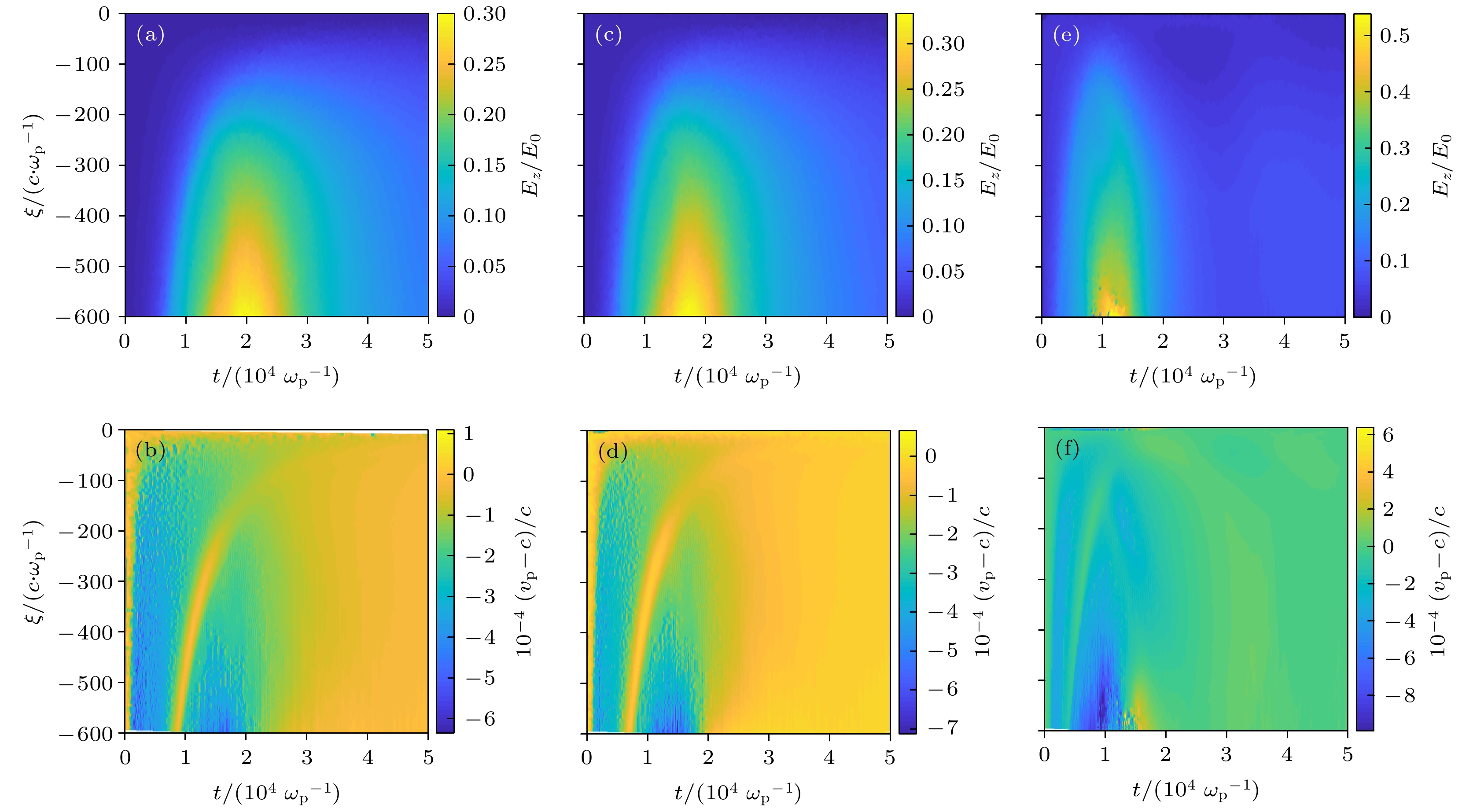 图 2 电子束种子自调制模拟结果 (a) 无电子束时的最大电场分布; (b) 无电子束时的相速度分布; (c) 电子束中心密度为


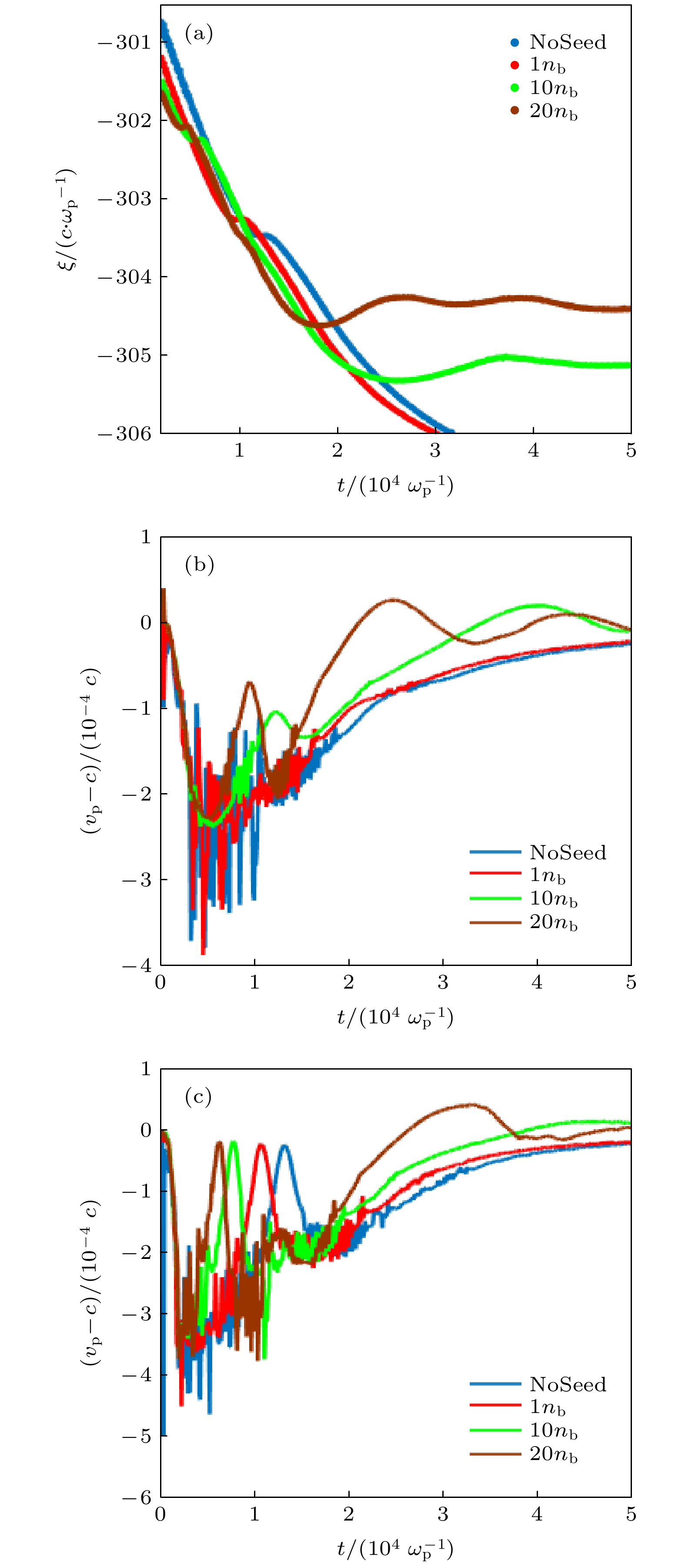 图 3 (a) 不同电子束密度


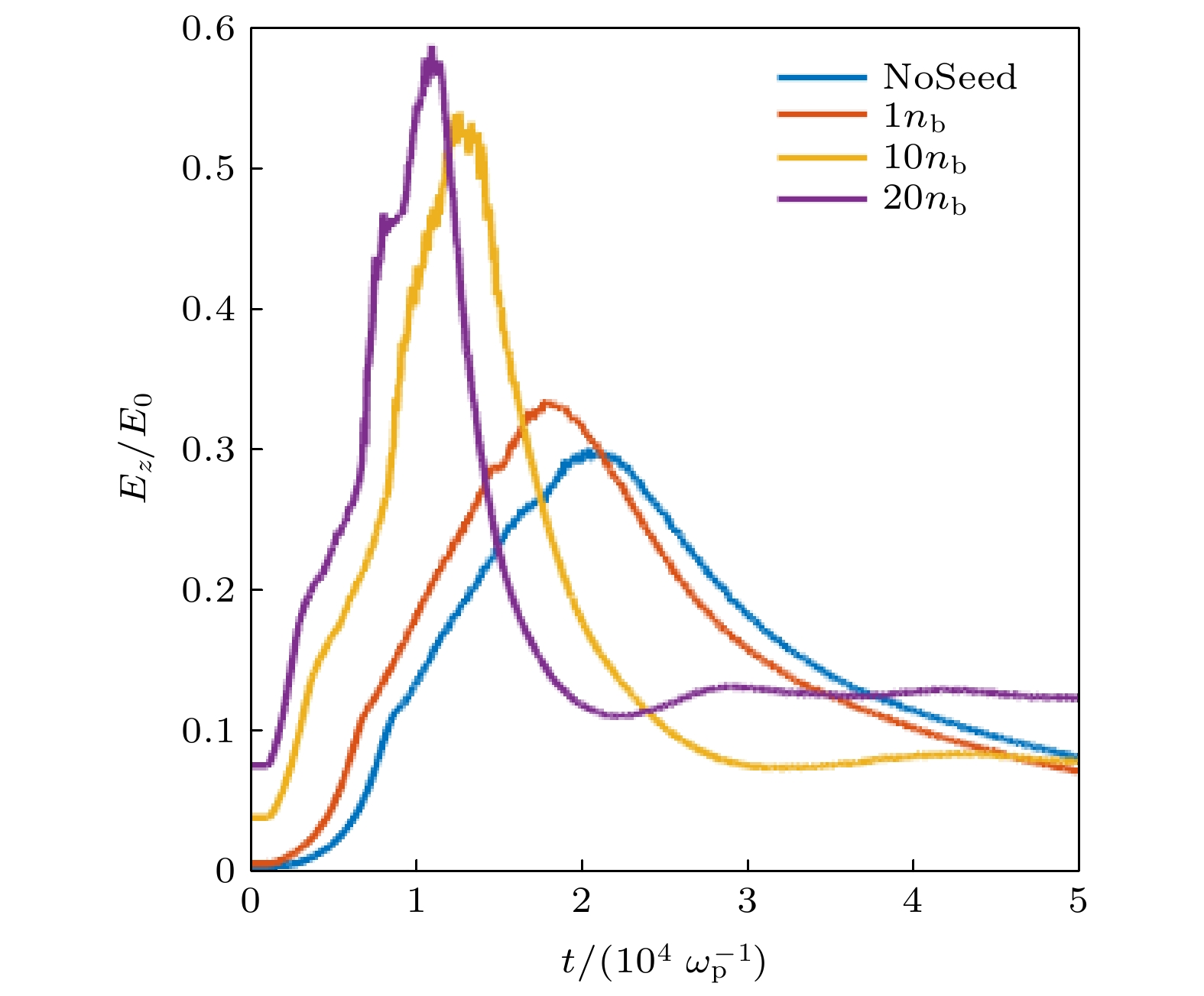 图 4 不同电子束密度


 图 5 (a) 电子束能量


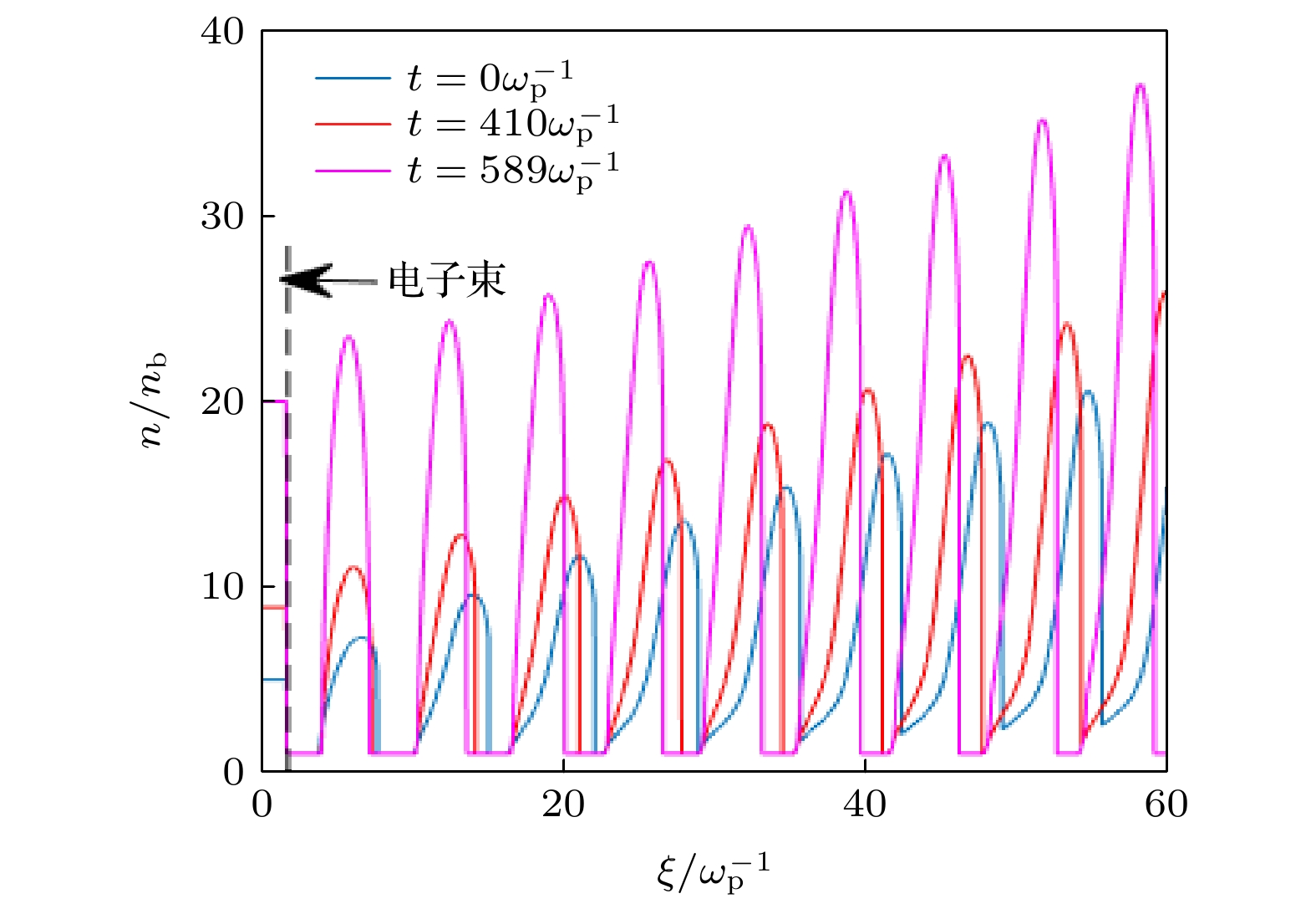 图 6 电子束压缩引起的质子束平衡态变化, 即在三个时刻的质子束平衡态分布


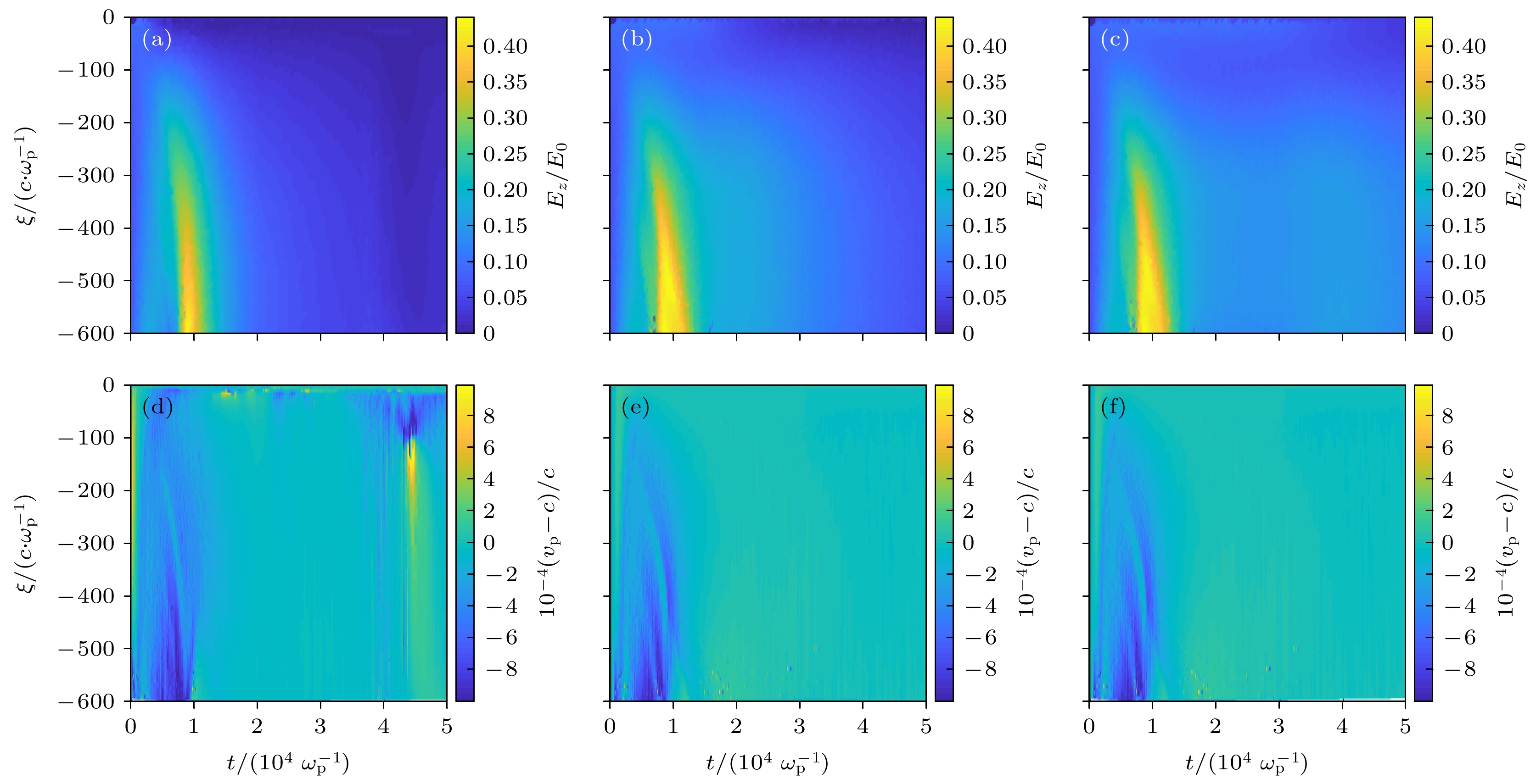 图 7 利用电子束种子尾波调制质子束的模拟结果 (a), (b), (c)分别对应电子束能量


 图 8 (a) 在


 图 9 (a) 在