Abstract:Proton radiography is a widely used method to diagnose the electromagnetic field of plasma. When protons pass through the electromagnetic field of plasma, they are deflected by Lorentz force and redistributed on the recorder. How to reconstruct electromagnetic field from the experimental result is an open problem. In this paper, we take the laser-driven capacitor-coil target for example to introduce and compare particle tracing and flux analysis, which are two widely used methods in proton radiography experiment to reconstruct the magnetic field. The capacitor-coil target is an important method to generate strong magnetic field in laser plasma experiment, where the strong current flows in the coil and its producing magnetic field may be larger than kilotesla. Firstly, the theoretical magnetic fields of capacitor-coil target are calculated with current being 10 kA and 50 kA. Secondly, the Geant4 is used to simulate the proton radiographs, where protons with 7.5 MeV pass through the target and the theoretical magnetic field is recorded. Thirdly, the theoretical proton radiographs are analyzed by the flux analysis method, and two magnetic fields are reconstructed. Finally, the theoretical magnetic fields are compared with the reconstructed ones, and the advantages and disadvantages of these two methods are analyzed. Particle tracing rebuilds the geometry distribution of proton source, plasma magnetic field and recorder in experiment, and it needs few assumptions. However, it strongly relies on accurate calculation of theoretical magnetic field and proton trajectory, and it requires to change the magnetic field over and over to achieve a closest result to the experimental proton radiograph. Meanwhile, particle tracing method consumes a lot of computation sources. The flux analysis directly reconstructs the magnetic field from experimental proton radiograph. However, it is only applicable to the case of weak magnetic field, and the error becomes larger for the case of stronger magnetic field. A dimensionless parameter μ is used to estimate the deflection of proton in the magnetic field, which measures the amount of deflection per unit length in the interaction region. The flux analysis method is applicable to the $\mu\ll 1$ regime. Additionally, the target may absorb the proton when the energy of proton is low and produces shadow on the proton radiograph, which leads to some difference between the original magnetic field and the reconstructed result. Keywords:proton radiography/ laser plasma/ generation of magnetic field/ diagnostic technique
全文HTML
--> --> --> 1.引 言质子背光成像技术(proton radiography)是一个被广泛应用于高能量密度物理研究领域的诊断等离子体电磁场结构的诊断手段[1-3]. 因为等离子体电磁场的存在, 从点源出射的质子穿过等离子体, 受洛伦兹力(Lorentz force)偏折在等离子体后的成像板上形成一定的流量分布. 通过分析质子的分布便能反推出所经过的电磁场分布和强度等物理信息. 这种诊断手段已经被广泛应用于与磁重联[3]、惯性约束聚变[4]、无碰撞冲击波[5]、不稳定性[6]等相关的高能量密度物理实验中. 质子背光成像诊断技术首先需要产生质子点源, 现在主要有两种手段. 第一种依靠短脉冲激光($>\! 10^{18}$ W/cm2)聚焦到薄膜靶上利用靶后法向鞘场(target normal sheath field)加速形成质子源[7-11]. 薄膜靶一般使用金膜, 所产生质子的能量为连续谱, 实验中所用能量范围大约为3—60 MeV. 一般这种质子成像方式用RCF(remote call framework)堆栈(radiochromic film stack)记录成像结果, 由于每层RCF对质子的阻止本领(stopping power)不同, 可以认为每层RCF对应不同能量的质子穿过电磁场的结果. 第二种使用多束激光聚焦到充满D3He的内爆靶通过核反应D + D → T + p和D + 3He $ \rightarrow \alpha $ + p 产生[12,13], 这两个反应分别能够产生质子能量为3 MeV和14.7 MeV 的两个展宽很窄的单能峰, 使用这样的质子能够得到比较清晰的质子成像结果[4]. 当等离子体的密度范围在$ 10^{16}—10^{20} $ cm–3之间时, 质子穿过等离子体时的碰撞散射作用可以忽略不计[14]. 例如10 MeV 的质子束穿过密度为1020 cm–3长度为1 mm的碳等离子体, 只损耗0.1%的质子能量. 相对于使用电子束测量等离子体的电磁场, 可测量的密度上限更高[15]. 此外, 质子背光成像技术的空间分辨能力能够达到几微米, 同时时间分辨能力为1—10 ps. 因此质子成像技术是一个很有效的等离子体诊断手段[16-18]. 但是由于实验和分析手段的限制, 怎样有效地分析质子成像结果并从中提取更多更准确的物理信息仍然是一个开放性课题[16-18]. 由于等离子体中复杂的三维电磁场结构, 实验中所获得的质子成像结果一般很难与电磁场形成简单的一一对应的关系. 现在通过质子成像结果重构等离子体电磁场的方法大致可以分为两种. 一种是粒子追踪法(particle tracing), 通过在理论模型中重构实验设置, 将质子源、等离子体和成像板按实验中的位置放置, 进而得到质子成像的理论模拟结果. 通过对比模拟结果和实验结果, 最后揭示等离子体中的电磁场结构. 另一种是流量分析法(flux analysis), 通过分析实验质子成像结果的流量分布而得到电磁场对质子的偏折信息, 进而反演出质子通过区域的电磁场结构. 这两种方法广泛应用于实验分析中, Li 等[3]使用粒子追踪法将用LASNEX 计算得到的磁场代入到混合PIC (particle in cell)程序LSP中, 模拟了用质子背光技术测量激光等离子体电磁场的实验. Du等[19,20] 使用粒子追踪法研究发现韦伯不稳定性(Weibel instability)中电场对质子偏折大于磁场, 并用流量分析法重构反演得到电场的强度. 本文以电容线圈靶(capacitor coil)的磁场为例来对比两种磁场反演的方法. 使用激光驱动电容线圈靶产生磁场首先由Daido等[21]在1986年提出. 电容线圈靶如图1(a)中所示, 该种靶由两片平行的靶盘和一个连接的细丝组成, 其中一个靶盘有一个注入孔. 高功率激光从注入孔进入聚焦在另外一个靶盘上, 产生超热电子离开该盘, 进而两盘之间产生很强的电势差, 在细丝上生成电流, 最后得到感应磁场. 图1(b)展示了电容线圈靶的电流方向和相应的磁场分布. 最初在VULCAN激光装置上的实验利用该种靶型得到了几特斯拉的磁场[22], 后来Fujioka等[23]在GEKKO-XII激光装置上得到了峰值大约1.5 kT的强磁场. 现在这种靶型被运用于磁重联等与强磁场相关的实验中[24,25]. 根据以前相关工作, 电容线圈靶主要靠电流产生很强的磁场, 本文中只讨论磁场结构对质子的偏折, 暂不讨论电场的影响. 从理论方面对比两种方法, 讨论这两种方法的适用性和对以后实验可提供的参考. 本文的思路是: 首先计算电容线圈靶在给定电流强度下的磁场, 然后用粒子追踪的方法计算质子照相的图片代替实验结果, 再用流量分析法反演这幅图片重构磁场, 最后比较重构的磁场与原来理论磁场的不同. 图 1 (a)电容线圈靶构造; (b)电容线圈靶磁场的分布示意图, 粉红色半透明区域为靶结构, 白色箭头标示了电流方向, 彩色箭头为X-Y平面的磁场结构; (c) 质子成像技术实验设置 Figure1. (a) Configuration of capacitor-coil target; (b) schematic of magnetic field of capacitor-coil target. Pink-semitransparent is the coil, white arrows indicate the current direction, and colorful arrows indicate the magnetic field in X-Y plane; (c) experimental setup of proton radiography.
3.结果与讨论Geant4计算的质子经过不同磁场后的质子成像结果如图2所示. 图2(a)给出了在没有磁场时, 质子穿过作用区域在成像板上得到的电容线圈靶的正面静态图(阴影). 从质子传输的方向看去, 两个圆形的盘重叠遮挡质子, 在图片上部形成圆形的质子较少的区域; 下垂的线圈的直线和圆弧部分重叠, 在成像板上则只剩下一个细长的矩形区域(红色虚线区域). 这是因为Ni元素对7.5 MeV质子的阻止本领大约为为$ 3.62\!\times\!10^{-21} $ MeV·cm2, 则质子穿过数密度大约为9$ \times10^{22} $ cm–3的重叠的两层固体靶盘(300 μm)后会被完全吸收[29]. 而实验中靶之外区域Ni等离子体的密度[24,25]小于1020 cm–3, 对质子的影响可以忽略, 可以用来诊断这些区域的磁场结构. 图 2 Geant4模拟结果, 图片中的坐标为放大10倍的成像板处的坐标 (a)线圈电流I = 0的静态结果; (b)线圈电流I = 10 kA的结果; (c)线圈电流I = 50 kA的结果. 红色虚线是线圈阴影的位置 Figure2. Simulation results of Geant4, the coordinates are adjusted at the position of detector: (a) Coil current I = 0; (b) coil current I = 10 kA; (c) coil current I = 50 kA. The red dash regions are the position of the shadow of the coils
使用$ I_1 $ = 10 kA 和$ I_2 $ = 50 kA两个电流强度, 相应的沿质子传输路径积分的磁场结构和强度分布的理论值展示于图3中. 当电容线圈通过电流, 产生的磁场呈同心圆状围绕在线圈周围, 随着距离的增加而衰减. 图2 (b)和图2(c)展示了在两个磁感应强度下Geant4 计算的质子成像结果. 根据无电场的洛伦兹力$ { F} = e{ v}\times\; { B} $, 当质子穿过围绕线圈顶端的环状磁场, 质子将被向中间区域聚集. 由于磁场增强, 50 kA 的情况比10 kA 的情况中质子的聚集效应更加明显. 除了质子被聚集到线圈顶端区域, 由于磁场的三维结构还形成了一些细微的结构. 图 3 (a) I = 10 kA的理论磁场结构分布; (b) I = 50 kA 的理论磁场结构分布; (c) I = 10 kA 的理论磁感应强度分布; (d) I = 50 kA的理论磁感应强度分布. 黑色虚线是线圈阴影的位置. 图片中的坐标为放大10 倍后成像板处的坐标 Figure3. (a) Theoretical magnetic strength for I = 10 kA; (b) theoretical magnetic strength for I = 50 kA; (c) theoretical magnetic configuration for I = 10 kA; (d) theoretical magnetic configuration for I = 50 kA. The black dash regions are the position of the shadow of the coils. The coordinates are adjusted at the position of detector
以图2(a)为静态图, 分别从图2(b)和图2(c)反演重构磁场, 质子成像结果和重构磁场都是1001 × 1001的二维矩阵, 质子能量7.5 MeV, 质子源到靶的距离1 cm, 靶到成像板的距离9 cm, 每个间隔对应20 μm. 图4给出了反演重构得到的两种电流强度下沿传输路径积分的磁感应强度和结构分布. 图5(a)和图5(b)展示了线圈遮挡区域及其沿Y 轴方向(–0.15 cm < X < 0.15 cm)的磁场平均值. 对比图3(b)和图4(b) 中的磁场结构, 类似于理论磁场, 重构的磁场结构也是围绕线圈顶端呈同心圆的结构. 但是对比图3 (d)和图4(d)中磁场的强度分布可以发现两者的不同, 这是因为流量分析法限制于基本假设, 只能通过较小范围内的质子分布重构磁场, 但是当磁场较强时, 较大范围内的质子都可能被折射到该区域. 即流量分析法会低估质子被偏折的距离而低估磁场强度. 也会因为只考虑较小范围内的质子偏折, 而造成较大范围内重构磁场和理论磁场强度分布的不同. 图5(a)和图5(b)中红线表示重构的磁场比较离散, 因此图4 中较难得到如图3中那样规则的等高线图. 图5(a)显示, I = 10 kA 的情况中, 在线圈的外部(Y < –0.45 cm)较好地重构了磁场的强度分布, 磁场围绕线圈顶端向远处衰减. 但是在线圈的遮挡区域(–0.15 cm < X < 0.15 cm, Y < –0.45 cm), 重构的磁场与理论磁场相差较大. 这是因为在质子成像中, 由于线圈的遮挡形成空白区域, 而实际线圈包围的内部区域磁场较强, 这造成了重构磁场和理论磁场在这个区域的不同. 但是当磁场较大(I = 50 kA)时, 重构磁场与理论磁场相差都比较大, 无论在线圈的环绕内部还是外部区域重构得到的磁场都远小于理论磁感应强度. 图 4 (a) I = 10 kA的理论重构结构分布; (b) I = 50 kA 的重构磁场结构分布; (c) I = 10 kA 的重构磁感应强度分布; (d) I = 50 kA的理论重构强度分布. 黑色虚线是线圈阴影的位置. 图片中的坐标为放大10 倍后成像板处的坐标 Figure4. (a) Reconstructed magnetic strength for I = 10 kA; (b) reconstructed magnetic strength for I = 50 kA; (c) reconstructed magnetic configuration for I = 10 kA; (d) reconstructed magnetic configuration for I = 50 kA. The black dash regions are the position of the shadow of the coils. The coordinates are adjusted at the position of detector
图 5 (a) I = 10 kA, 沿Y方向的理论磁场和重构磁场在–0.15 cm < X < 0.15 cm 区域平均值的对比; (b) I = 50 kA, 沿Y方向的理论磁场和重构磁场在–0.15 cm < X < 0.15 cm 区域平均值的对比. (a)和(b)中黑色实线是理论值, 红色实线是重构值, 黑色虚线是线圈顶端对应的位置; (c)两种情况下沿Y 方向μ值的对比, 蓝色实线为I = 10 kA的结果, 绿色实线为I = 50 kA 的结果 Figure5. (a) Comparison between the mean theoretical and the mean reconstructed magnetic field for the I = 10 kA case in the region of –0.15 cm < X < 0.15 cm along Y direction; (b) comparison between the mean theoretical and the mean reconstructed magnetic field for the I = 50 kA case in the region of –0.15 cm < X < 0.15 cm along Y direction. The black solid lines are the theoretical results. The red solid lines are the reconstructed line. The black dash lines are the position of the tips of the coils; (c) comparison of μ value along the Y direction between the I = 10 kA and I = 50 kA cases


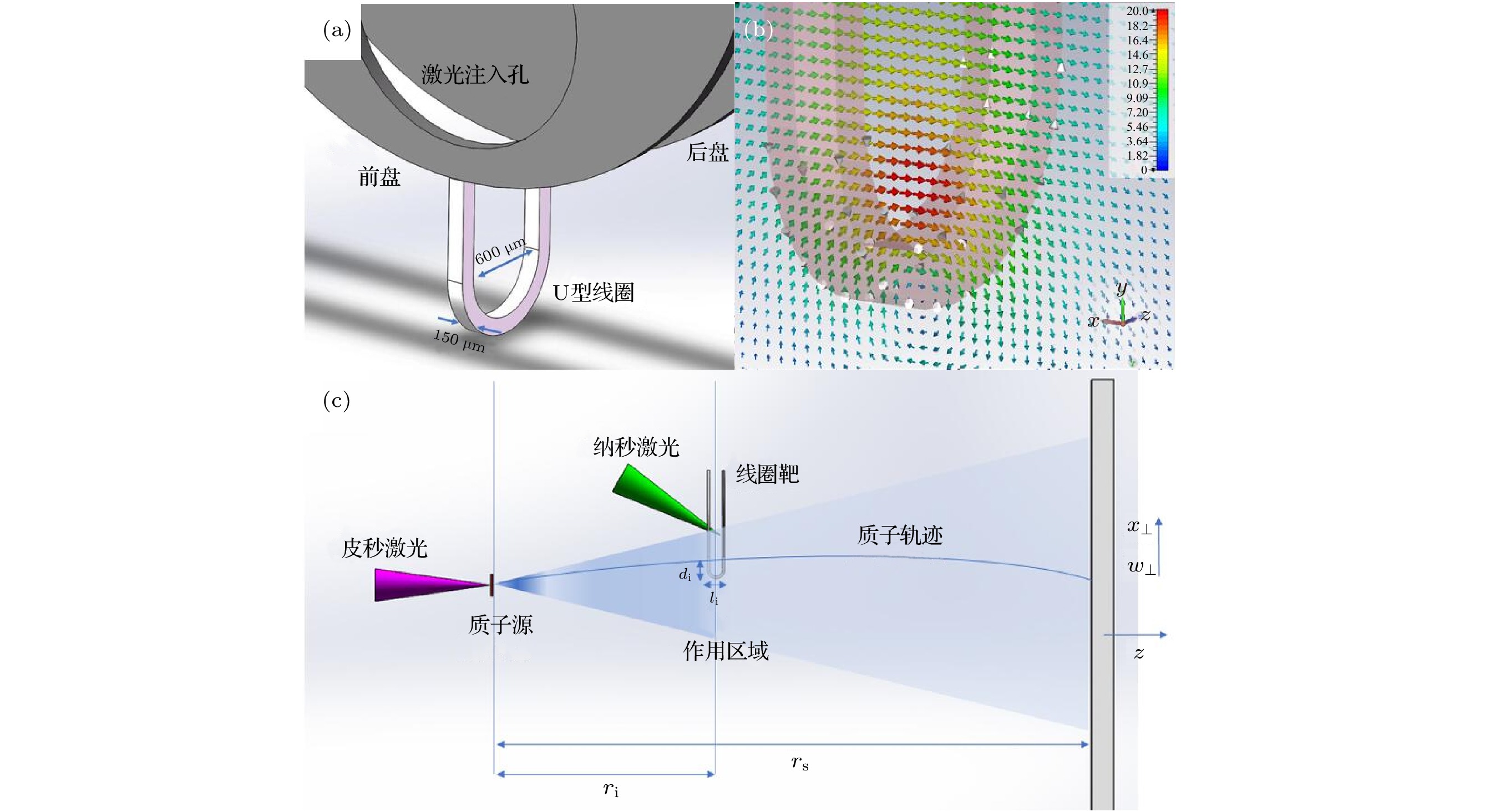 图 1 (a)电容线圈靶构造; (b)电容线圈靶磁场的分布示意图, 粉红色半透明区域为靶结构, 白色箭头标示了电流方向, 彩色箭头为X-Y平面的磁场结构; (c) 质子成像技术实验设置


 图 2 Geant4模拟结果, 图片中的坐标为放大10倍的成像板处的坐标 (a)线圈电流I = 0的静态结果; (b)线圈电流I = 10 kA的结果; (c)线圈电流I = 50 kA的结果. 红色虚线是线圈阴影的位置


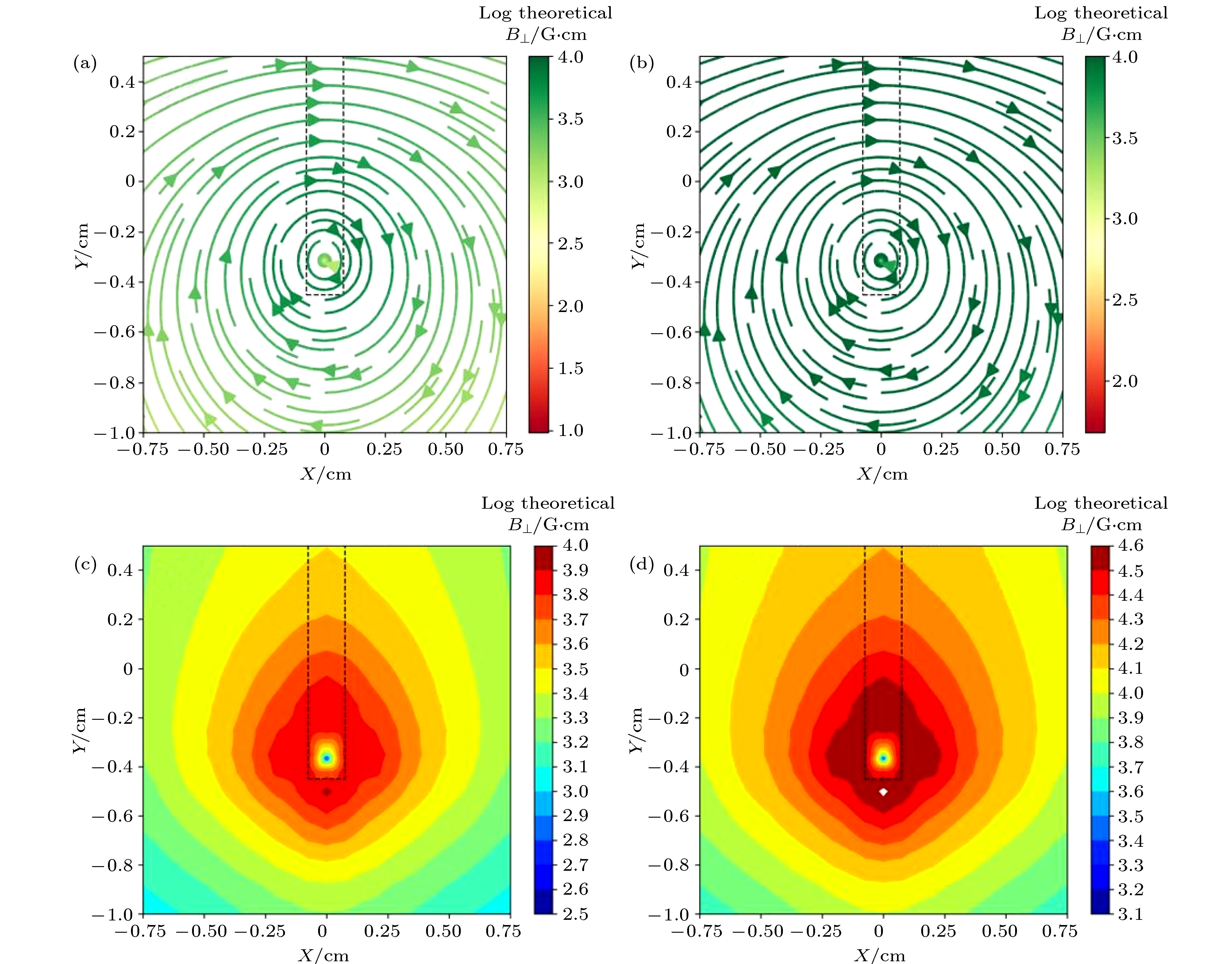 图 3 (a) I = 10 kA的理论磁场结构分布; (b) I = 50 kA 的理论磁场结构分布; (c) I = 10 kA 的理论磁感应强度分布; (d) I = 50 kA的理论磁感应强度分布. 黑色虚线是线圈阴影的位置. 图片中的坐标为放大10 倍后成像板处的坐标
 图 4 (a) I = 10 kA的理论重构结构分布; (b) I = 50 kA 的重构磁场结构分布; (c) I = 10 kA 的重构磁感应强度分布; (d) I = 50 kA的理论重构强度分布. 黑色虚线是线圈阴影的位置. 图片中的坐标为放大10 倍后成像板处的坐标
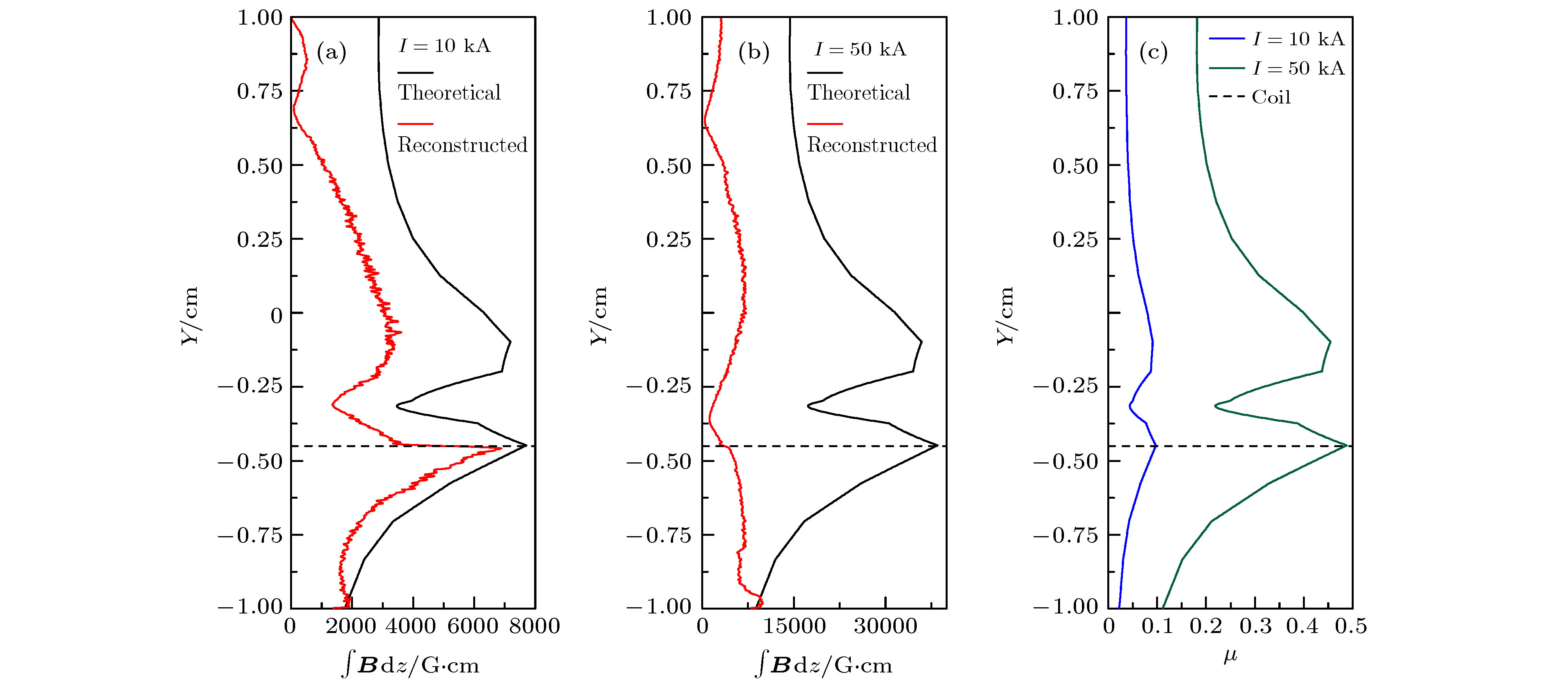 图 5 (a) I = 10 kA, 沿Y方向的理论磁场和重构磁场在–0.15 cm < X < 0.15 cm 区域平均值的对比; (b) I = 50 kA, 沿Y方向的理论磁场和重构磁场在–0.15 cm < X < 0.15 cm 区域平均值的对比. (a)和(b)中黑色实线是理论值, 红色实线是重构值, 黑色虚线是线圈顶端对应的位置; (c)两种情况下沿Y 方向μ值的对比, 蓝色实线为I = 10 kA的结果, 绿色实线为I = 50 kA 的结果


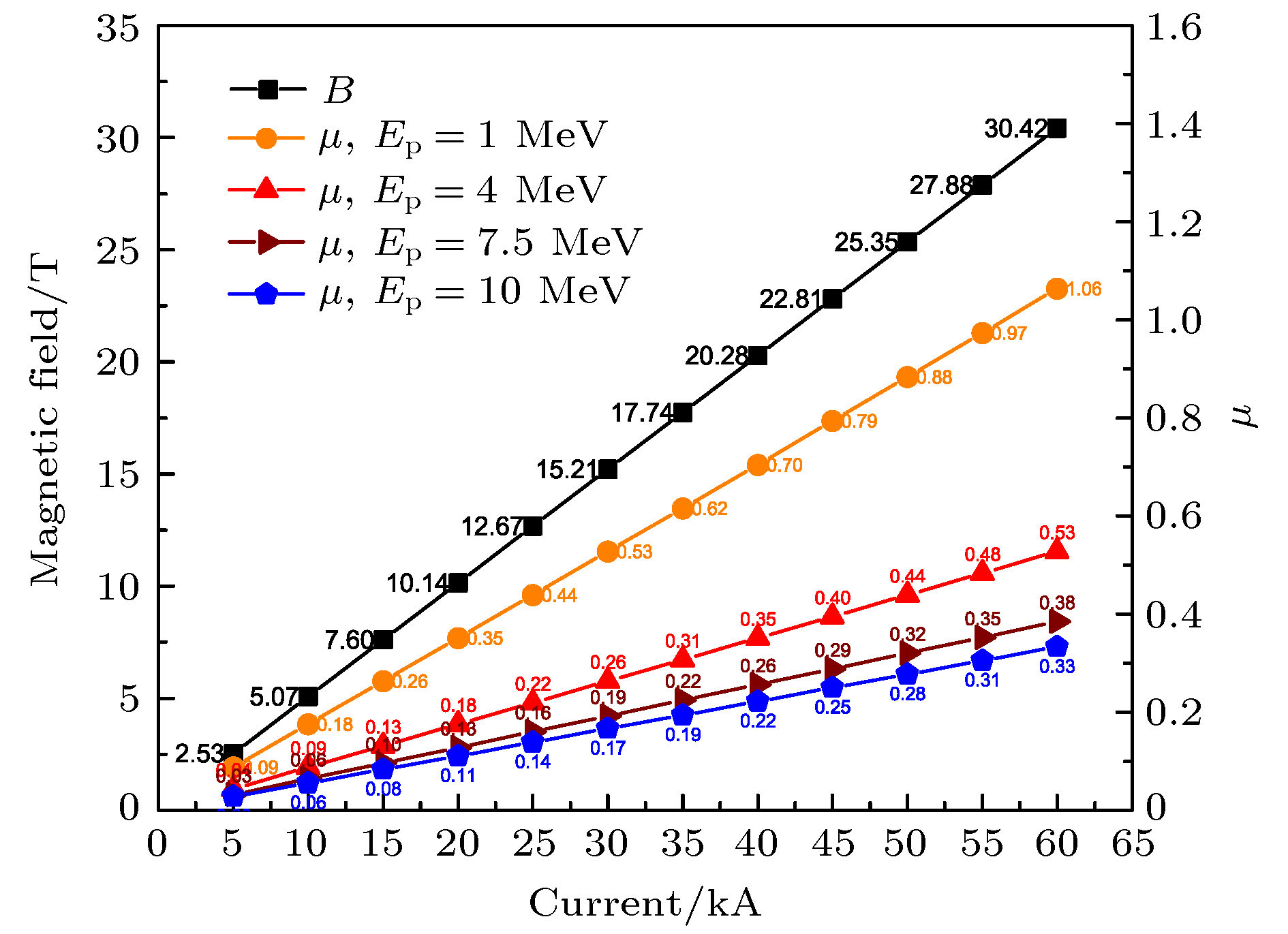 图 6 黑色实线和散点是电流强度与圆弧顶点处磁感应强度的关系. 不同颜色的实线和散点分别是质子能量为1, 4, 7.5 和10 MeV时实验设置中相应的μ值