Abstract:In this paper, we propose a new type of relativistic regional innovation index by using the international patent application data. Based on the super-linear relationship between regional innovation and economic development, the new index can eliminate the influence of economic development level on innovation capabilities, and can effectively achieve the comparison of innovation capabilities among economies at different economic development levels. This new index is quite simple, and points out a series of new findings that are sharply different from the traditional cognitive phenomena, e.g. the index shows that the technological innovation capabilities of mainland China are among the highest in the world in 1980s. Moreover, the use of this new index not only can efficiently explain the economic growth of countries in the world at a higher level, but also find that there is a novel 20-year business cycle in the correlation between the index and economic growth rate. These results show that the index, as a simple single indicator, can achieve a higher degree of explanatory ability with minimal data dependence. This new index not only repositions the innovation capacity of world’s economies, but also provides a new insight into an in-depth understanding of the relationship between innovation and economic development, and implies the development potential and application space such a kind of relativistic economic indicator. Keywords:regional innovation index/ business cycle/ relativistic economic indicator/ complexity in economy
其中$n_Y^{{i}}$为经济体i在年份Y的相对人均专利申请数, ${N_Y^{{i}}}$为经济体i在年份Y的人均专利申请数, 尖括号表示在年份Y的人均专利申请数的世界均值. 通过这两个相对性的人均指标, 世界各经济体在不同年份的人均GDP和人均专利数都被纳入了一个可有效比较的范畴中. 图1显示了各个经济体自1985年以来在由相对人均GDP的对数值g(例如对经济体i, 有gi = log10(Gi))和相对人均专利申请数的对数值np(对经济体i, 有npi = log10(ni))所构成的空间中的变化曲线. 可以看到, 发达经济体同发展中经济体之间有着较为明显的分离, 其分离区域大致如图1点划线所示. 中国大陆地区的曲线在g和np两者都呈现出稳定而快速的增长趋势, 而韩国是极少数已经实现了从发展中经济体区域向发达经济体区域大幅度跨越的经济体之一. 图 1 世界各经济体在由相对人均GDP的对数g和相对人均专利申请数的对数np(两者均以10为底数)所构成的空间中的变化轨迹. 彩色曲线为11个代表性经济体在该空间的轨迹, 灰色曲线为其他经济体. 灰色虚线为拟合直线np = 1.12g – 0.82. 灰色点划线大致区分了发达经济体的轨迹所在区域和发展中经济体所在区域, 右上方主要为发达经济体, 左下方主要为发展中经济体. 插图显示了各个数据点相对拟合直线的离差Δnp的概率分布, 蓝色虚线为其高斯函数拟合 Figure1. The trajectories of economies from 1985 to 2017 in the space of the logarithmic relative GDP per capita (g) and the logarithmic relative number of patent applications per capita (np). The colored curves and gray curves represent the trajectory of 11 representative economies and the remain economies, respectively. The gray dashed line is the fitting function np = 1.12g – 0.82 of all data points. The gray dot dash line roughly distinguishes between the developed economies and the developing economies. Developed economies are mainly in the upper right area, while developing economies are in the lower left. The inset plots the distribution of the deviation Δnp of each data point from the fitting line, in which the blue dashed line is its Gaussian fitting.
除中国大陆地区之外, 日本和韩国也一直保持很高的创新水平. 德国和美国等国则位居第二梯队, 也一直稳定保持在一个较高的水平, 其I值起伏于0.8附近. 然而, 虽然同为发达经济体, 英国和法国的I值则处于持续下降中, 2016年后已经下降到0.5—0.6附近, 仅居世界中等水平, 甚至低于印度. 从图2中也可以看出, 虽然和中国同为“金砖”国家, 但是印度和巴西的创新指数仅仅处在中等水平, 其中印度的I值在0.7上下浮动, 巴西则在0.4—0.7之间剧烈波动. 而以俄罗斯为代表的原苏联国家, 在20世纪90年代其I值普遍处于较高水平, 但在随后的20多年中持续性下降. 沙特阿拉伯的I值则长期处于很低的水平, 但在最近十年中出现了明显的提升. 通过对各代表性经济体的趋势的分析可以看出, 该区域创新指数I所显示的各经济体的技术创新能力截然不同于基于各类绝对性创新指标所构建的传统认知[22]. 以中国大陆地区为代表的一批发展中经济体, 在绝对性创新指标之下一般并不处于领先位置, 而在该指数下则水平很高. 同时, 以英国、法国为代表的一些在传统认知中有着高度创新能力的发达国家, 在该指标下却仅仅处在世界中游. 附表A1中完整显示了各个经济体在2016年的指数I值. 而图3则对比了各个经济体的指数I值与该经济体的全球创新指数(GII)[8,9]. 不难发现GII作为代表性的绝对性区域创新指数, 它同经济发展水平的密切依赖; 而指数I则同GII的结果大相径庭, 同经济发展水平基本无关. 图 3 各经济体在2016年的区域创新指数I与该年份的全球创新指数(GII)的关系. 数据点的颜色表示该年份各经济体的相对人均GDP的对数值g Figure3. The regional innovation index I vs. global innovation index (GII) for each economy at 2016. The color of each data point shows the logarithmic relative GDP per capita (g) of each economy.
排序
经济体名称
英文名称
2016年指数I
排序
经济体名称
英文名称
2016年指数I
1
中国大陆地区
Mainland China
0.969
75
墨西哥
Mexico
0.199
2
韩国
Republic of Korea
0.965
76
爱沙尼亚
Estonia
0.185
3
日本
Japan
0.914
77
巴拿马
Panama
0.185
4
伊朗伊斯兰共和国
Islamic Republic of Iran
0.906
78
巴基斯坦
Pakistan
0.157
5
乌克兰
Ukraine
0.889
79
乌干达
Uganda
0.156
6
俄罗斯联邦
The Russian Federation
0.861
80
赞比亚
Zambia
0.153
7
吉尔吉斯斯坦
Kyrgyzstan
0.815
81
马达加斯加
Madagascar
0.147
8
摩尔多瓦
Moldova
0.786
82
马拉维
Malawi
0.140
9
亚美尼亚
Armenia
0.784
83
摩纳哥
Monaco
0.131
10
美国
USA
0.779
84
阿尔及利亚
Algeria
0.123
11
德国
Germany
0.764
85
尼泊尔
Nepal
0.117
12
蒙古
Mongolia
0.758
86
也门共和国
Republic of Yemen
0.112
13
白俄罗斯
Belarus
0.743
87
约旦
Jordan
0.108
14
波兰
Poland
0.705
88
中国香港特别行政区
Hong Kong of China
0.106
15
格鲁吉亚
Georgia
0.666
89
洪都拉斯
Honduras
0.099
16
哈萨克斯坦
Kazakhstan
0.665
90
爱尔兰
Ireland
0.097
17
土耳其
Turkey
0.651
91
津巴布韦
Zimbabwe
0.089
18
印度
India
0.649
92
厄瓜多尔
Ecuador
0.088
19
突尼斯
Tunisia
0.619
93
孟加拉国
Bangladesh
0.082
20
罗马尼亚
Romania
0.572
94
玻利维亚
Bolivia
0.075
21
乌兹别克斯坦
Uzbekistan
0.556
95
秘鲁
Peru
0.071
22
塞尔维亚
Serbia
0.555
96
古巴
Cuba
0.068
23
法国
France
0.547
97
卢旺达
Rwanda
0.060
24
新西兰
new Zealand
0.543
98
加纳
Ghana
0.057
25
匈牙利
Hungary
0.533
99
马耳他
Malta
0.041
26
保加利亚
Bulgaria
0.514
100
多米尼加共和国
Dominican Republic
0.040
27
芬兰
Finland
0.511
101
巴哈马
Bahamas
0.039
28
英国
Britain
0.511
102
萨尔瓦多
El Salvador
0.032
29
奥地利
Austria
0.510
103
巴林
Bahrain
0.028
30
阿塞拜疆
Azerbaijan
0.499
104
毛里求斯
Mauritius
0.026
31
意大利
Italy
0.494
105
哥斯达黎加
Costa Rica
0.025
32
新加坡
Singapore
0.491
106
塞浦路斯
Cyprus
0.021
33
丹麦
Denmark
0.489
107
特立尼达和多巴哥
Trinidad and Tobago
0.019
34
波斯尼亚和黑塞哥维那
Bosnia and Herzegovina
0.472
108
卡塔尔
Qatar
0.010
35
斯里兰卡
Sri Lanka
0.467
109
博茨瓦纳
Botswana
0.007
36
捷克共和国
Czech Republic
0.466
110
危地马拉
Guatemala
0.003
37
马来西亚
Malaysia
0.465
111
阿曼
Oman
0.002
38
苏丹
Sudan
0.441
——
阿鲁巴
Aruba
——
39
以色列
Israel
0.439
——
安哥拉
Angola
——
40
克罗地亚
Croatia
0.424
——
阿尔巴尼亚
Albania
——
41
拉脱维亚
Latvia
0.423
——
阿拉伯联合酋长国
United Arab Emirates
——
42
瑞典
Sweden
0.421
——
布隆迪
Burundi
——
43
越南
Vietnam
0.420
——
布基纳法索
Burkina Faso
——
44
葡萄牙
Portugal
0.419
——
伯利兹
Belize
——
45
阿拉伯埃及共和国
Arab Republic of Egypt
0.410
——
巴巴多斯
Barbados
——
46
巴西
Brazil
0.391
——
文莱达鲁萨兰国
Brunei Darussalam
——
47
希腊
Greece
0.387
——
科特迪瓦
Ivory Coast
——
48
泰国
Thailand
0.383
——
刚果(金)
The Democratic Republic of Congo
——
49
摩洛哥
Morocco
0.361
——
刚果(布)
The Republic of Congo
——
50
挪威
Norway
0.358
——
吉布提
Djibouti
——
51
肯尼亚
Kenya
0.357
——
埃塞俄比亚
Ethiopia
——
52
南非
South Africa
0.351
——
斐济
Fiji
——
53
荷兰
Netherlands
0.340
——
圭亚那
Guyana
——
54
黑山
Montenegro
0.334
——
海地
Haiti
——
55
斯洛伐克共和国
Slovak Republic
0.324
——
伊拉克
Iraq
——
56
加拿大
Canada
0.316
——
柬埔寨
Cambodia
——
57
圣马力诺
San Marino
0.305
——
黎巴嫩
Lebanon
——
58
立陶宛
Lithuania
0.300
——
利比亚
Libya
——
59
不丹
Bhutan
0.298
——
莱索托
Lesotho
——
60
哥伦比亚
Colombia
0.295
——
中国澳门特别行政区
Macau of China
——
61
莫桑比克
Mozambique
0.292
——
北马其顿
North Macedonia
——
62
西班牙
Spain
0.288
——
马里
Mali
——
63
比利时
Belgium
0.283
——
尼日利亚
Nigeria
——
64
卢森堡
Luxembourg
0.276
——
尼加拉瓜
Nicaragua
——
65
澳大利亚
Australia
0.271
——
巴布亚新几内亚
Papua New Guinea
——
66
纳米比亚
Namibia
0.266
——
巴拉圭
Paraguay
——
67
瑞士
Switzerland
0.265
——
斯洛文尼亚
Slovenia
——
68
阿根廷
Argentina
0.243
——
阿拉伯叙利亚共和国
Syrian Arab Republic
——
69
沙特阿拉伯
Saudi Arabia
0.240
——
塔吉克斯坦
Tajikistan
——
70
智利
Chile
0.235
——
土库曼斯坦
Turkmenistan
——
71
牙买加
Jamaica
0.233
——
坦桑尼亚
Tanzania
——
72
冰岛
Iceland
0.221
——
乌拉圭
Uruguay
——
73
印度尼西亚
Indonesia
0.215
——
委内瑞拉玻利瓦尔共和国
Bolivarian Republic of Venezuela
——
74
菲律宾
Philippines
0.200
——
萨摩亚
Samoa
——
注: “——”说明该年份的该经济体的数据缺失, 相应也没有其排序序号.
表A1148个经济体在2016年的区域创新指数I值 TableA1.The index I of 148 economies at 2016.
$\left\langle {\varDelta g} \right\rangle _{Y \to Y + m - 1}^{{i}} = {\rm{}}\sqrt[m]{{\frac{{G_{Y + m - 1}^{{i}}}}{{G_{Y - 1}^{{i}}}}}} - 1,$
其中${G_{Y - 1}^{{i}}}$是该经济体在年份Y – 1的相对人均GDP值, 同样${G_{Y + m - 1}^{{i}}}$对应年份Y + m – 1. 从1998年到2017年的20年期间, 各经济体I的20年均值$\left\langle {I} \right\rangle $同各经济体相对人均GDP的20年平均增长率$\left\langle {\Delta g} \right\rangle $的相关性如图4所示. 其中, 直接计算$\left\langle {I} \right\rangle $同$\left\langle {\Delta g} \right\rangle $之间的相关性, 所得的Pearson相关性系数r为0.220 (图4(a)的插入图, 图中P为相关性的显著性值); 进一步计算$\left\langle {I} \right\rangle $β同$\left\langle {\Delta g} \right\rangle $之间的相关性, 所得的最高Pearson相关性系数为0.294, 此时对应指数β值为3.80, 如图4(a)所示. 图 4 20年时间段(1998年至2017年)内各经济体平均区域创新指数$\left\langle {I} \right\rangle $与相对人均GDP的平均增长率$\left\langle {\Delta g} \right\rangle $之间的相关性 (a) $Z=\left\langle {I} \right\rangle^{\beta} $, 其中β = 3.80为相关性最强时所对应β值, 直线为拟合直线; 插图显示为$\left\langle {I} \right\rangle $同$\left\langle {\Delta g} \right\rangle $之间的相关性(即设定β = 1.0时); (b) 通过相对人均GDP进行修正后的相关性, $Z_{\rm f}=\left\langle { I} \right\rangle^{\beta}+(a\left\langle { g} \right\rangle ^2+b\left\langle { g} \right\rangle +c)/k $, 其中$\left\langle { g} \right\rangle $为各经济体的相对人均GDP的对数值g的20年均值, 其中β = 3.80, a = -0.011, b = –0.020, c = 0.0013, 而k = 0.033为图(a)的拟合直线斜率; 插图显示了修正函数$f(\left\langle { g} \right\rangle)=a\left\langle { g} \right\rangle^2+b\left\langle { g} \right\rangle+c$的获得, 即对图(a)的回归残差ε同$\left\langle {g} \right\rangle $的关系进行拟合所得 Figure4. The correlations between the average regional innovation index of each country $\left\langle {I} \right\rangle $ and the average growth rate of relative per capita GDP $ \left\langle {\Delta g} \right\rangle $ in the period from 1998 to 2017: (a) $ Z=\left\langle {I} \right\rangle^{\beta} $, where β = 3.80 corresponding to the strongest correlation between $\left\langle {\Delta g} \right\rangle $ and Z, and the dashed line is the fitting line. The inset of panel (a) shows the correlation between $\left\langle {I} \right\rangle $ and $\left\langle {\Delta g} \right\rangle $ (setting β = 1.0); (b) the correlation between $\left\langle {\Delta g} \right\rangle $ and the corrected prediction value Zf of each economy, where $Z_{\rm f}=\left\langle { I} \right\rangle^{\beta}+(a\left\langle { g} \right\rangle ^2+b\left\langle { g} \right\rangle +c)/k $, $\left\langle { g} \right\rangle $ is the 20-year average of the logarithmic relative GDP per capita g of each economy, and β = 3.80, a = -0.011, b = –0.020, c = 0.0013, and k = 0.033 is the slope of the fitting line in Fig.(a). The dashed line in the inset of Fig. (b) shows the correction function $f(\left\langle { g} \right\rangle)=a\left\langle { g} \right\rangle^2+b\left\langle { g} \right\rangle+c$, which is obtained by the fitting for the correlation between ε and $\left\langle { g} \right\rangle $, where ε is the regression residuals in the linear regression shown in Fig. (a)
在此基础上, 由于经济增长率同时同经济发展水平本身存在依赖性, 我们进一步通过各经济体的相对人均GDP进行修正. 修正的方法是, 首先对$\left\langle {I} \right\rangle^{\beta} $同$\left\langle {\Delta g} \right\rangle $的关系进行线性回归, 观察各经济体的数据点相对拟合直线的回归残差ε同各经济体相对人均GDP的对数值g的20年均值$\left\langle { g} \right\rangle $的关系, 如图4(b)插图所示, 该离差分布近似可用二次函数$f(\left\langle { g} \right\rangle ) =a\left\langle { g} \right\rangle ^2+b\left\langle { g} \right\rangle +c$拟合, 表示经济发展水平较高和较低的经济体都容易出现相对较低的增长率. 随后构建新的预测指标$Z_{\rm f}=\left\langle {I} \right\rangle^{\beta}+f(\left\langle { g} \right\rangle )/k $, 其中k为$\left\langle {I} \right\rangle^{\beta} $同$\left\langle {\Delta g} \right\rangle $的拟合直线斜率. 如图4(b)所示, 预测指标Zf同$\left\langle {\Delta g} \right\rangle $之间的相关性高达0.548, 说明仅仅通过指数I并结合各经济体的相对人均GDP, 就已经可以在较高程度上解释各经济体长时期的经济发展速度同其创新能力之间的关系, 表明了指数I在预测经济发展速度方面的有效性. 同时, 该正相关特性也说明, 从长时期来看, 创新能力较强的经济体往往具有更快的经济发展速度. 进一步, 我们挖掘指数I和各经济体经济短期发展速度的关系. 首先设置一个长度为m年的滑动窗口, 计算各经济体的创新指数在该窗口期内的平均值$\left\langle {I} \right\rangle $与相对人均GDP的年度增长率在该窗口期内的平均值$\left\langle {\Delta g} \right\rangle $之间的Pearson相关性系数rI. 图5显示了滑动窗口长度m为1年、3年、5年时该相关性随年份的变化, 其中年份标定为每个滑动窗口期的中间年份. 对于不同长度的滑动窗口, 该相关性随年份的变化都呈现出较为明显的长周期波动现象, 其周期约为20年. 以5年滑动窗口的情况为例, 在该周期性波动中, 峰值处的相关性系数在0.4左右, 显著性P值可以低于0.001, 一般强于谷值处(谷值处相关性系数在-0.2左右, P值在0.01—0.05之间), 如图5所示. 这也使得在前述的20年时间段内$\left\langle {I} \right\rangle $同$\left\langle {\Delta g} \right\rangle $之间的相关性仍然呈现为正. 图 5 以1年期、3年期和5年期为滑动窗口长度, 各类指标在滑动窗口期内各经济体的均值同相对人均GDP增长率的平均值$\left\langle {\Delta g} \right\rangle $之间的相关性随年份的变化. 黑色、蓝色和粉色实线及其空心数据点对应指标为创新指数(该相关性表示为rI); 其中不同灰度的虚线标志出相关性rI在最低限度情况下(即有效数据点最少的情况, 对应滑动窗口长度为1年时)的不同显著性水平的边界, 浅灰、中灰和深灰虚线分别对应P = 0.05, 0.01, 0.001的rI值. 深黄、深青色、品红虚线及其实心数据点对应指标为全球创新指数GII(该相关性表示为rGII). 橄榄绿色虚线及其空心数据点对应指标为相对人均专利申请数的对数值np(该相关性表示为rp, 只显示了滑动窗口为5年期的情况). 插图显示的是, 采用5年期滑动窗口, 高收入经济体的相对人均GDP的平均增长率$\left\langle {\Delta g} \right\rangle _{\rm H} $与所有经济体的相对人均GDP增长率的均值$\left\langle {\Delta g} \right\rangle_{\rm W} $的差值$\left(\left\langle {\Delta g} \right\rangle_{\rm H}- \left\langle {\Delta g} \right\rangle_{\rm W}\right) $, 同相关性rI(粉色点)和相关性rp(橄榄绿色点)的相关性; 实线分别为同色数据点的拟合直线 Figure5. Designing the moving window length of 1 year, 3 years and 5 years, for given index, the correlation between the average value of the index of each economy and the average growth rate $\left\langle {\Delta g} \right\rangle $ of the relative GDP per capita within the moving window are shown by curves and data points. The black, blue and pink lines and hollow data points show correlation rI, corresponding to the index I. The different gray dashed lines show the thresholds of the correlation rI for different level of significance in the case with the minimum data points (corresponding to the case with 1-year moving window length), and the light gray, medium gray and dark gray dashed lines correspond to the significance P = 0.05, 0.01 and 0.001, respectively. The dark yellow, dark cyan, magenta dashed lines and solid data points show correlation rGII, corresponding to global innovation index (GII). The olive dashed line and hollow data points show correlation rp, corresponding to the index of the logarithmic relative number of patent applications per capita (np) (5-year-moving-window only). The inset shows the correlations between $\left(\left\langle {\Delta g} \right\rangle_{\rm H}- \left\langle {\Delta g} \right\rangle_{\rm W}\right) $ and rI, and the correlation beween $\left(\left\langle {\Delta g} \right\rangle_{\rm H}- \left\langle {\Delta g} \right\rangle_{\rm W}\right) $ and rp, where $\left\langle {\Delta g} \right\rangle_{\rm H} $ and $ \left\langle {\Delta g} \right\rangle_{\rm W} $ is the average growth rate of the relative GDP per capita within the moving window for high-income economies and all economies, respectively, and the solid lines respectively are the fitting curve for the data points with the same color.
图5还显示了各经济体自2011年到2017年的全球创新指数GII的窗口期均值同$\left\langle {\Delta g} \right\rangle $的相关性. 为了同指数I作进一步的对比, 图5还展示了一个假定的绝对性指标的结果, 即直接把相对人均专利申请数的对数np作为指标, 各经济体的np在各窗口期的均值同$\left\langle {\Delta g} \right\rangle $的Pearson相关性系数rp随年份的变化(图5橄榄绿色虚线). 可以看出, rp也存在波动, 但总体呈下降趋势. 根据图1中发达经济体与发展中经济体的大致分区, 我们把相对人均GDP的对数g大于0.5的经济体视作高收入经济体, 计算了每一年份高收入经济体的相对人均GDP增长率的均值$\left\langle {\Delta g} \right\rangle_{\rm H} $, 以及该年份所有经济体的相对人均GDP增长率的均值$\left\langle {\Delta g} \right\rangle_{\rm W} $, 观察其差值$\left(\left\langle {\Delta g} \right\rangle_{\rm H}- \left\langle {\Delta g} \right\rangle_{\rm W}\right) $同rp和rI的关系. 如图5插入图所示, rp强烈正相关于该差值(Pearson相关性系数为0.781, 显著性P值为5.85 × 10⁻⁷), 而rI和该差值基本没有相关性(Pearson相关性系数为0.020, P值为0.917). 这说明, np对经济增长的解释性强烈依赖于高收入经济体的增长率, 一旦高收入经济体的增长放缓, rp就呈现为负值, 因此作为绝对性指标的np并不能真正反映创新对经济增长的作用; 然而, 作为相对性指标, 本文所提出的指数I的相关性rI仅是平稳波动, 几乎不存在这种依赖性. 这一结果也暗示着, 如果某个创新指标呈现出同经济发展水平的强烈相关, 那么类似np的这种解释性依赖的问题它同样是难以避免的; 而相对性指标则可以有效避开此问题. 进一步, 为了寻找rI所体现的这种周期性的成因, 我们采用5年滑动窗口, 选取了处于谷值的1994年和2014年, 以及处于峰值的2004年, 来对比其相关关系. 2004年和1994年的$\left\langle {I} \right\rangle $与$\left\langle {\Delta g} \right\rangle $的关系对比如图6(a)所示, 可以观察到一些具有较高$\left\langle {I} \right\rangle $值的经济体, 其相对人均GDP的年度增长率均值$\left\langle {\Delta g} \right\rangle $在这期间出现了较大幅度的提升, 直接改变了$\left\langle {I} \right\rangle $与$\left\langle {\Delta g} \right\rangle $的相关性的方向. 类似的现象也在2014年和2004年的对比中被观察到, 只是其经济增长率变化方向同2004年和1994年的对比是相反的, 如图6(b)所示. 图 6 (a)和(b)分别对比了在谷-峰变换和峰-谷变换前后的两个典型年份的5年滑动窗口内各经济体的创新指数$\left\langle {I} \right\rangle $的平均值与相对人均GDP增长率$\left\langle {\Delta g} \right\rangle $的平均值之间的相关性. (a) 青色六角圈对应1994年(rI值谷值), 桃红色圆点对应2004年(rI值峰值), 同一经济体由灰色线连接, 绿色虚线和桃红色虚线分别为1994年和2004年数据点的拟合直线, 斜率分别为–0.050和0.073; (b) 桃红色圈和蓝色圆点分别对应2004年(rI值峰值)和2014年(rI值谷值)的数据点, 同一经济体由灰色线连接, 桃红色虚线(斜率0.073)和蓝色虚线(斜率–0.033)分别为2004年和2014年数据点的拟合直线; (c) 1994年至2004年的谷-峰变换中各国的$\left\langle {\Delta g} \right\rangle $改变量$\left(\left\langle {\Delta g} \right\rangle_{2004} - \left\langle {\Delta g} \right\rangle_{1994}\right) $同2004年至2014年的峰-谷变换中各经济体的$ \left\langle {\Delta g} \right\rangle $改变量$\left(\left\langle {\Delta g} \right\rangle_{2014} - \left\langle {\Delta g} \right\rangle_{2004}\right) $的关系, 其中各数据点的直径正比于该经济体自1995至2014年间的创新指数I的20年平均值, 颜色对应于该期间各经济体的相对人均GDP增长率Δg的20年平均值, 虚线为拟合直线 Figure6. (a) and (b) respectively compare the correlations between the average value of the index I of each economy $\left\langle {I} \right\rangle $ and the average growth rate $\left\langle {\Delta g} \right\rangle $ of the relative GDP per capita at the 5-year moving windows before and after the transition from bottom on rI wave to peak and the one from peak to bottom. Fig. (a) shows the comparison between 1994 (the cyan hexagons, at the bottom) and 2004 (the pink dots, at the peak), where the data points of the same economy are connected by gray lines, and the green dashed line and the pink dashed line respectively show the linear fittings of 1994 (with a slope of –0.050) and the one of 2004 (with a slope of 0.073); Fig. (b) shows the comparison between 2004 (the pink circles, at the peak) and 2014 (the blue dots, at the valley), where the data points of the same economy are connected by gray lines, and the pink dashed line (with a slope 0.073) and the blue dashed line (with a slope of –0.033) show the linear fittings of 2004 and 2014, respectively; Panel (c) plots the relationship between the change $\left(\left\langle {\Delta g} \right\rangle_{2004} - \left\langle {\Delta g} \right\rangle_{1994}\right)$ in the valley-peak transition and the change $\left(\left\langle {\Delta g} \right\rangle_{2014}-\left\langle {\Delta g} \right\rangle_{2004}\right) $ in the peak-valley transition, where the diameter of each circle is proportional to the 20 year average $\left\langle {I} \right\rangle $ of the economy’s index, and the color corresponds to the 20-year average growth rate $\left\langle {\Delta g} \right\rangle $ of the economy’s relative GDP per capita.


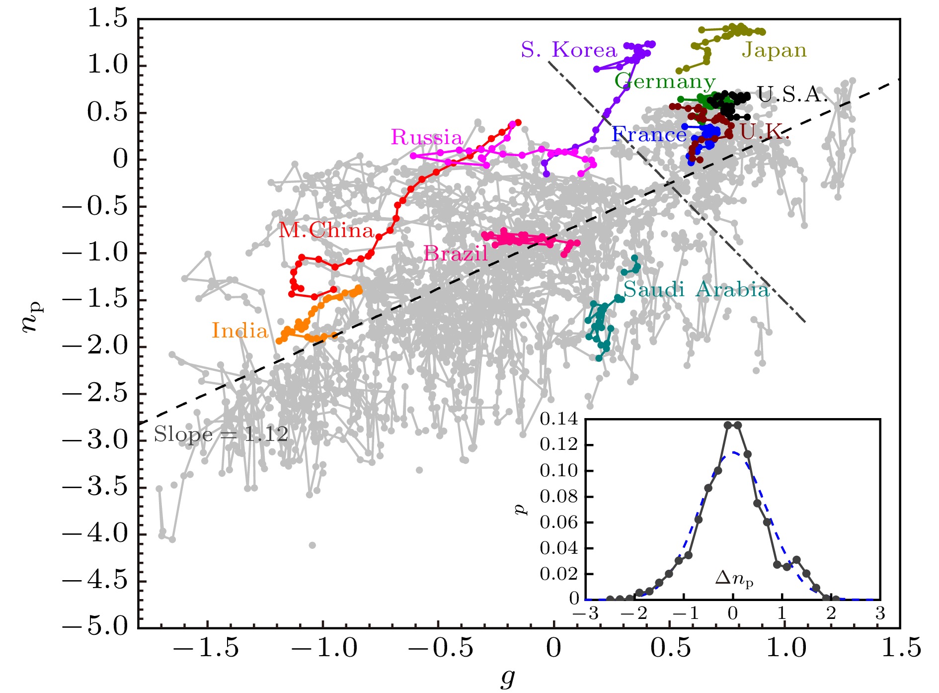 图 1 世界各经济体在由相对人均GDP的对数g和相对人均专利申请数的对数np(两者均以10为底数)所构成的空间中的变化轨迹. 彩色曲线为11个代表性经济体在该空间的轨迹, 灰色曲线为其他经济体. 灰色虚线为拟合直线np = 1.12g – 0.82. 灰色点划线大致区分了发达经济体的轨迹所在区域和发展中经济体所在区域, 右上方主要为发达经济体, 左下方主要为发展中经济体. 插图显示了各个数据点相对拟合直线的离差Δnp的概率分布, 蓝色虚线为其高斯函数拟合


 图 2 各经济体的区域创新指数I随年份的变化, 彩色线为11个代表性经济体, 灰色线为其他经济体
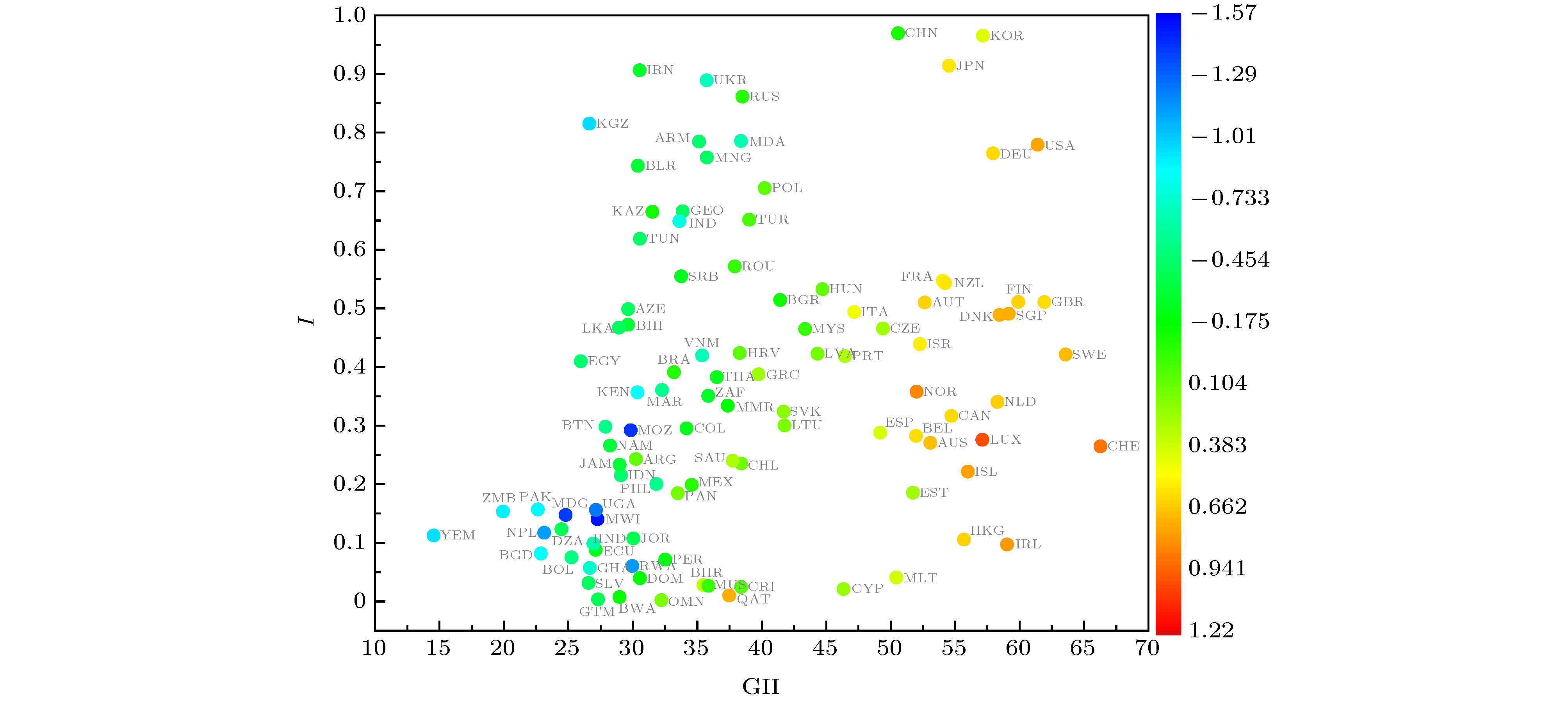 图 3 各经济体在2016年的区域创新指数I与该年份的全球创新指数(GII)的关系. 数据点的颜色表示该年份各经济体的相对人均GDP的对数值g


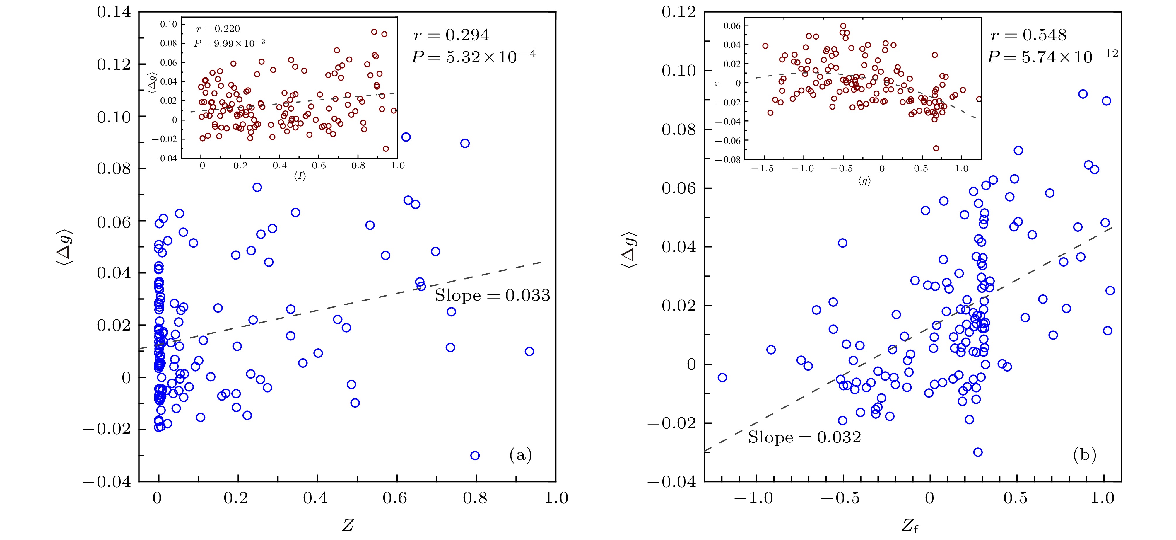 图 4 20年时间段(1998年至2017年)内各经济体平均区域创新指数


 图 5 以1年期、3年期和5年期为滑动窗口长度, 各类指标在滑动窗口期内各经济体的均值同相对人均GDP增长率的平均值


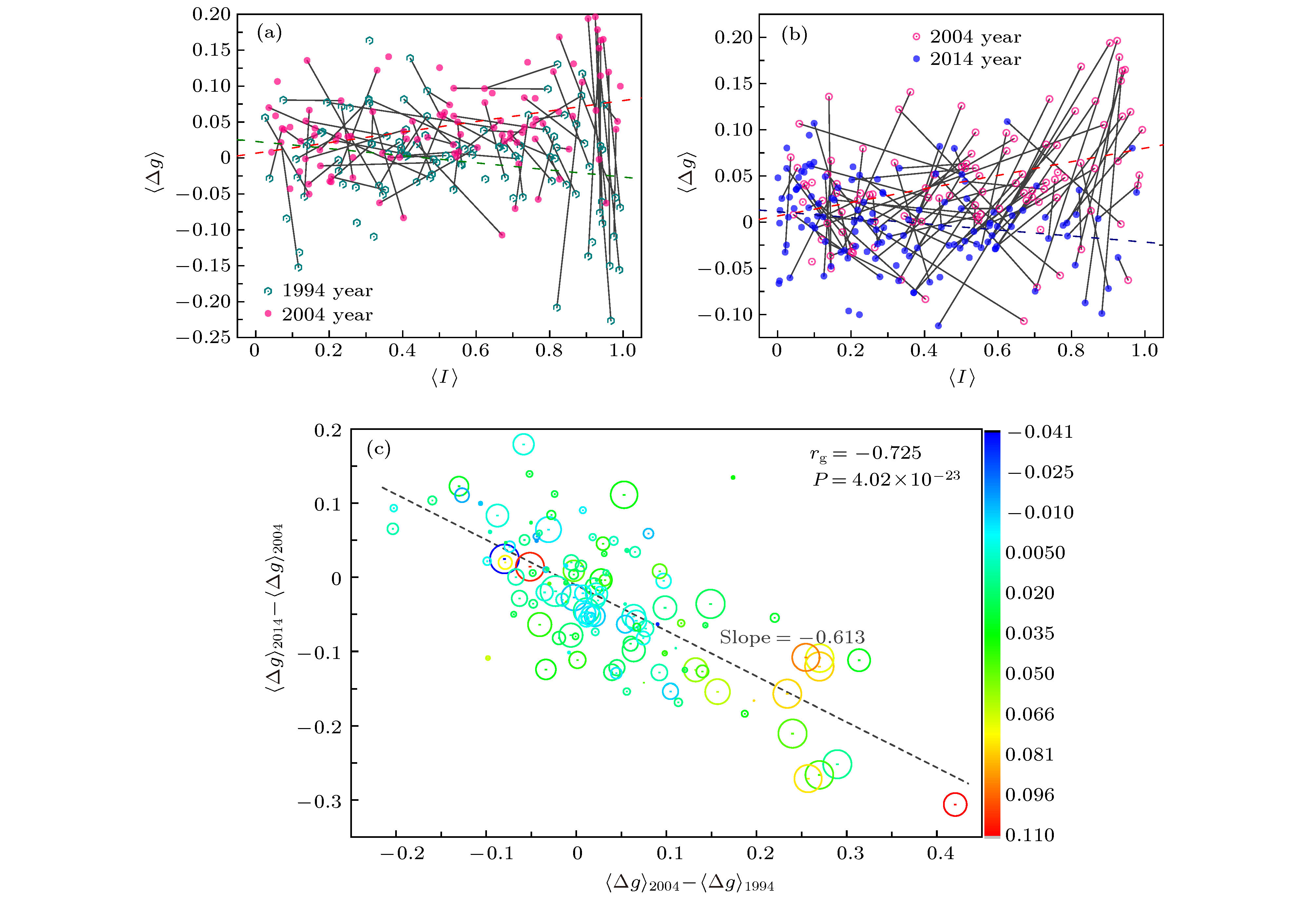 图 6 (a)和(b)分别对比了在谷-峰变换和峰-谷变换前后的两个典型年份的5年滑动窗口内各经济体的创新指数


