1.Key Laboratory of Underwater Acoustics Environment, Institute of Acoustics, Chinese Academy of Science, Beijing 100190, China 2.University of Chinese Academy of Science, Beijing 100049, China
Fund Project:Project supported by the National Natural Science Foundation of China (Grant No. 11874384)
Received Date:28 May 2019
Accepted Date:13 August 2019
Available Online:01 November 2019
Published Online:05 November 2019
Abstract:The field of ocean ambient noise contains numerous information about the water column, especially the information about the sub-bottom. The geoacoustics parameters of sub-bottom are very important factors influencing the spatial characteristics of ocean ambient noise field. For different layered structures of the sub-bottom, the bottom-loss shows different critical angles according to sound speed of each layer, while the structure of interference fringe is dependent on the thickness of the sediment. Flux theory of ocean ambient noise proposed by Harrison is used in this paper. Using this theory, the curve of bottom-loss can be extracted by computing the ratio between the energy of the upward wave and the downward wave. From the ideal reflection coefficient, the influence of sound speed, density and attenuation coefficient on reflection coefficient are discussed in the situation of the sub-bottom of acoustic half space, while the reflection coefficient of 1 layer of sediment is simplified. Initially, the reflection coefficient is the sum of sound waves reflect from the sub-bottom transmitted from the same source at the same angle. Only the first two terms are reserved, so that the mechanism of the interference fringe can be easily discussed. The structure of interference fringe can be explained which is affected by the thickness of the sediment. The curve of bottom-loss oscillates periodically with the increase of the thickness of the sub-bottom. Also by the reciprocity principle, the interference fringe of the reflection coefficient can be explained by considering the sound transmitted from two point sources at the surface of the sea. In this way the same result can be obtained as that from the method of simplification. The result of the experiment in China Yellow Sea shows that the information about the reflection coefficient of the sub-bottom can be extracted by the vertical azimuth spectrum of ocean ambient noise. In this way, the critical angle can be obtained, so that the sound speed of the sub-bottom can be estimated by using Snell law. The structure of the interference fringe is also contained in the bottom-loss curve estimated by ocean ambient noise. Therefore the layered structure, sound speed and the thickness of the layer of the sub-bottom can be estimated. Keywords:spatial characteristics of ocean ambient noise/ bottom-loss/ estimating geoacoustics parameters of sub-bottom
表1海水及海底声学参数 Table1.Parameters of ocean and sub-bottom
互谱密度矩阵直接利用OASES软件中的OASN模块计算获得[20], w设置为常规波束形成加权向量. 图2(a)为根据理想情况下真实反射系数公式求得的BL[21], 后文将对该公式进行讨论; 图2(b)是根据噪声垂直空间指向性利用OASN模块仿真得到的$\widehat {BL}$; 图2(c)提取出了1800 Hz下两种方法的掠射角BL曲线. 图2(a)和图2(b)中的条纹与图2(c)中的曲线峰值成对应关系, 阵元遍布全海深的理想状态下, 图2(c)中两条曲线的峰值一一对应, 仅在幅度上存在一定偏差, 因此利用Harrison能流理论估计海底反射损失是可行的. 图 2 (a) 真实反射损失BL; (b) 根据噪声垂直空间指向性利用OASN模块仿真得到的$\widehat {BL}$; (c) 1800 Hz下两种方法的比较, 实线为BL, 虚线为$\widehat {BL}$ Figure2. (a) True BL; (b) $\widehat {BL}$ computed by vertical directionality of ocean ambient noise using OASN; (c) two methods compare under 1800 Hz, the full line is BL, the imaginary line is $\widehat {BL}$
而在实际海上试验中, 阵元个数是有限的, 很难达到上述遍布全海深的理想状态. 有限的阵元个数会带来不同掠射角方向分辨率的下降, 这样会导致图2(b)中条纹信息一定程度上的缺失, 同时也使图2(c)中峰值的模糊, 但仍然有很多特征可以利用. 图3给出了两种不同海底分层结构的$\widehat {BL}$, 保留表1中的参数, 图中实线为间隔0.2 m的水听器遍布全海深的结果, 虚线为间隔0.2 m的42元水听器阵, 第一个阵元设置在水深30 m处, 频率均为1800 Hz. 海底模型如图4所示, 其中图4(a)为无限大液态声学半空间海底, 图4(b)为带有一层沉积层的海底. 图 3 1800 Hz下不同海底分层结构下的$\widehat {BL}$(实线为阵元遍布全海深, 点划线为42阵元, 间隔均为0.2 m) (a) 海底为无限大液体声学半空间; (b) 海底为单层沉积层 Figure3. The $\widehat {BL}$ of different structure of sub-bottom under 1800 Hz: (a) Infinite acoustic half space; (b) 1 layer of sediment. The full line corresponds to the condition that the elements set across the sea. The imaginary line corresponds to the condition that 42 elements set at the depth of 30 m
图 4 海底分层模型 (a)液体无限大声学半空间海底; (b) 存在一层沉积层海底 Figure4. Model of sub-bottom stratification: (a) Infinite acoustic half space; (b) 1 layer of sediment
图 13 第9组数据处理结果 (a) $\widehat {BL}$; (b) 1600 Hz下的$\widehat {BL}$曲线 Figure13. Results of the 9th set of data: (a) $\widehat {BL}$; (b) curve of $\widehat {BL}$ under 1600 Hz
图 14 第11组数据处理结果 (a) $\widehat {BL}$; (b) 1600 Hz下$\widehat {BL}$曲线 Figure14. Results of the 11th set of data: (a) $\widehat {BL}$; (b) curve of $\widehat {BL}$ under 1600 Hz
图 15 数据计算结果统计分布直方图 (a)沉积层声速; (b)基底声速; (c)沉积层厚度 Figure15. Statistical distribution histogram of 20 sets of data: (a) Sound speed of the sediment; (b) sound speed of the basement; (c) thickness of the sediment
为验证所估计沉积层厚度的可靠性, 试验船搭载了浅地层剖面仪(sub-bottom profiler), 该地层剖面仪发射调频信号, 利用声波在水中和水下沉积层内传播和反射的特性来探测海底地层结构. 图16给出了从试验点向东北方向扫描的海底地形, 35 m深处为海底表层, 在其下方存在沉积层, 图16(b)中用黑色标出, 厚度约为2.2 m, 噪声估计出的沉积层厚度与此结果基本符合. 图 16 浅地层剖面仪探测试验海区海底结构(图(b)中用黑点标明海底分界面) Figure16. Sub-bottom structure of the experimental area detected by sub-bottom profiler. The interface is marked by black spot in panel (b)
 图 1 浅海中利用垂直阵接收噪声空间结构


 图 2 (a) 真实反射损失BL; (b) 根据噪声垂直空间指向性利用OASN模块仿真得到的


 图 3 1800 Hz下不同海底分层结构下的

 图 4 海底分层模型 (a)液体无限大声学半空间海底; (b) 存在一层沉积层海底


 图 5 Pekeris分支割线、极点和积分的复波数平面


 图 6 不同谱域内噪声场的指向性和


 图 7 不同海底参数下的BL (a)衰减系数


 图 8 单层沉积层海底反射模型

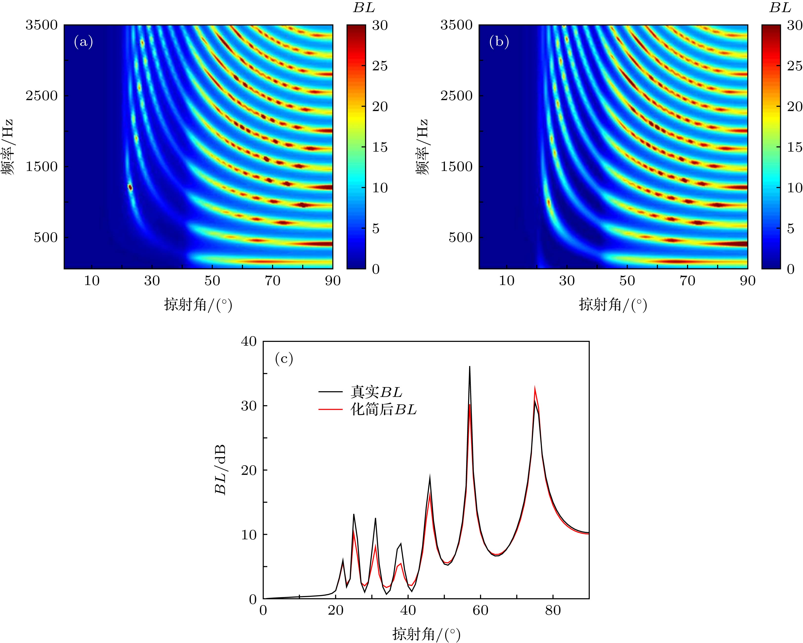 图 9 (a) (8)式计算的真实BL; (b) (10)式计算化简后的BL; (c) 1800 Hz下两条BL曲线


 图 10 (10)式计算化简后的BL (横轴利用(7)式转为


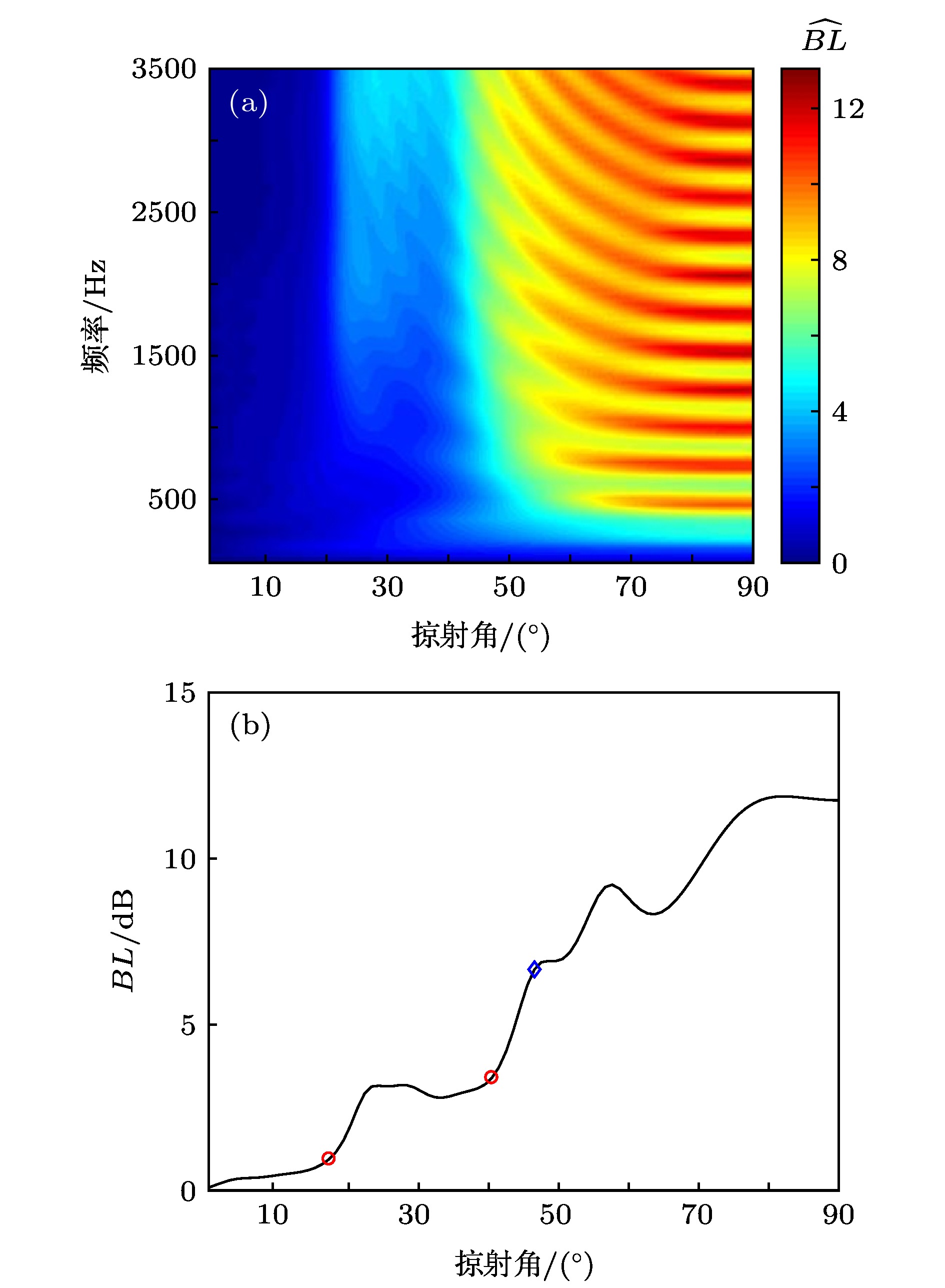 图 11 (a) 42阵元设置在水下30 m处


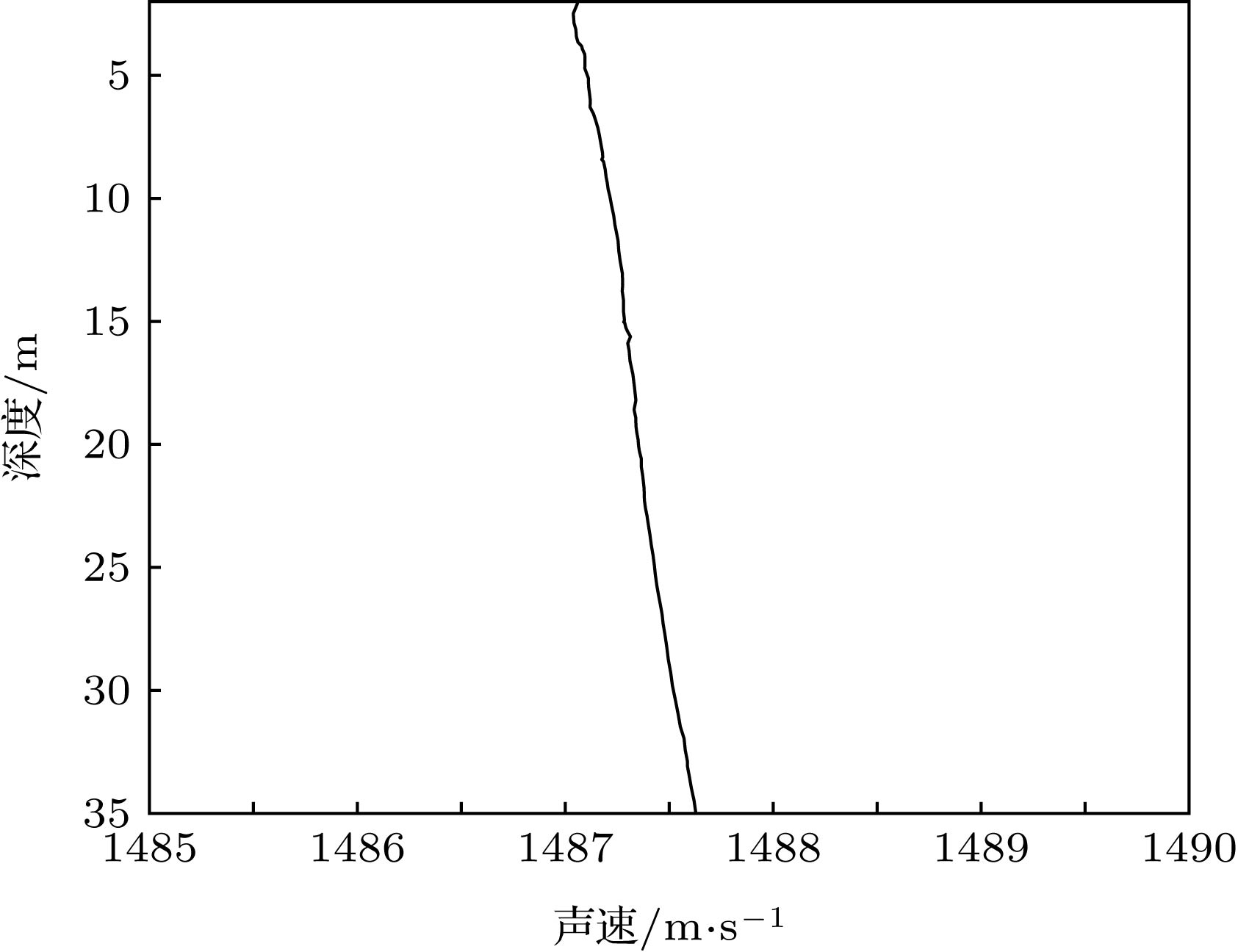 图 12 实验实测海水声速剖面
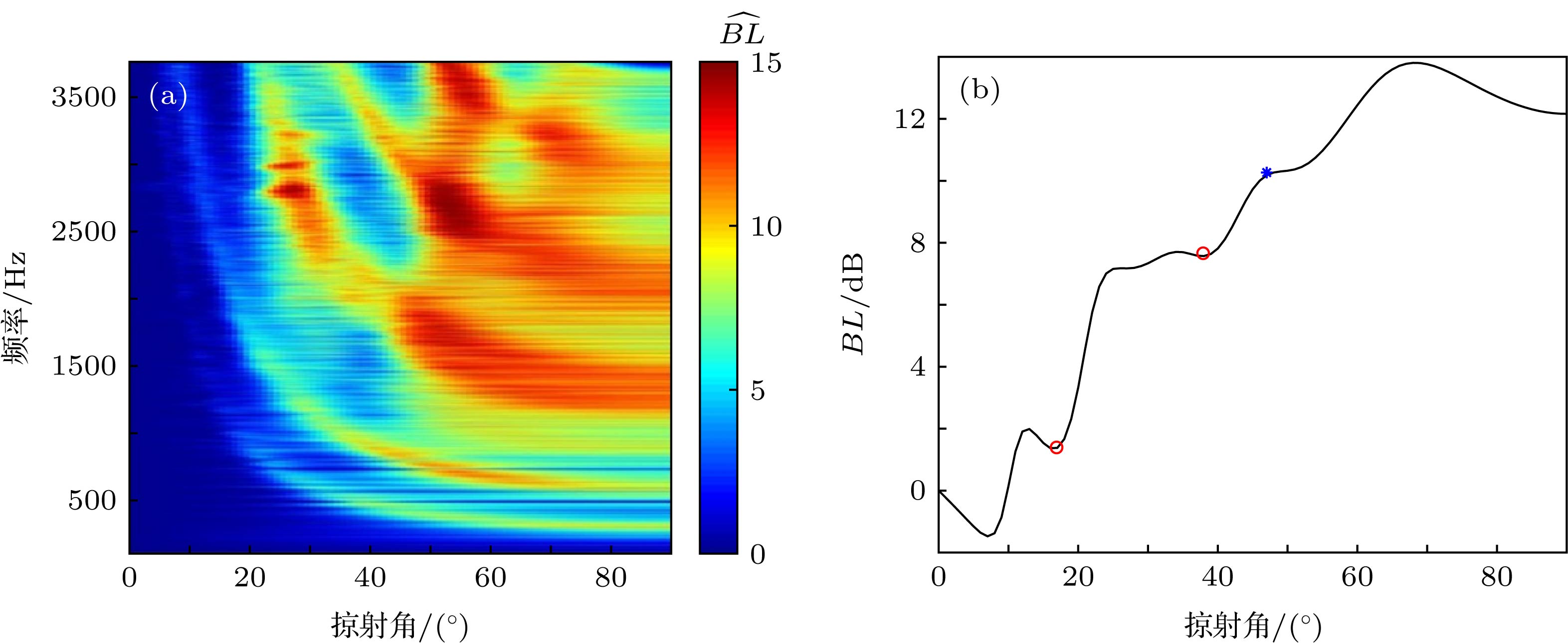 图 13 第9组数据处理结果 (a)


 图 14 第11组数据处理结果 (a)


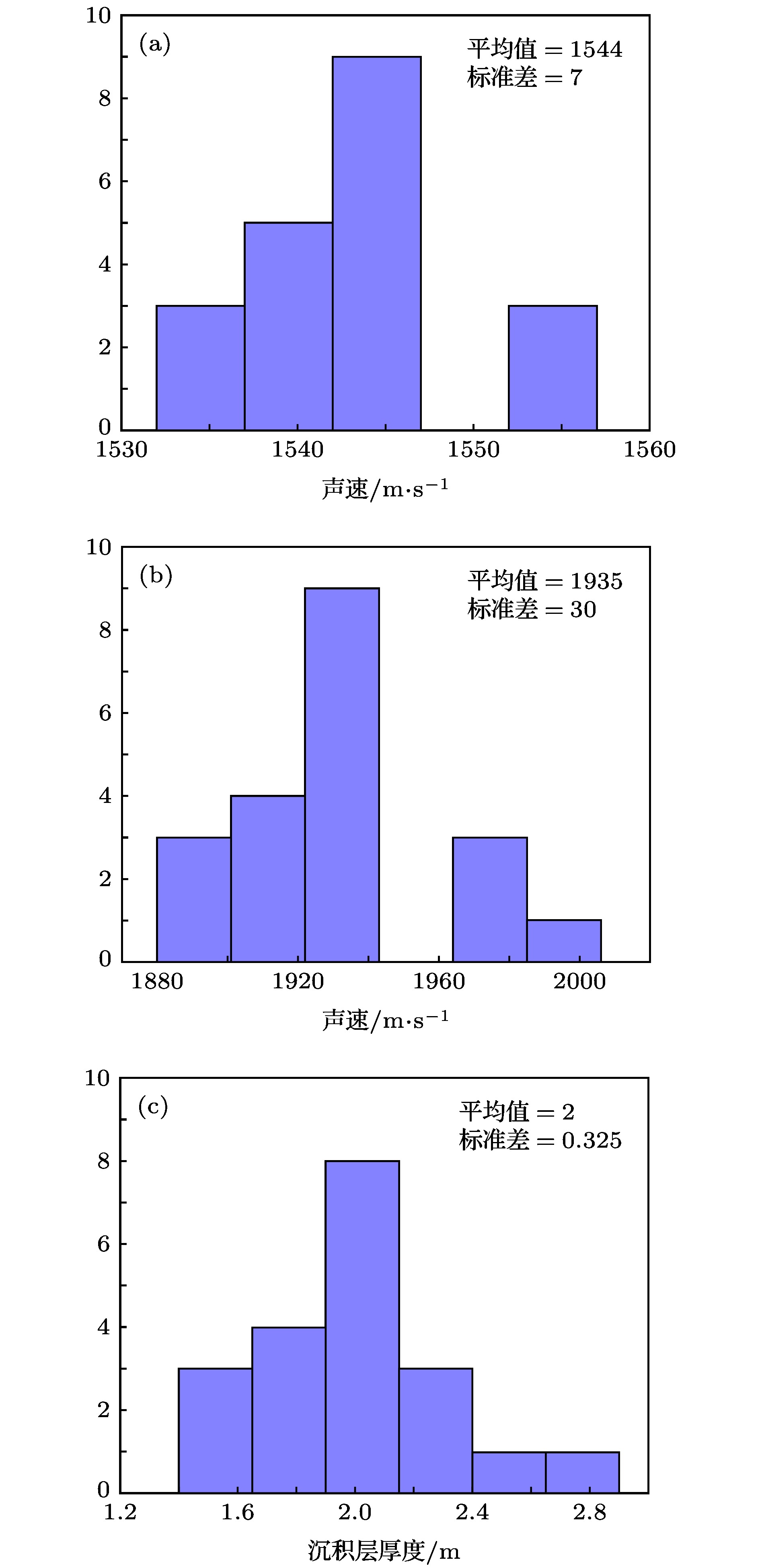 图 15 数据计算结果统计分布直方图 (a)沉积层声速; (b)基底声速; (c)沉积层厚度
 图 16 浅地层剖面仪探测试验海区海底结构(图(b)中用黑点标明海底分界面)


