刘卫东^1,2, 唐志鹏^,1,2, 夏炎³, 韩梦瑶¹, 姜宛贝¹1. 中国科学院地理科学与资源研究所 中国科学院区域可持续发展分析与模拟重点实验室,北京 100101
2. 中国科学院大学资源与环境学院,北京 100049
3. 中国科学院科技战略咨询研究院,北京 100190

Identifying the key factors influencing Chinese carbon intensity using machine learning, the random forest algorithm, and evolutionary analysis

LIU Weidong^1,2, TANG Zhipeng^,1,2, XIA Yan³, HAN Mengyao¹, JIANG Wanbei¹1. Key Laboratory of Regional Sustainable Development Modeling, Institute of Geographic Sciences and Natural Resources Research, CAS, Beijing 100101, China
2. College of Resources and Environment, University of Chinese Academy of Sciences, Beijing 100049, China
3. Institute of Science and Development, CAS, Beijing 100190, China

通讯作者: 唐志鹏(1978-), 男, 四川成都人, 博士, 副研究员, 研究方向为区域经济与区域可持续发展。E-mail:tangzp@igsnrr.ac.cn

收稿日期:2018-05-8修回日期:2019-10-17网络出版日期:2019-12-25

基金资助:

国家重点基础研究发展计划.2016YFA0602804 国家自然科学基金项目.41771135

Received:2018-05-8Revised:2019-10-17Online:2019-12-25

Fund supported:

The National Key Research and Development Program of China.2016YFA0602804 National Natural Science Foundation of China.41771135

作者简介 About authors
刘卫东(1967-),男,河北隆化人,研究员,中国地理学会会员(S110001202M),主要从事经济地理和区域发展研究E-mail:liuwd@igsnrr.ac.cn。







摘要
碳强度影响因子数量众多,通过在众多因子中评估其重要性以识别出关键影响因子进而解析碳强度关键因子的变化规律,是中国2030年碳强度能否实现比2005年下降60%~65%目标的科学基础。传统的回归分析方法对于评估众多因子的重要性存在多重共线性等问题,而机器学习处理海量数据则具有较好的稳健性等优点。本文从能源结构、产业结构、技术进步和居民消费等方面选取了56个中国碳强度影响因子指标,采用随机森林算法基于信息熵评估了1980-2014年逐年各项因子的重要性,通过指标数量与信息熵的对应关系统一筛选出每年重要性最大的前22个指标作为相应年度关键影响因子,最终依据关键影响因子的变化趋势划分了3个阶段作了演进分析。结果发现：1980-1991年,碳强度的关键因子主要以高耗能产业规模及占比、化石能源占比和技术进步为主;1992-2007年,中国经济进入快车道增长时期,服务业占比和化石能源价格对碳强度的影响作用开始显现,居民传统消费的影响作用在增大;2008年全球金融危机后,中国进入经济结构深化调整时期,节能减排力度大大增强,新能源占比和居民新兴消费的影响作用迅速显现。为实现2030年碳强度下降60%~65%目标,优化能源结构和产业结构,促进技术进步,提倡绿色消费,强化政策调控是未来需要采取的主要措施。
关键词： 机器学习;随机森林;碳强度;关键影响因子;中国

Abstract
As the Chinese government ratified the Paris Climate Agreement in 2016, the goal of reducing carbon dioxide emissions per unit of gross domestic product (carbon intensity) from 60% to 65% of 2005 levels must now be achieved by 2030. However, as numerous factors influence Chinese carbon intensity, it is key to assess their relative importance in order to determine which are most important. As traditional methods are inadequate for identifying key factors from a range acting simultaneously, machine learning is applied in this research. The random forest (RF) algorithm based on decision tree theory was proposed by Breiman (2001); this algorithm is one of the most appropriate because it is insensitive to multicollinearity, robust to missing and unbalanced data, and provides reasonable predictive results. We therefore identified the key factors influencing Chinese carbon intensity using the RF algorithm and analyzed their evolution between 1980 and 2014. The results of this analysis reveal that dominant factors include the scale and proportion of energy-intensive industries as well as fossil energy proportion and technical progress between 1980 and 1991. As the Chinese economy developed rapidly between 1992 and 2007, effects on carbon intensity were enhanced by service industry proportion and the fossil fuel price such that the influence of traditional residential consumption also increased. The Chinese economy then entered a period of deep structural adjustment subsequent to the 2008 global financial crisis; energy-saving emission reductions were greatly enhanced over this period and effects on carbon intensity were also rapidly boosted by the increasing availability of new energy and its residential consumption. Optimization of energy and industrial structures, promotion of technical progress, green consumption, and the reduction and management of emissions will be key to cutting future carbon intensity levels within China. These approaches will all help to achieve the 2030 goal of reducing carbon emission intensity from 60% to 65% of 2005 levels.
Keywords：machine learning;random forest;carbon intensity;key factor;China


PDF (1550KB)元数据多维度评价相关文章导出EndNote|Ris|Bibtex收藏本文
本文引用格式
刘卫东, 唐志鹏, 夏炎, 韩梦瑶, 姜宛贝. 中国碳强度关键影响因子的机器学习识别及其演进. 地理学报[J], 2019, 74(12): 2592-2603 doi:10.11821/dlxb201912012
LIU Weidong. Identifying the key factors influencing Chinese carbon intensity using machine learning, the random forest algorithm, and evolutionary analysis. Acta Geographica Sinice[J], 2019, 74(12): 2592-2603 doi:10.11821/dlxb201912012

1 引言

2016年,中国政府正式签署《巴黎协定》,标志着中国郑重承诺在2030年左右CO₂排放达到峰值,实现单位国内生产总值CO₂排放比2005年下降60%~65%的目标。如何实现这样的目标,不仅是中国政府面临的重大决策问题,也是全社会乃至国际社会关注的热点话题。张友国^[1]针对碳强度目标,研究了经济发展方式变化对中国碳强度的影响,认为改进能源结构有利于降低碳强度,居民消费增长不利于降低碳强度。Stern等^[2]认为中国要实现碳强度目标需要采取更强化的政策。Yuan等^[3]提出中国需要经济结构调整促进能源利用的显著减少。一个国家或地区碳排放总量取决于经济总量和碳强度（单位GDP的二氧化碳排放量）。由于中国仍是发展中国家,在相当长时期里追求适度的经济增长速度是实现国家富强的必要条件,故而不能寄希望通过降低经济增速来实现2030年碳峰值目标,而应着眼于碳强度的下降速度。

国内外****对于影响碳强度变化的因子解析主要从能源结构、产业结构、技术进步和居民消费以及土地利用等方面展开论述,他们认为优化能源结构有助于直接降低能源强度,进而降低碳强度^[4,5,6,7],通过调整产业结构促使低碳产业的占比上升也有助于降低碳强度^[8,9,10],采用先进的技术提升能源利用效率,有助于降低碳强度^[11,12,13],居民消费水平对于碳排放具有较强的增长作用^[14,15,16],不同的土地集约利用类型与碳排放效率之间并不保持普遍一致,存在一定的区域差异^[17,18,19]。这些因素主要由具体因子指标来体现,并且相互作用共同支配着碳强度的变化,这就需要建立较为全面的碳强度影响因子指标体系,以便更加细化的反映碳强度。通常在构建指标体系时,应遵循整体性原则、层次性原则和相关性原则,其中相关性原则要求设置的因子指标间既要相互联系、又要有所区别,避免重复、交叉指标使用造成信息重叠^[20]。毫无疑问地,这些具体因子作为社会生产力发展下的事物,对碳强度的影响并非恒定不变,在不同发展阶段,对于碳强度的重要程度也会不尽相同。因此,深入分析碳强度关键影响因子的历史变化趋势,通过寻求这些因子的演进规律是对中国碳排放未来长期趋势作出科学判断的决策基础,也是实现中国2030年碳排放峰值目标优化路径的根本保障。

目前对碳强度影响因子的解析方法主要集中在通径分析^[4]、面板数据模型^[5]、空间计量模型^[9]、自适应权重迪氏指数法^[21]、Laspeyres指数分解模型^[22]和Kaya恒等式分解^[23]等。通径分析、面板数据模型和空间计量模型均可认为是参数统计分析,而自适应权重迪氏指数法、Laspeyres指数分解模型和Kaya恒等式分解可归纳是因素分解分析,参数统计分析通常需要满足一定的统计前提假设,譬如需要因子间非强共线性保证参数估计方差最小从而使估计量有效,因素分解分析为满足恒等关系容易造成分解出的因子含义弱化,甚至解释较为片面。这些传统方法由于受限于经典的统计假设,选取碳强度影响因子的指标数目往往较少,能够识别出碳强度的关键影响因子数目就更少。对于政策指导而言,较少的影响因子意味着执行手段难以全面覆盖到经济社会各个方面,而以满足恒等关系人为分解的因子含义弱化,同样无法给出具体的指导意见。全球气候变化作为一个自然与社会交叉的综合问题,所涉及的影响因子也是数量众多,但是指标数量的增多容易造成分析的维数灾难,而机器学习通过大量数据的信息挖掘,在克服维数灾难上具有先天的优势。机器学习属于采用计算机模拟人类的学习算法,对已有数据进行学习策略的探索和潜在结构的发现,依据所得模型进行预测及分析^[24]。机器学习包括需要训练数据集的有监督学习和不需要训练数据集的无监督学习。传统解析因子的方法需要依靠样本数据按照设定固定算法流程进行计算获得参数结果,方法本身并不涉及不断自我学习进行改进运算结果的问题,而机器学习不仅参与样本数据运算挖掘信息,还通过机器不断自我学习,适应最优策略改变,不断得到新的改进结果,可以说机器学习过程本身就是一个不断改进运算结果的过程。此外,在有监督的学习中,机器学习可以结合多个弱监督模型得到一个更全面更优的强监督模型实现集成学习,能够有效提高决策结果的可靠性,目前集成学习仍然是机器学习中最热门的研究领域之一,现有的集成学习包括Bagging算法、Boosting算法和随机森林算法等^[25]。其中,随机森林算法具有分类精度高、运算速度快、运行结果稳健和泛化能力强的优点,在分类算法中得到了广泛应用。

鉴于此,本文采用随机森林算法从诸多碳强度影响因子中识别出关键影响因子,通过分析这些关键影响因子的历史演进规律,以期为相关部门提供中国2030年碳强度下降60%~65%目标的决策依据。

2 数据来源与研究方法

2.1 数据来源

1961-2014年的碳强度及其影响因子数据分别来自Maddison项目数据库、国际能源署（International Energy Agency, IEA）数据库、《中国能源统计年鉴》《中国工业统计年鉴》和《中国统计年鉴》。遵循已有的文献成果和因子指标间尽可能避免信息重叠^[20]的原则,从与碳强度密切相关的能源结构、产业结构、技术进步和居民消费方面选定了56个因子指标,并归纳为化石能源占比、化石能源价格、新能源占比、高能耗产业规模及占比、服务业占比、技术进步、居民传统消费和居民新兴消费9大类别（表1）。在中国碳强度及其因子数据选取方面,以中国统计年鉴资料为准,国外的数据资料作为参考,同时对部分缺失的资料进行了插值处理。

Tab. 1
表1
表1中国碳强度影响因子的类别和指标
Tab. 1Types and indexes of factors influencing Chinese carbon intensity

类别	具体因子指标(单位)	类别	具体因子指标(单位)
化石能源占比	煤炭占比(%)	高能耗产业规模及占比	纯碱(万t)
	石油占比(%)		烧碱(万t)
	天然气占比(%)		乙烯(万t)
化石能源价格	煤炭行业出厂价格指数		合成氨(万t)
	石油和天然气行业出厂价格指数		水泥(万t)
非化石能源占比	水电占比(%)		平板玻璃(万重量箱)
	沼气占比(%)		粗钢(万t)
新能源 占比	风电占比(%)		成品钢(万t)
	核能占比(%)		建筑业占比(%)
	光伏占比(%)		交通运输、仓储和邮政业占比(%)
	光热占比(%)	技术进步	全员劳动生产率(万元/人)
	地热占比(%)		发电及电站供热加工转换效率(%)
	液体生物燃料占比(%)		炼焦加工转换效率(%)
服务业 占比	金融业占比(%)		炼油加工转换效率(%)
	信息传输、计算机服务和软件业占比(%)		发电标准煤耗(克/千瓦时)
	教育业占比(%)		供电标准煤耗(克/千瓦时)
	卫生和社会保障社会福利占比(%)		发电厂线路损失率(%)
	文化体育娱乐业占比(%)		粗钢行业单位综合耗能(吨标煤/t)
	科学研究、技术服务和地质勘查业占比(%)		水泥行业单位综合耗能(千克标煤/t)
居民传统消费	城镇每百户私人汽车(辆)		乙烯行业单位综合耗能(吨标煤/t)
	城镇每百户摩托车(辆)		合成氨行业单位综合耗能(吨标煤/t)
	农村每百户摩托车(辆)		科技拨款占财政总支出的占比(%)
	城镇每百户电冰箱(台)		公共建筑单位面积耗能(千克标煤/m2)
	农村每百户电冰箱(台)		城镇居住建筑单位面积耗能(千克标煤/m2)
	城镇每百户电视机(台)		农村居住建筑单位面积耗能(千克标煤/m2)
	农村每百户电视机(台)	居民新兴消费	互联网宽带接入用户(万户)
	城镇每百户洗衣机(台)		高铁营业里程(km)
	农村每百户洗衣机(台)		电子商务交易额(万亿)

新窗口打开|下载CSV

2.2 随机森林算法

随机森林算法是2001年Breiman基于决策树提出的一种集成学习方法。随机森林的“随机”体现在训练每棵树时,从全部训练样本中随机选取一个同样大小数据集进行训练,数据集中元素选取的方式为Bootstrap抽样技术。同时在树的每个分支节点变量,随机性选取所有特征的若干个子集通过纯度计算（如信息增益、信息增益率和基尼系数等）获得子集特征划分的最佳分割方式。“森林”则体现在让每颗树充分生长,并不剪枝,树的不同数量也影响着最终决策值。当树的增加对最终决策值并无显著变化,树的数量增多只会增加计算量,此时“森林”规模确定。随机森林对多重共线性不敏感,对缺失数据和非平衡的数据也比较稳健,能够提供合理的预测结果^[26],是当前采用机器学习处理高维属性数据最好的算法之一。目前随机森林算法主要基于Bootstrap抽样技术和CART算法两个模块来完成。

2.2.1 Bootstrap抽样技术 随机森林是利用Bootstrap抽样方法从原始样本中抽取多个样本,对每个Bootstrap样本进行决策树建模,然后将这些决策树组合起来,通过投票得分规则获得最终结果^[27]。Bootstrap抽样^[28]是从原始样本容量 N的训练集合 T中有放回地随机抽取 N个样本生成新的训练样本集,独立抽样 m次,生成 m个相互独立的Bootstrap样本集。Bootstrap抽样过程中每个样本未被抽取的概率P_i为：

（1）Pi=1-1NN,(i=1,2,?,N)
当 N值足够大时,每个样本未被抽取的概率为：

（2）limN→∞1-1NN=limU→-∞1+1UU-1=e-1≈0.37
表明原始样本集T中大约37%的样本不会出现在Bootstrap样本中,这些数据也称为袋外（Out of Bag, OOB）数据。随机森林算法正是利用Bootstrap抽样技术生成多个训练样本集,构建多个分类器,从而形成“森林”分类器。Bootstrap采用随机独立的有放回抽样,可以尽量避免随机未抽样带来的信息损失,克服了样本类别不平衡带来的负面影响,提高算法可靠性。

2.2.2 决策树CART算法 决策树作为一种树状模型,包括根节点、中间节点和叶子节点,每个节点表示对象的属性,从根节点经过中间节点最后到叶子节点的路径表示某种决策规则。决策树生成时,主要采用一种递归的方式,从根节点开始,分成两颗子树,从子树开始,又继续产生根节点和左右子树,每颗子树继续递归生成新的子树,直到产生叶子节点为止。决策树的生成算法很多,包括CLS、ID3、C4.5和CART等节点分裂算法^[29]。在CLS算法中,节点分裂过程是随机的,有多少属性的值域就对应多少分支,每个节点都按照该思路产生新的分支,直到产生叶子节点才终止算法,该方法导致选取不同的测试属性结果也存在差异。针对CLS算法没有规定采用何种测试属性带来算法不确定性,ID3算法在采用属性时都遵守一个固定规则,通过引入信息熵对属性的纯度划分进行计算比较,选择最大属性的信息增益作为测试属性。C4.5算法针对ID3算法中信息增益偏离的问题,引入分裂信息比率指标,计算信息增益率使得选取的属性比较均匀,避免产生偏向性。

CART（Classification and Regression Tree）算法由Breiman等于1984年提出^[30],同样以信息熵为理论基础,以递归构建决策树产生决策为规则思想,基于 Gini系数划分属性纯度, Gini系数越小,属性划分纯度越大,选取 Gini系数最小的划分构建决策树。CART算法是目前在随机森林中构建决策树比较普遍的一种算法,具体算法流程为^[29]：

① 连续特征变量的离散化。对于N个样本的连续特征A有N个,从小到大排列为 a1,a2,?,aN相邻两样本取中位数,一共取N-1个离散划分,第i个划分点S_i表示为：

（3）Si=ai+ai+12
② 计算每个划分的基尼系数 GiniP。假如有K个类别,第i个类别出现概率为P_i,基尼系数表达式为：

（4）GiniP=∑i=1KPi1-Pi=1-∑i=1KPi2
对于给定的样本T,假设K个类别,第 i个类别出现的数量为T_i,则样本T的基尼系数表达式为：

（5）GiniP=1-∑i=1KTiT2
当根据特征A的某个值a,把T划分为T₁和T₂两部分,则在特征A的条件下,T的基尼系数表达式为：

（6）GiniT,A=T1TGiniT1+T2TGiniT2
③ 对于当前节点的数据集,按照基尼系数最小原则进行节点分裂,通过递归形式一直完成决策树的构建。

2.2.3 随机森林算法流程 随机森林算法在上述Bootstrap抽样和CART算法基础上完成,具体流程^[29]如下：

① 产生训练集。每一棵树对应一个训练集,要构建N棵决策树,需要产生N个训练集。每个训练集通过Bootstrap抽样后产生子训练集,通过对所有子训练集进行综合集成预测结果,由于子训练集间会产生较大差异,增加了多样性,保证结果的稳健性。

② 构建每棵决策树。主要从根节点、中间节点到叶子节点通过节点分裂规则,包括信息增益最大、信息增益率最大和Gini系数最小等原则,通常采用CART算法里Gini系数最小进行节点分裂,不断重复该分裂,其中每次节点分裂让所有的属性按照某种概率分布随机选择其中某几个属性参与节点的分裂过程。每棵子树的生长过程中,不是将全部M个输入变量参与节点分裂,而是随机抽取F（F ≤ M）个随机特征变量,F的取值一般为 log2M+1。

③ 形成森林。重复上述两个步骤建立大量的决策树,就生成了随机森林。用森林中每棵树为OOB中的样本进行分类,统计每个类别获得的投票数,得票数最多的类别被认为是样本的类别,OOB中未被正确分类的样本比例为袋外分类错误率。

随着随机森林中一系列决策树 kx1,kx2,?,kxN中数量N的增加,对几乎所有的随机变量序列 θ1,θ2,?,θk,随机森林的泛化误差 GE*收敛如公式（7）所示^[27]。这表明泛化误差 GE*趋向一个概率上限,不会随着决策树增加产生过拟合的问题,具有较好的稳健性。

（7）limN→∞GE*=PxyPθkx,θ=Y-maxj≠YPθkx,θ=j<0
式中：y为正确分类向量;j为不正确分类向量;P_xy代表随机变量x和y的联合概率;P_θ代表随机变量θ的概率。

3 实证分析

3.1 中国碳强度关键影响因子的机器学习识别

鉴于机器学习的可靠性往往需要充足的样本数,首先基于每20年样本数作为一个数据集,并且逐年向后滑动依次获得1980-2014年每年的数据集,每个数据集均有上千个指标数目,保证了样本数的充足。其次,根据上述Bootstrap抽样技术对每个数据集建立生成训练集并进行训练,再基于CART算法对每个训练集做不同节点分裂的属性划分,节点分裂一直持续到公式（6）中Gini系数最小,这样保证了所有划分都是纯度最大的,每个纯度最大的划分就是一个决策树,通过不断重复前面抽样训练和节点划分,建立多棵决策树就完成了随机森林的生成,上述机器学习过程主要在计算机R软件中编程实现。

在已完成的节点分裂属性划分的数据集中,Gini系数大小反映了决策树属性划分的纯度,Gini系数越小,决策树节点划分的纯度越大,对森林中所有决策树的节点变量进行属性划分,计算平均Gini系数的减小程度,当减小程度很大时,表示森林中所有决策树平均纯度大幅提高,表明该节点变量对森林的影响很大。因此只要计算每个数据集中不同指标的 Gini系数减小值,根据Gini系数减小值可以评价出1980-2014年中国碳强度影响因子指标逐年的重要程度。由于随机森林中Gini系数是基于信息熵计算获得,根据熵值可加性,意味着所有影响因子的Gini系数减小值总和也就代表了整个碳强度因子指标体系的重要性。因此,为统一设定中国碳强度关键因子筛选的指标数量阈值,对1980-2014年每年各项指标的Gini系数减小值均由大到小排序,再计算各项指标在1980-2014年的平均值,得到碳强度因子指标数量与样本均值的Gini系数减小值对应关系（表2）。

Tab. 2
表2
表2碳强度因子指标数量与样本均值的Gini系数减小值
Tab. 2Carbon intensity indicator values and corresponding average Gini coefficient reductions

碳强度因子指标数量	1	2	3	4	5	6	7	8
Gini系数减小值	0.784	0.655	0.525	0.449	0.407	0.390	0.380	0.371
碳强度因子指标数量	9	10	11	12	13	14	15	16
Gini系数减小值	0.360	0.350	0.342	0.335	0.328	0.321	0.310	0.302
碳强度因子指标数量	17	18	19	20	21	22	23	24
Gini系数减小值	0.292	0.287	0.278	0.268	0.263	0.250	0.229	0.201
碳强度因子指标数量	25	26	27	28	29	30	31	32
Gini系数减小值	0.194	0.189	0.184	0.180	0.175	0.170	0.166	0.160
碳强度因子指标数量	33	34	35	36	37	38	39	40
Gini系数减小值	0.154	0.147	0.142	0.135	0.127	0.115	0.106	0.085
碳强度因子指标数量	41	42	43	44	45	46	47	48
Gini系数减小值	0.078	0.072	0.067	0.060	0.054	0.046	0.037	0.032
碳强度因子指标数量	49	50	51	52	53	54	55	56
Gini系数减小值	0.028	0.027	0.024	0.021	0.018	0.014	0.010	0.005

新窗口打开|下载CSV

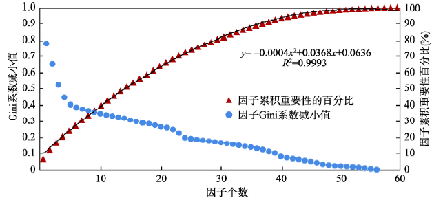
显然地,对中国碳强度重要程度高的影响因子属于关键因子。在中国碳强度关键因子的数量划分上,数量不宜过多,否则失去了识别关键因子的意义,但同时也不能数量过少,否则难以较全面的涵盖整个碳强度因子指标体系的重要性。鉴于此,本文根据大多数2/3的原则,即设定的指标数量阈值能涵盖整个碳强度因子指标体系重要性的2/3以上,即可作为关键因子。按照表2结果可以计算得到,随着从第1个因子增加到第56个因子,因子累积的重要性由6.7%增加到100.0%（图1）。

图1

新窗口打开|下载原图ZIP|生成PPT
图11980-2014年碳强度因子的Gini系数减小平均值和累积重要性百分比

Fig. 1Average Gini coefficient reductions during the period from 1980 to 2014 and the corresponding cumulative percentage importance of carbon intensity indicators



根据图1所示结果,前22个指标累积涵盖了整个碳强度因子指标体系70%左右的重要性,从指标数量来看,不到一半数量的指标涵盖了全部指标2/3以上的重要性。因此,本文设定识别关键因子的指标数量为22。各年度Gini系数减小值由大到小前22个指标可作为1980-2014年关键影响因子。譬如根据Gini系数减小值由大到小,1980年中国碳强度前5个关键影响因子指标依次是天然气占比、发电标准煤耗、合成氨、烧碱和乙烯行业单位综合耗能;1981年依次为天然气占比、供电标准煤耗、全员劳动生产率、水泥行业单位综合耗能和乙烯行业单位综合耗能;…;1991年依次为石油占比、煤炭占比、城镇每百户摩托车、天然气占比和合成氨;…;2000年依次为建筑业占比、城镇每百户私人汽车、粗钢行业单位综合能耗、发电厂线路损失率和乙烯行业单位综合能耗;…;2010年依次为煤炭占比、信息传输计算机服务和软件业占比、科技拨款占财政总支出占比、地热占比和农村每百户电视机;…;2014年依次为煤炭占比、水电占比、炼焦加工转换效率、城镇每百户洗衣机和公共建筑单位面积耗能。从1980-2014年逐年筛选出前22个中国碳强度关键影响因子,对这些具体因子指标按照表1归类并统计各类别的指标数量（表3）。

Tab. 3
表3
表31980-2014年中国碳强度关键影响因子的类别及指标数量
Tab. 3Key influencing factors and values for Chinese carbon intensity between 1980 and 2014

类别\年份	1980	1981	…	2000	…	2010	…	2013	2014
化石能源占比	3	3	…	0	…	1	…	2	1
化石能源价格	0	0	…	0	…	0	…	2	2
可再生能源(水电和沼气)占比	0	0	…	0	…	0	…	1	1
新能源占比	0	0	…	0	…	1	…	1	2
高耗能产业规模及占比	8	8	…	7	…	6	…	4	4
服务业占比	0	0	…	1	…	2	…	2	2
技术进步	8	8	…	6	…	4	…	3	5
居民传统消费	3	3	…	8	…	6	…	5	4
居民新兴消费	0	0	…	0	…	2	…	2	1
合计	22	22	…	22	…	22	…	22	22

注：限于篇幅,仅列出1980年、1981年、2000年、2010年、2013年和2014年的指标统计数。

新窗口打开|下载CSV

3.2 中国碳强度关键影响因子的历史演进分析

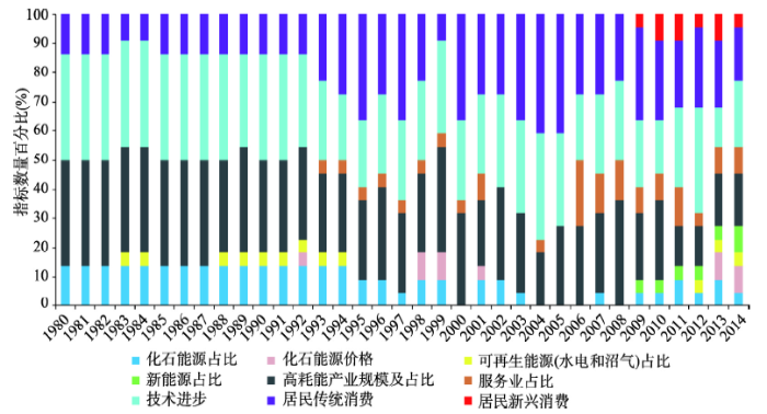
根据表3中1980-2014年中国碳强度关键影响因子的类别及其所含指标数量计算其百分比（图2）,某个类别因子所在年度中占的百分比越高,表明该类别因子对碳强度的影响程度越大。

图2

新窗口打开|下载原图ZIP|生成PPT
图21980-2014年中国碳强度关键影响因子的9类指标数量百分比图

Fig. 2Graphs to show percentages of nine key factors influencing Chinese carbon intensity between 1980 and 2014



根据图2显示结果,在1980-2014年期间,对中国碳强度关键影响因子大体呈现两种特征：① 因子对中国碳强度的影响较为稳定,并未随着时间变化呈现出明显的时间特征,如化石能源占比、高能耗产业、技术进步和居民传统消费对碳强度一直占据着比较重要的影响。此外从居民消费对碳强度影响来看,无论是家电消费因子还是家用交通工具消费因子农村居民与城镇居民并无显著差异,绿色消费适用于所有居民,也适用于一切家用耗能品。因此对于这些因子,减排调控需要保持一贯性,做到持之以恒。② 因子对中国碳强度的影响具有明显的时间特征,譬如在能源结构方面,可再生能源（主要是水电占比）早期对碳强度影响较大,进入2009年起,新能源占比（地热和光热）影响显现;在产业结构方面,早期服务业占比对碳强度的影响不明显,1993年开始金融业占比影响作用开始显现,2006年以后信息传输、计算机服务和软件业占比对碳强度一直起着显著的影响,科学研究、教育业、文化和娱乐产业占比对碳强度影响也开始显现;在居民新兴消费方面,2009年起互联网宽带接入用户数对碳强度的影响作用开始显现,2010年起电子商务交易额对碳强度的影响显著增大。因此对于这些因子,未来需要充分考虑到对碳强度影响随时间变化的特征,做到减排调控措施与时俱进。

总体来看,中国碳强度关键影响因子的历史演进可以大概分为3个阶段：① 20世纪80年代初期至1991年,中国碳强度的关键影响因子主要是高能耗产业规模及占比、化石能源占比、技术进步和居民传统消费。这一时期中国经济质量不高,发展方式较为粗放,经济结构以高耗能工业为主,能源消费结构也主要以煤炭为主,发电煤耗等生产性因素对中国碳强度一直起着决定性的影响作用,因此在早期中国经济发展阶段中,对于碳强度的降低措施主要需从生产因素考虑。② 1992-2007年,1992年邓小平开始南巡讲话,中国经济得到进一步深化改革开放,经济增速步入快车道,同期中国居民收入不断增加,居民家电和家用交通工具的消费也在快速增长。1993年中国首次由石油出口国转为石油净进口国,对于能源需求也在增大。2001年中国加入世界世贸组织（WTO）,对外开放进一步扩大,电子信息技术也得到了飞速发展,国民经济中服务业占比开始稳步上升。这一时期,关键影响因子除了高能耗产业规模及占比、化石能源占比和技术进步,居民传统消费影响作用明显加大,服务业占比和化石能源价格对于碳强度的关键影响也开始显现。因此,这个阶段对碳强度影响由早期的生产因素主导转变为生产与消费因素影响并重,对于碳强度的降低措施则需从生产和消费两方面因素考虑。③ 2008-2014年,2008年全球金融危机后,中国经济结构开始深化调整,开始加大节能减排的措施,新能源的使用也进一步得到了政府的大力支持,并且各种节能减排技术的科技研发投入也在不断增长。随着互联网技术的发展和中国高铁大规模投入运营,互联网已普遍性融入居民生活中,高铁出行大大缩短了通勤时间,电子商务规模也在不断增大。这一阶段新兴产业和新兴消费对碳强度影响显著增强,关键影响因子除了高能耗产业规模及占比、化石能源占比、技术进步、居民传统消费、服务业占比、化石能源价格外,新能源占比、居民新兴消费和科技拨款占财政总支出的占比对于碳强度的影响作用也开始显现。这说明除了居民传统消费外,居民新兴消费对碳强度的影响也很重要,是未来制定节能减排政策需要重视的一个方向。

4 结论及启示

全球气候变化是一个涉及自然与社会交叉的综合性问题,发展低碳经济是应对全球气候变化的唯一路径选择。中国作为负责任的大国承诺在2030年实现碳强度比2005年下降60%~65%的目标。要实现这样的目标,首先必须明确影响碳强度的关键因子,政策手段作用于关键因子才能实现降低碳强度的目标。鉴于传统定量方法的不足,本文采用了机器学习算法来识别中国碳强度的关键影响因子并作了历史演进分析,文中得到的结论及启示如下：

（1）通过随机森林算法识别出1980-2014年中国碳强度逐年的关键影响因子,发现不同的发展阶段,对碳强度起着影响作用的关键因子也在发生着变化,因此中国的节能减排政策也应适时调整,而非一成不变。1980年至1991年碳强度的关键因子主要以高耗能产业规模及占比、化石能源占比和技术进步为主;1992年邓小平南巡讲话至2007年,中国经济进入快车道增长时期,服务业占比和化石能源价格对碳强度的影响作用开始显现,居民传统消费的影响作用在增大;2008年全球金融危机后,中国进入经济结构深化调整时期,节能减排力度大大增强,新能源占比和居民新兴消费对碳强度的影响作用开始显现。总体来看,降低化石能源占比和高耗能产业规模及占比、推动技术进步是必须倡导的减排措施;大力发展服务业,优化产业结构,通过财税政策刺激化石能源市场价格来减少化石能源的使用,进而推动新能源发展也是需要实施的政策手段;提倡城乡绿色消费包括传统家电和家用交通工具消费以及近几年逐渐新兴起来的互联网电子商务等消费,则是现在乃至未来降低碳强度应该关注的重要方向。

（2）随着全球气候变化问题得到广泛重视,人们在追求经济增长的同时,也对环境可持续发展提出了要求。碳强度与社会生产和居民生活众多方面紧密相连,不同的经济发展阶段影响碳强度的关键因子有所差异,本文的研究分析也论证了这一观点。传统的参数统计分析由于需要克服多重共线性的影响无法解决碳强度的因子数量过多的问题,而因素分解分析为满足恒等关系分解出的因子含义弱化,甚至解释较为片面性。机器学习有处理海量数据的先天优势,其中随机森林算法具有良好的稳健性和泛化能力。但是地缘环境演变、新技术和新产业涌现带来未来社会经济发展的不确定性,随机森林算法识别碳强度关键因子的参数对不确定情景的适用性还需要作进一步深入分析。就总体而言,由于受到社会经济系统发展的惯性影响,中国碳强度未来影响因子的重要性毫无疑问仍然会与其历史演进的轨迹保持着密切相关。实现2030年中国碳强度目标需要制定清晰明确的战略思路,超前部署,并采取强有力的政策措施。因此,把握中国碳强度关键因子的历史演进规律对于未来我们将要采取的政策措施具有重要的参考价值。

参考文献 View Option 原文顺序
文献年度倒序
文中引用次数倒序
被引期刊影响因子

[1] Zhang Youguo . Economic development pattern change impact on China's carbon intensity
Economic Research Journal, 2010(4):120-133.
[本文引用: 1]

[ 张友国 . 经济发展方式变化对中国碳排放强度的影响
经济研究, 2010(4):120-133.]
[本文引用: 1]

[2] Stern D, Jotzo F . How ambitious are China and India's emissions intensity targets?
Energy Policy, 2010,38(11):6776-6783.
DOI:10.1016/j.enpol.2010.06.049URL [本文引用: 1]

[3] Yuan J, Hou Y, Xu M . China's 2020 carbon intensity target: Consistency, implementations, and policy implications
Renewable and Sustainable Energy Reviews, 2012,16(7):4970-4981.
DOI:10.1016/j.rser.2012.03.065URL [本文引用: 1]

[4] Wang Shaohua, Yu Weiyang . Sensitivity analysis of primary energy consumption structural change and carbon intensity
Resources Science, 2013,35(7):1438-1446.
[本文引用: 2]

[ 王韶华, 于维洋 . 一次能源消费结构变动对碳强度影响的灵敏度分析
资源科学, 2013,35(7):1438-1446.]
[本文引用: 2]

[5] Peng Xu, Cui Herui . Research on the effects of energy structure adjustment in china on carbon intensity
Journal of Dalian University of Technology (Social Sciences), 2016,37(1):11-16.
[本文引用: 2]

[ 彭旭, 崔和瑞 . 中国能源结构调整对碳强度的影响研究
大连理工大学学报(社会科学版), 2016,37(1):11-16.]
[本文引用: 2]

[6] Li H, Wang L, Shen L , et al. Study of the potential of low carbon energy development and its contribution to realize the reduction target of carbon intensity in China
Energy Policy, 2012,41:393-401.
DOI:10.1016/j.enpol.2011.10.061URL [本文引用: 1]
Appraising low carbon energy potential in China and studying its contribution to China's target of cutting CO2 emissions by 40-45% per unit of GDP by 2020 is crucial for taking countermeasures against climate change and identifying low carbon energy development strategies. This paper presents two scenarios and evaluates the development potential for low carbon energy and its various sources. Based on the evaluation, we analyze how low carbon energy contributes to achieving China's national target of carbon intensity reduction. We draw several conclusions from the analysis. First, low carbon energy will contribute 9.74% (minimum) to 24.42% (maximum) toward the 2020 carbon intensity target under three economic development schemes. Second, the contribution will decrease when the GDP growth rate increases. Third, to maintain the same contribution with high GDP growth rates, China should not only strengthen its investment and policy stimulation for low carbon energy but also simultaneously optimize economic structures and improve carbon productivity. (C) 2011 Elsevier Ltd.

[7] Fan Y, Liu L C, Wu G , et al. Changes in carbon intensity in China: Empirical Findings from 1980-2003
Ecological Economics. 2007,62(3/4):683-691.
DOI:10.1016/j.ecolecon.2006.08.016URL [本文引用: 1]

[8] Zhang Y G . Structural decomposition analysis of sources of decarbonizing economic development in China: 1992-2006
Ecological Economics, 2009,68(8/9):2399-2405.
DOI:10.1016/j.ecolecon.2009.03.014URL [本文引用: 1]

[9] Feng Yan, Zhu Lingyun, Zhang Dahong . Spatial and econometric analysis of effect of industrial structure adjustment on carbon intensity in China
Soft Science, 2017,31(7):11-15.
[本文引用: 2]

[ 冯彦, 祝凌云, 张大红 . 中国产业结构调整对碳强度影响的空间计量研究
软科学, 2017,31(7):11-15.]
[本文引用: 2]

[10] Xu Hui, Wang Hui . The impact of industrial structure adjustment on China's carbon intensity goal: The outlook of 2020
Science and Technology Management Research, 2016,36(13):232-236.
[本文引用: 1]

[ 徐辉, 王慧 . 产业结构调整对中国碳强度目标实现的影响: 展望2020年
科技管理研究, 2016,36(13):232-236.]
[本文引用: 1]

[11] Yan Zheming, Deng Xiaolan, Yang Zhiming . The impact of heterogeneous technological innovation on carbon intensity: A global evidence based on patent statistics
Journal of Beijing Institute of Technology (Social Sciences Edition), 2017,19(1):20-27.
[本文引用: 1]

[ 鄢哲明, 邓晓兰, 杨志明 . 异质性技术创新对碳强度的影响: 基于全球专利数据
北京理工大学学报(社会科学版), 2017,19(1):20-27.]
[本文引用: 1]

[12] Huang Jie, Ding gang . A research on the threshold effect of the impact of technical progress on carbon intensity
Science & Technology Progress and Policy, 2014,31(18):22-26.
DOI:10.1111/cxo.13030URLPMID:31852027 [本文引用: 1]
In ageing populations, the prevalence of chronic diseases such as glaucoma is projected to increase, placing additional demands on limited health-care resources. In the UK, the demand for secondary care in hospital eye clinics was inflated by high rates of false positive glaucoma referrals. Collaborative care models incorporating referral refinement, whereby glaucoma suspect referrals are triaged by suitably trained optometrists through further testing, can potentially reduce false positive referrals. This study examined the impact of a referral refinement model on the accuracy of glaucoma referrals in Australia.
[ 黄杰, 丁刚 . 技术进步对碳强度影响的门槛效应研究
科技进步与对策, 2014,31(18):22-26.]
DOI:10.1111/cxo.13030URLPMID:31852027 [本文引用: 1]
In ageing populations, the prevalence of chronic diseases such as glaucoma is projected to increase, placing additional demands on limited health-care resources. In the UK, the demand for secondary care in hospital eye clinics was inflated by high rates of false positive glaucoma referrals. Collaborative care models incorporating referral refinement, whereby glaucoma suspect referrals are triaged by suitably trained optometrists through further testing, can potentially reduce false positive referrals. This study examined the impact of a referral refinement model on the accuracy of glaucoma referrals in Australia.

[13] Voigt S, Cian E, Schymura M , et al. Energy intensity developments in 40 major economies: Structural change or technology improvement?
Energy Economics, 2014,41:47-62.
DOI:10.1016/j.eneco.2013.10.015URL [本文引用: 1]
This study analyzes energy intensity trends and drivers in 40 major economies using the WIOD database, a novel harmonized and consistent dataset of input-output table time series accompanied by environmental satellite data. We use logarithmic mean Divisia index decomposition to (1) attribute efficiency changes to either changes in technology or changes in the structure of the economy, (2) study trends in global energy intensity between 1995 and 2007, and (3) highlight sectoral and regional differences. For the country analysis we apply the traditional two factor index decomposition approach, while for the global analysis we use a three factor decomposition which includes the consideration of regional structural changes in the global economy. We first show that heterogeneity within each sector across countries is high. These general trends within sectors are dominated by large economies, first and foremost the United States. In most cases, heterogeneity is lower within each country across the different sectors. Regarding changes of energy intensity at the country level, improvements between 1995 and 2007 are largely attributable to technological change while structural change is less important in most countries. Notable exceptions are Japan, the United States, Australia, Taiwan, Mexico and Brazil where a change in the industry mix was the main driver behind the observed energy intensity reduction. At the global level we find that despite a shift of the global economy to more energy-intensive countries, aggregate energy efficiency improved mostly due to technological change. (C) 2013 Elsevier B.V.

[14] Dong Mei, Xu Zhangyong, Li Cunfang . The impact of carbon intensity restriction on welfare of urban and rural residents: An analysis based on CGE model. China Population,
Resources and Environment, 2018,28(2):94-105.
[本文引用: 1]

[ 董梅, 徐璋勇, 李存芳 . 碳强度约束对城乡居民福利水平的影响: 基于CGE模型的分析
中国人口·资源与环境, 2018,28(2):94-105.]
[本文引用: 1]

[15] Tong Jinping, Chen Guodong, Yang Zuying , et al. Threshold effects of household consumption level on residential carbon emissions
Journal of Arid Land Resources and Environment, 2017,31(1):38-43.
[本文引用: 1]

[ 佟金萍, 陈国栋, 杨足膺 , 等. 居民消费水平对生活碳排放的门槛效应研究
干旱区资源与环境, 2017,31(1):38-43.]
[本文引用: 1]

[16] Fan J, Liao H, Liang Q M , et al. Residential carbon emission evolutions in urban-rural divided China: An end-use and behavior analysis
Applied Energy, 2013,101:323-332.
DOI:10.1016/j.apenergy.2012.01.020URL [本文引用: 1]
The residential sector is the second largest consumer in China with great room for energy consumption growth, as well as the related carbon emissions. Thus, how to reduce the growth rate of carbon emissions is crucial for realizing the target of energy conservation and emission mitigation in the residential sector. Based on a bottom-up framework with survey data and official statistics, this paper examines the changes of aggregate residential carbon intensity, and analyzes its driving factors from an end-use perspective over the period of 1996-2008. The Adaptive Weighting Divisia with rolling base year index specification is applied to identify the quantitative effects of driving components and their further decomposing results of end-use activities. Results show that, the residential aggregate carbon intensity has grown rapidly since 2002 in both urban and rural China. The changes in primary fuel mix for electricity and heat generation have an overall negative but insignificant effect on the residential aggregate carbon intensity, while the effect of final energy structure is positive with a rising tendency. The significant impact of changes in energy intensity shift from negative to positive over time, and contribute more to a decline than to an increase. The driving force arising from the residential end-use mode has the highest contribution to the increase of aggregate carbon intensity. Finally, some policy implications are proposed to effectively slow down the accelerated rate of the residential aggregate carbon intensity. Guiding households towards energy-saving behaviors is recommended as a wise and first policy choice. (C) 2012 Published by Elsevier Ltd.

[17] Zhu Zhiyuan, Miao Jianjun, Cui Wei . Analysis of carbon emission efficiency for urban construction land intensive use
Areal Research and Development, 2016,35(3):98-103.
URL [本文引用: 1]
In order to study the consistency relationship between intensity of construction land use and carbon emission efficiency, for inter-provincial construction land，an index system of evaluating urban construction land use intensity was built, and based on a slacks-based measure model, the total efficiency values, technical efficiency values, and scale efficiency values of carbon emission from urban construction land intensive use in 30 provinces were calculated. Consistency between urban construction land use intensity and its efficiency of carbon emissions does not exist widely in China. The provinces whose intensity values of construction land use are large are mainly located in eastern China. The main reason for the low total efficiency is the imperfect technical efficiency of carbon emissions from urban construction land intensive use, and the imperfect scale efficiency have little effect on the low total efficiency. The above quantitative analysis is helpful to the new policies established to improve carbon emission efficiency of each province in the future.
[ 朱志远, 苗建军, 崔玮 . 城市建设用地集约利用的碳排放效率分析
地域研究与开发, 2016,35(3):98-103.]
URL [本文引用: 1]
In order to study the consistency relationship between intensity of construction land use and carbon emission efficiency, for inter-provincial construction land，an index system of evaluating urban construction land use intensity was built, and based on a slacks-based measure model, the total efficiency values, technical efficiency values, and scale efficiency values of carbon emission from urban construction land intensive use in 30 provinces were calculated. Consistency between urban construction land use intensity and its efficiency of carbon emissions does not exist widely in China. The provinces whose intensity values of construction land use are large are mainly located in eastern China. The main reason for the low total efficiency is the imperfect technical efficiency of carbon emissions from urban construction land intensive use, and the imperfect scale efficiency have little effect on the low total efficiency. The above quantitative analysis is helpful to the new policies established to improve carbon emission efficiency of each province in the future.

[18] You Heyuan, Wu Cifang . Analysis of carbon emission efficiency and optimization of low carbon for agricultural land intensive use
Transactions of the Chinese Society of Agricultural Engineering, 2014,30(2):224-234.
[本文引用: 1]

[ 游和远, 吴次芳 . 农地集约利用的碳排放效率分析与低碳优化
农业工程学报, 2014,30(2):224-234.]
[本文引用: 1]

[19] Zhang Miao, Gan Chenlin, Chen Yinrong , et al. Carbon emission efficiency and optimization of low carbon for construction land development intensity in China according to provincial panel data
Resources Science, 2016,38(2):265-275.
DOI:10.18402/resci.2016.02.09URL [本文引用: 1]
We analyzed the efficiency values of carbon emissions from development intensity of urban construction land and explored low-carbon optimization strategies for development and utilization of urban construction land. Methods of modeling and comparative analyses were used. We found that the development intensity of urban construction land and the efficiency of carbon emissions is a process of dynamic change in time and space, but the changes are inconsistent. The development intensity of construction land in three regions slightly increased from 2003 to 2006 (the intensity of eastern China is the highest), but increased greatly from 2006 to 2009, and the intensity of three regions is insignificant. The three regions were significantly increasing from 2009 to 2012, the intensity of western China is the highest. The spatial distribution of carbon emission efficiency effective values changes from western and central to eastern China and western and eastern regions have the higher carbon emission efficiency values. Lacking technical efficiency is the main reason for low overall efficiency of carbon emissions. Eastern China decreased construction land development intensity to improve efficiency in carbon emissions; central and western China increased construction land development intensity but cannot give consideration to carbon efficiency. We conclude that the development intensity of urban construction land is different across China&#x02019;s 30 provinces, and the characteristics of urban land use and economic development in eastern, central and western China should be considered to optimize strategies from the perspective of improving input and output indicators.
[ 张苗, 甘臣林, 陈银蓉 , 等. 中国城市建设用地开发强度的碳排放效率分析与低碳优化
资源科学, 2016,38(2):265-275.]
DOI:10.18402/resci.2016.02.09URL [本文引用: 1]
We analyzed the efficiency values of carbon emissions from development intensity of urban construction land and explored low-carbon optimization strategies for development and utilization of urban construction land. Methods of modeling and comparative analyses were used. We found that the development intensity of urban construction land and the efficiency of carbon emissions is a process of dynamic change in time and space, but the changes are inconsistent. The development intensity of construction land in three regions slightly increased from 2003 to 2006 (the intensity of eastern China is the highest), but increased greatly from 2006 to 2009, and the intensity of three regions is insignificant. The three regions were significantly increasing from 2009 to 2012, the intensity of western China is the highest. The spatial distribution of carbon emission efficiency effective values changes from western and central to eastern China and western and eastern regions have the higher carbon emission efficiency values. Lacking technical efficiency is the main reason for low overall efficiency of carbon emissions. Eastern China decreased construction land development intensity to improve efficiency in carbon emissions; central and western China increased construction land development intensity but cannot give consideration to carbon efficiency. We conclude that the development intensity of urban construction land is different across China&#x02019;s 30 provinces, and the characteristics of urban land use and economic development in eastern, central and western China should be considered to optimize strategies from the perspective of improving input and output indicators.

[20] Zhu Feifei, Zhou Lin, Mo Leping , et al. A scientific study of establishing statistical index system
Statistical Theory and Practice, 2015(11):8-12.
[本文引用: 2]

[ 朱飞飞, 周琳, 莫乐平 , 等. 统计指标体系设置的科学性研究
统计科学与实践, 2015(11):8-12.]
[本文引用: 2]

[21] Greening L A, Ting M, Krackler T J . Effects of changes in residential end-uses and behavior on aggregate carbon intensity: Comparison of 10 OECD countries for the period 1970 through 1993
Energy Economics, 2001,23(2):153-178.
DOI:10.1016/S0140-9883(00)00059-1URL [本文引用: 1]

[22] Ebohon O J, IKeme A J . Decomposition analysis of CO₂ emission intensity between oil-producing and non-oil-producing sub-Saharan African countries
Energy Policy, 2006,34(18):3599-3611.
DOI:10.1016/j.enpol.2004.10.012URL [本文引用: 1]

Abstract

The need to decompose CO₂ emission intensity is predicated upon the need for effective climate change mitigation and adaptation policies. Such analysis enables key variables that instigate CO₂ emission intensity to be identified while at the same time providing opportunities to verify the mitigation and adaptation capacities of countries. However, most CO₂ decomposition analysis has been conducted for the developed economies and little attention has been paid to sub-Saharan Africa. The need for such an analysis for SSA is overwhelming for several reasons. Firstly, the region is amongst the most vulnerable to climate change. Secondly, there are disparities in the amount and composition of energy consumption and the levels of economic growth and development in the region. Thus, a decomposition analysis of CO₂ emission intensity for SSA affords the opportunity to identify key influencing variables and to see how they compare among countries in the region. Also, attempts have been made to distinguish between oil and non-oil-producing SSA countries. To this effect a comparative static analysis of CO₂ emission intensity for oil-producing and non oil-producing SSA countries for the periods 1971–1998 has been undertaken, using the refined Laspeyres decomposition model. Our analysis confirms the findings for other regions that CO₂ emission intensity is attributable to energy consumption intensity, CO₂ emission coefficient of energy types and economic structure. Particularly, CO₂ emission coefficient of energy use was found to exercise the most influence on CO₂ emission intensity for both oil and non-oil-producing sub-Saharan African countries in the first sub-interval period of our investigation from 1971–1981. In the second subinterval of 1981–1991, energy intensity and structural effect were the two major influencing factors on emission intensity for the two groups of countries. However, energy intensity effect had the most pronounced impact on CO₂ emission intensity in non-oil-producing sub-Saharan African countries, while the structural effect explained most of the increase in CO₂ emission intensity among the oil-producing countries. Finally, for the period 1991–1998, structural effect accounted for much of the decrease in intensity among non-oil-producers, while CO₂ emission coefficient of energy use was the major force driving the decrease among oil-producing countries. The dynamic changes in the CO₂ emission intensity and energy intensity effects for the two groups of countries suggest that fuel switching had been predominantly towards more carbon-intensive production in oil-producing countries and less carbon-intensive production in non-oil-producing SSA countries. In addition to the decomposition analysis, the article discusses policy implications of the results. We hope that the information and analyses provided here would help inform national energy and climate policy makers in SSA of the relative weaknesses and possible areas of strategic emphasis in their planning processes for mitigating the effects of climate change.

[23] Gingrich S, Ku?ková P, Steinberger J K . Long-term changes in CO₂ emissions in Austria and Czechoslovakia-Identifying the drivers of environmental pressures
Energy Policy, 2011,39(2):535-543.
DOI:10.1016/j.enpol.2010.10.006URL [本文引用: 1]
This study presents fossil-fuel related CO2 emissions in Austria and Czechoslovakia (current Czech Republic and Slovakia) for 1830-2000. The drivers of CO2 emissions are discussed by investigating the variables of the standard Kaya identity for 1920-2000 and conducting a comparative Index Decomposition Analysis. Proxy data on industrial production and household consumption are analysed to understand the role of the economic structure. CO2 emissions increased in both countries in the long run. Czechoslovakia was a stronger emitter of CO2 throughout the time period, but per-capita emissions significantly differed only after World War I, when Czechoslovakia and Austria became independent. The difference in CO2 emissions increased until the mid-1980s (the period of communism in Czechoslovakia), explained by the energy intensity and the composition effects, and higher industrial production in Czechoslovakia. Counterbalancing factors were the income effect and household consumption. After the Velvet revolution in 1990, Czechoslovak CO2 emissions decreased, and the energy composition effect (and industrial production) lost importance. Despite their different political and economic development, Austria and Czechoslovakia reached similar levels of per-capita CO2 emissions in the late 20th century. Neither Austrian "eco-efficiency" nor Czechoslovak restructuring have been effective in reducing CO2 emissions to a sustainable level. (C) 2010 Elsevier Ltd.

[24] Kohavi R, Foster P . Special issue on application of machine learning and the knowledge discovery process
Journal of Machine learning, 1998,30(2):271-274.
DOI:10.1023/A:1017181826899URL [本文引用: 1]

[25] Chen Kai, Zhu Yu . A summary of machine learning and related algorithms
Statistics and Information Forum, 2007,22(5):105-112.
[本文引用: 1]

[ 陈凯, 朱钰 . 机器学习及其相关算法综述
统计与信息论坛, 2007,22(5):105-112.]
[本文引用: 1]

[26] Iverson L R, Prasad A M, Matthews S N , et al. Estimating potential habitat for 134 eastern US tree species under six climate scenarios
Forest Ecology and Management, 2008,254(3):390-406.
DOI:10.1016/j.foreco.2007.07.023URL [本文引用: 1]

[27] Breiman L . Random forests
Machine Learning, 2001,45(1):5-32.
DOI:10.1023/A:1010933404324URL [本文引用: 2]
Random forests are a combination of tree predictors such that each tree depends on the values of a random vector sampled independently and with the same distribution for all trees in the forest. The generalization error for forests converges a.s. to a limit as the number of trees in the forest becomes large. The generalization error of a forest of tree classifiers depends on the strength of the individual trees in the forest and the correlation between them. Using a random selection of features to split each node yields error rates that compare favorably to Adaboost (Y. Freund & R. Schapire, Machine Learning: Proceedings of the Thirteenth International conference, ***, 148–156), but are more robust with respect to noise. Internal estimates monitor error, strength, and correlation and these are used to show the response to increasing the number of features used in the splitting. Internal estimates are also used to measure variable importance. These ideas are also applicable to regression.

[28] Breiman L . Bagging predictors
Machine Learning, 1996,24(2):123-140.
DOI:10.1016/j.envint.2019.104934URLPMID:31229871 [本文引用: 1]
Empirical spatial air pollution models have been applied extensively to assess exposure in epidemiological studies with increasingly sophisticated and complex statistical algorithms beyond ordinary linear regression. However, different algorithms have rarely been compared in terms of their predictive ability. This study compared 16 algorithms to predict annual average fine particle (PM_2.5) and nitrogen dioxide (NO₂) concentrations across Europe. The evaluated algorithms included linear stepwise regression, regularization techniques and machine learning methods. Air pollution models were developed based on the 2010 routine monitoring data from the AIRBASE dataset maintained by the European Environmental Agency (543 sites for PM_2.5 and 2399 sites for NO₂), using satellite observations, dispersion model estimates and land use variables as predictors. We compared the models by performing five-fold cross-validation (CV) and by external validation (EV) using annual average concentrations measured at 416 (PM_2.5) and 1396 sites (NO₂) from the ESCAPE study. We further assessed the correlations between predictions by each pair of algorithms at the ESCAPE sites. For PM_2.5, the models performed similarly across algorithms with a mean CV R² of 0.59 and a mean EV R² of 0.53. Generalized boosted machine, random forest and bagging performed best (CV R²~0.63; EV R² 0.58-0.61), while backward stepwise linear regression, support vector regression and artificial neural network performed less well (CV R² 0.48-0.57; EV R² 0.39-0.46). Most of the PM_2.5 model predictions at ESCAPE sites were highly correlated (R²?&gt;?0.85, with the exception of predictions from the artificial neural network). For NO₂, the models performed even more similarly across different algorithms, with CV R²s ranging from 0.57 to 0.62, and EV R²s ranging from 0.49 to 0.51. The predicted concentrations from all algorithms at ESCAPE sites were highly correlated (R²?&gt;?0.9). For both pollutants, biases were low for all models except the artificial neural network. Dispersion model estimates and satellite observations were two of the most important predictors for PM_2.5 models whilst dispersion model estimates and traffic variables were most important for NO₂ models in all algorithms that allow assessment of the importance of variables. Different statistical algorithms performed similarly when modelling spatial variation in annual average air pollution concentrations using a large number of training sites.

[29] Cao Zhengfeng . Study on optimization of random forests algorithm
[D]. Beijing: Capital University of Economics and Business, 2014.
DOI:10.1097/PCC.0000000000002121URLPMID:31805020 [本文引用: 3]
To deploy machine learning tools (random forests) to develop a model that reliably predicts hospital mortality in children with acute infections residing in low- and middle-income countries, using age and other variables collected at hospital admission.
[ 曹正风 . 随机森林算法优化研究
[D]. 北京: 首都经济贸易大学, 2014.]
DOI:10.1097/PCC.0000000000002121URLPMID:31805020 [本文引用: 3]
To deploy machine learning tools (random forests) to develop a model that reliably predicts hospital mortality in children with acute infections residing in low- and middle-income countries, using age and other variables collected at hospital admission.

[30] Breiman L, Friedman J, Stone C J , et al. Classification and Regression Trees. UK: Chapman & Hall/
CRC, 1984.
[本文引用: 1]