HTML
--> --> -->Long-term instrumental LST data have been collected and stored for many decades in China. As one of the conventional observations, LST is liable to be influenced by changes in non-climatic factors (e.g., station migration, equipment replacement, and changes in the environment around the station location) (Li, 2016). Among these factors, equipment replacement is always conducted at multiple stations simultaneously [e.g., see Fig. 1 of Xu et al. (2019)]. Ren et al. (2013) compared the soil temperature observed from both manual and automatic techniques at the same stations during the same period in China and found that significant differences existed. Furthermore, the sites of approximately 80% of observation stations have been relocated at least once since 1950 due to the growth and expansion of cities (Cao et al., 2013). If we keep such inhomogeneities and directly analyze the raw data, which may inaccurately describe actual climate variations, then we will potentially reach incorrect conclusions, particularly in the representation of long-term trends and extremes (Peterson et al., 2002; Xue et al., 2012). Therefore, it is necessary to homogenize the raw observed LST before it can be used as the “ground truth” in various applications.
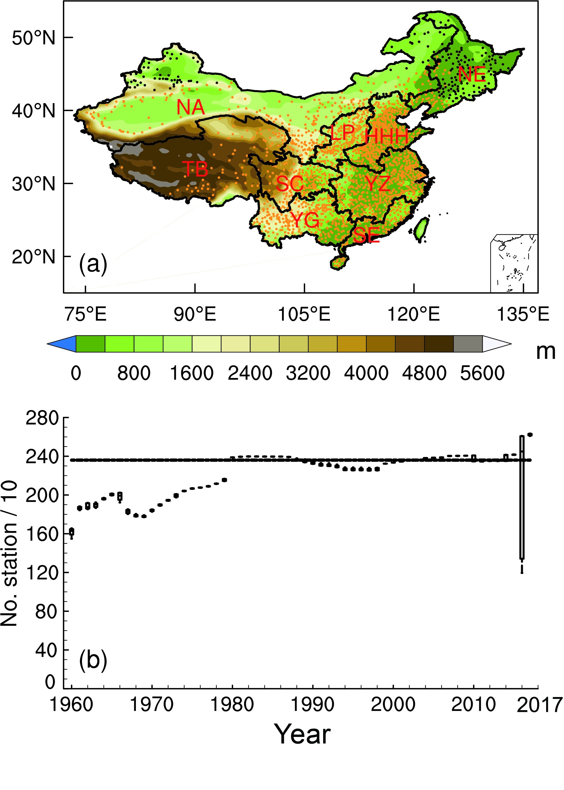 Figure1. (a) Location of the meteorological stations (dots) and the division of the nine subregions (black curves). Black dots (a total of 197 dots) denote the specific stations described in Section 3.1. (b) The number of daily stations with satisfactory data in each year. The top (bottom) of the whisker plot represents the 90th (10th) percentile of the station number, the top (bottom) of the box represents the 75th (25th) percentile, and the middle line represents the 50th percentile. The straight line indicates the final 2360 stations used in the current study (Additional information for the stations is shown in Table 1.)
To homogenize the LST dataset, several methods have been developed and applied in different countries (e.g., Hu and Feng, 2003; Zhou et al., 2017; Xu et al., 2019). Hu and Feng (2003) applied a quality-control method to the in situ soil temperature in the United States and then reproduced a high-quality soil temperature dataset at multiple soil layers. Zhou et al. (2017) applied the RHtest software package to homogenize a monthly observed LST dataset from approximately 2200 stations from 1979 to 2003 in China and then used the homogenized LST to assess eight reanalysis products. Xu et al. (2019) incorporated additional ancillary and metadata into a raw LST dataset and then constructed a homogenized monthly LST dataset from 686 meteorological stations in China. Previous studies have mainly focused on homogenizing LST datasets on monthly time scales. The daily LST can describe temporal variations at synoptic scales and is a needed parameter in weather forecasting as well as in modeling applications (Xue et al., 2012; Wu and Zhang, 2014). For instance, the daily LST from atmospheric reanalysis products has been widely used in climate research, but most of these projects underestimate the LST in China (e.g., Zhou and Wang, 2016; Zhou et al., 2017; Xu et al., 2019). Therefore, a publicly accessible homogenized and high-quality, in situ, daily LST dataset in China is urgently needed.
Since the 1980s, various methods and techniques have been developed and used to eliminate data inhomogeneities (Peterson et al., 1998; Aguilar et al., 2003; Cao and Yan, 2012). However, there is no universal homogenization method for all climatic elements across different spatial and temporal scales. Each homogenizing method has its advantages and limitations, and the choice and applicability of one method versus another are often dictated by a few influencing factors, such as the station density, availability of metadata, and the type of variable (Peterson et al., 1998). Globally, two methods are popularly used to homogenize in situ observations. One is the RHtest method (Wang et al., 2010; Wang and Feng, 2013) and the other is the Multiple Analysis of Series for Homogenization (MASH, Szentimrey, 1999, 2013, 2014). The RHtest method applies a two-phase regression model to calculate linear trends of a target time series, detect their statistically significant breakpoints, and finally, adjust them using the quantile-matching adjustment method. The MASH method uses a point-to-point comparison to detect breakpoints through an intercomparison of station observations within the same climatic area. Then, the method homogenizes the breakpoints relied on by its neighbors (a detailed description is provided in section 2.2). Because the MASH method is not overly restricted by metadata, it is widely used to homogenize meteorological variables. Li and Yan (2010) applied the MASH method to the daily air temperature of Beijing with additional reference information (with or without metadata) and found that the MASH method could successfully detect the majority of inhomogeneities in the raw dataset. For a long-term historical station observation dataset, it is usually difficult to preserve and obtain metadata (Tao et al., 1991), and this is the case for the in situ measured LST dataset in China. Nevertheless, the MASH method allows users to perform data homogenization in the case of no metadata. As a result, we select the MASH method in the present work.
In this study, we aim to develop a high-quality LST dataset that can be used in future applications for long-term climatic and soil-related researches. Using the MASH method, we examine and identify the inhomogeneities in the daily in situ collected LST from 2360 stations in the mainland of China. The manuscript is organized as follows. Section 2 describes the dataset and methods used in this study. Section 3 presents the detailed homogenization procedure. Section 4 demonstrates and discusses the changes in LST due to homogenization. The conclusions are presented in section 5.
2.1. In situ observed LST
The raw daily LST dataset from meteorological stations in China, spanning the period 1960?2017, was obtained from the National Meteorological Information Center of the China Meteorological Administration (NMIC/CMA). Fundamental quality control (e.g., screening for unreasonable extreme values) was performed on this dataset before it was released to the public (In the present work, daily LST measurements from up to 2360 meteorological stations are used. The majority of stations are located in relatively low elevation regions, which are usually densely populated (Fig. 1a). For example, there is a much higher density of stations in the Yellow River and Yangtze River basins, Southeast China, and the Central China Plain compared to other regions. The station distribution is relatively sparse in high elevations and sparsely populated areas, such as Northwest China and the Qinghai-Tibet Plateau regions. In addition, the number of effective stations (i.e., stations with measurements) was 1476 in 1960, after which it increased generally over time (stable during 1980?2010). In 2017 the number of effective stations increased to 2628 (Fig. 1b).
2
2.2. Multiple Analysis of Series for Homogenization (MASH)
The MASH method was developed by Szentimrey (1999, 2014) and is based on the hypothesis test method to detect possible breakpoints at a given significance level. Through comparisons of measurements at different stations within the same climate region, the MASH method does not require prior assumptions of a homogeneous time series. This method has been widely applied to detect and adjust the inhomogeneity of raw meteorological observations at ground stations (e.g., Li et al., 2018, 2020). Guijarro et al. (2017) tested nine commonly used homogenization methods (including the RHtest and MASH methods) and compared their homogenized performances in terms of the root mean square errors and trends of the air temperature time series. They found that the results obtained by MASH method were comparatively reliable (Guijarro et al., 2017).To homogenize daily records, the MASH method must first homogenize the corresponding monthly data. Therefore, the daily LST at each station is first aggregated to monthly values, and then, the breakpoints of the monthly LST are detected and adjusted. Finally, the MASH method is again applied to homogenize the daily LST with the incorporation of the homogenized monthly values. Detailed information of the MASH method, including the mathematics it uses and its technique, is provided in its online manual (
In the original MASH procedure, the monthly/annual value is set as missing if any missing day/month exists within that month/year. Such a strict criterion will lead to the loss of many useful records because many stations only have few days missing in a specific month. Furthermore, the loss of useful data is not the intention of data homogenization. Here, we use a lenient threshold condition for the missing value judgment to retain as many useful observation stations as possible. At each station, the monthly LST is set as a missing value when more than nine days of daily LST is missing in a given month. We also investigated the impact of different criteria (i.e., 8, 9, 10 days missing) for the count of missing months and found that there is little difference when varying criteria for a 28, 29, 30, and 31 day month. Meanwhile, the annual LST is set as a missing value when more than three continuous monthly values are missing. Finally, we remove stations with available annual values totaling less than 30 years of the full 58 years. Eventually, 2360 stations remained and were homogenized by the MASH method (shown as the straight solid line in Fig. 1b). According to the principle of MASH as well as the spatial variability of LST, we perform MASH in each individual climate region. Based on the natural conditions for agricultural production and also in consideration of climate characteristics, we divide the mainland of China into nine subregions (Fig. 1a): the Huanghe-Huaihe-Haihe Plain (HHH), Loess Plateau (LP), Middle-lower Yangtze Plain (YZ), Northeast China Plain (NE), Northern arid and semiarid region (NA), Qinghai-Tibet Plateau (TB), Sichuan Basin and surrounding regions (SC), South China (SE), and the Yunnan-Guizhou Plateau (YG). The shapefile of each subregion is available from the Institute of Geographical Sciences and Resources, Chinese Academy of Sciences (
| Full name | Abbreviation | Number of stations |
| Huanghe-Huaihe-Haihe Plain | HHH | 414 |
| Loess Plateau | LP | 202 |
| Middle-lower Yangtze Plain | YZ | 488 |
| Northeast China Plain | NE | 183 |
| Northern arid and semiarid region | NA | 328 |
| Qinghai-Tibet Plateau | TB | 90 |
| Sichuan Basin and surrounding regions | SC | 200 |
| South China | SE | 164 |
| Yunnan-Guizhou Plateau | YG | 291 |
| Mainland of China | China | 2360 |
Table1. Number of stations in each subregion
In addition, other statistical methods, including linear regression and standard deviation, are used to comparatively analyze the raw and homogenized LST dataset. A two-tailed Student’s test is used to test the significance of these statistics.
3.1. Preliminary adjustment of LSTs in northern China
As mentioned in the introduction section, automatic instruments for LST measurements began to replace manual ones in 2004 in northern China (mainly north of 40oN, including Xinjiang Province, NE, and NA subregions, shown as black dots in Fig. 1a), which resulted in LSTs increasing abruptly in cold months since 2005. To understand this result, we select one cold month (December) as an example to analyze the time series of LST over northern China. Figure 2 shows the daily LST time series averaged across 197 stations in northern China in December from 1960 to 2017. There is a distinct jump in 2005, after which the magnitude of LST increases remarkably. The mean value is –8.1oC for 2005?17, which is 8oC higher than that for 1960?2005 (–16.1oC). This phenomenon is prevalent at all 197 stations. Xu et al. (2019) found a similar problem in the same regions (the NE and NA subregions) when they compared the differences of LST measurements from manual and automatic instruments during parallel observation periods. The warm shift phenomenon is principally caused by the change of the observation system from a manual to an automatic one around 2004. In winter, when the ground surface is covered by snow, the manual instrument measures the temperature at the snow surface, whereas the automatic instrument sensor measures the temperature at the soil surface under snow. Because snow is a strong insulator of heat, it can absorb both longwave radiation from the ground surface transmitted upward and shortwave radiation from the atmosphere transmitted downward (Cohen and Rind, 1991; Groisman et al., 1994). Therefore, the measured LST from the automatic instrument would change much more slowly under snow and cannot represent real LST change features (Liu et al., 2008; Ren et al., 2013). When the manual sensor was buried in snow, it would be taken out to measure the snow surface temperature instead of the soil surface temperature (China Meteorological Administration 2003).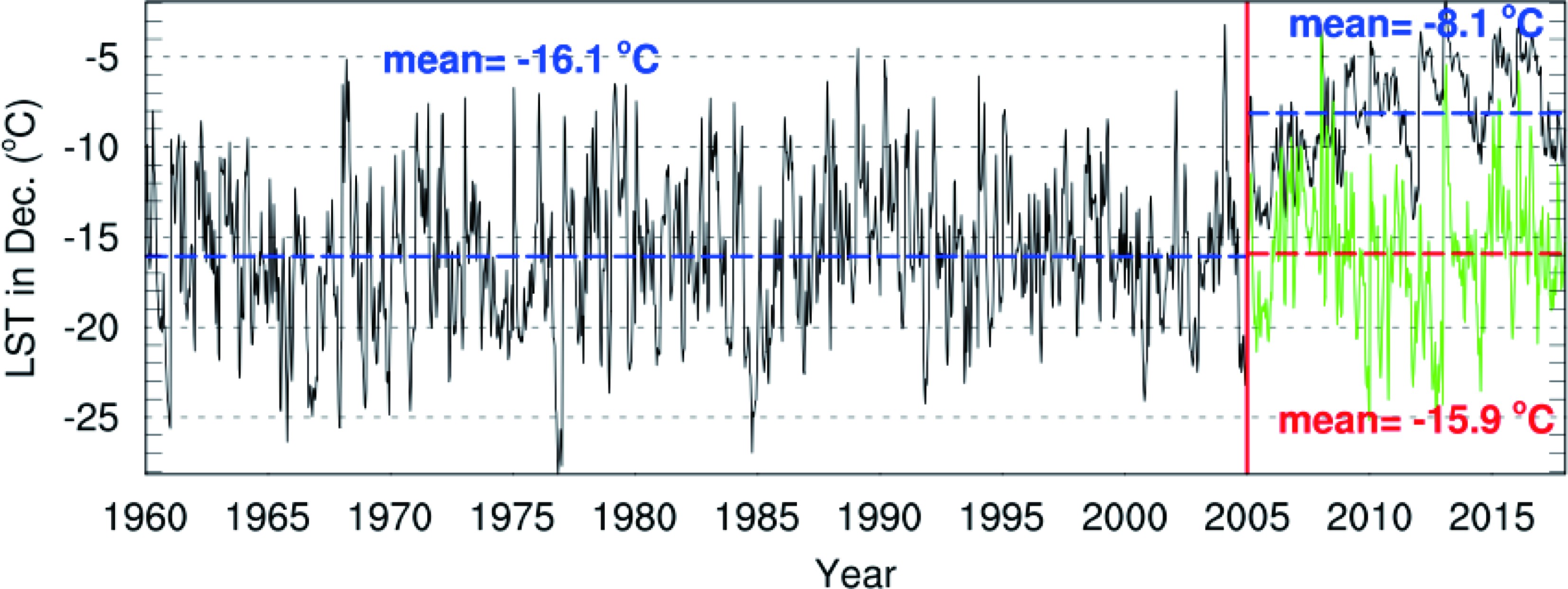 Figure2. Time series of the raw daily LST averaged across 197 stations (the black dots in Fig. 1a) in December for 1960?2017. The red solid line is a reference line to separate the years before and after 2005; the two blue dotted lines are the mean LSTs derived from the raw daily dataset during 1960?2005 and 2005?17. The green solid curve represents the daily LST time series after LSAT adjustments (section 3.1), and the red dotted line is the mean LST during 2005?17. The corresponding mean LST values averaged for different periods are also indicated.
More specifically, we take a station (ID 50862, 46.98oN, 128.05oE) at the NE subregion as an illustrative example. Figure 3 shows the abrupt warming shift in cold months (from October to the following April) since 2005. A similar phenomenon appears at all 197 stations (black dots in Fig. 1a) in the NE and NA subregions. In the MASH procedure, possible breakpoints are determined by comparing the values at the candidate station with those at the nine nearest reference stations. If those surrounding reference stations show similarly abrupt changes or shifts as the candidate station, then the MASH method cannot detect them (Li, 2016). Due to how MASH works, it will fail to deal with the specific problematic phenomenon mentioned above (compare the blue and orange lines in Fig. 3b). Thus, before applying the MASH method, we perform a preprocessing procedure for the LSTs from these 197 stations.
 Figure3. Case station (ID 50862, 46.98oN, 128.05oE) for the raw and calculated LST, and the homogenized results (units: oC). (a) Raw daily LST plotted against the calculated daily LST in each month during 1960?2004, where the black solid line is the reference (x = y) line, (b) raw (blue) and MASH homogenized (orange) daily LST, and (c) raw and calculated (green line) LST during 2003?07. The calculated daily LST is the LST adjusted by the LSAT (described in section 3.1).
There is a very close relationship between the LSAT and LST, and their differences determine surface heat fluxes (Zeng et al., 2012). The observed LSATs have undergone a strict quality control process and do not show such remarkable warming shifts. Therefore, the LSAT is used as a reference to correct the LST warming bias at each station. Simplistically and practically, it is assumed that the characteristics of the changes in LSATs are consistent with those in LSTs at the same station. This assumption is reasonable because they have a robust relationship and show similar variabilities (Vancutsem et al., 2010). The following procedure is used to adjust the LST via the LSAT. First, we construct a regression equation between the LST (dependent variable) and LSAT (independent variable) for each cold month (from October to the following April) at each of the 197 stations from 1960 to 2004. Second, the regression coefficient and the raw daily LSAT in the current month are used to compute the corresponding daily LST from 2005 to 2017. The computed LSTs are regarded as the “calculated LSTs” at the 197 stations. To verify the reasonableness and applicability of the above hypothetical relationship, we compare the raw and calculated LSTs in Fig. 3a. All the dots spread around the reference y-x line, and the monthly absolute mean differences between the calculated and raw LSTs are generally less than 1oC. In cold months, the absolute differences are less than 0.5oC, except in April (October), when there is a relatively large error in the mean differences of approximately –2oC (2oC). However, the standard deviation of the raw LST during 1960?2005 in April (October) is 3oC (6oC) and is higher than the mean difference. Therefore, it still can be concluded that the calculated LSTs are consistent with the raw LSTs during the whole period. Similar results are also shown at other stations. After the above process, the distinct warm shift of the LST in cold months is removed (Fig. 3c). The calculated daily LST across all 197 stations averaged in December from 2005 to 2017 (green line in Fig. 2) also shows consistency with the raw daily LST from 1960 to 2005, and the mean value for 2005?17 (–15.9oC) is close to that for 1961?2005 (–16.1oC). The above-calculated LSTs at 197 stations for 2005?17 are added to the raw dataset and replace the values at the same time and station.
2
3.2. Breakpoint detection by MASH
After the above preliminary adjustments, we apply the MASH method at all 2360 stations in China. The first step of MASH is to detect the temporal breakpoints of the LST time series at each station. The breakpoint (also called the change-point) is where the time series displays significant differences before and after that point. The time series shows a distinct leap at the breakpoint. To help understand this process, we take one station (ID 57710 at 27.85oN, 106.37oE) in the YG subregion as an illustrative example (Fig. 4). The LST at the candidate station (the red dot in Fig. 4a) is first compared with the values from the nine closest stations (the green dots in Fig. 4a). Compared with the other nine reference time series (Fig. 4b), a breakpoint appears in 1970 in the candidate time series, of which the mean LST during 1960?70 is 21.1oC, 3oC higher than that during 1970?2017 (18.1oC). The variability of the homogenized time series (the blue line in Fig. 4c) is akin to the nine neighbor reference time series. The time series has a warming trend [0.09oC (10 yr)–1], showing the opposite tendency compared to the raw time series [–0.26oC (10 yr)–1].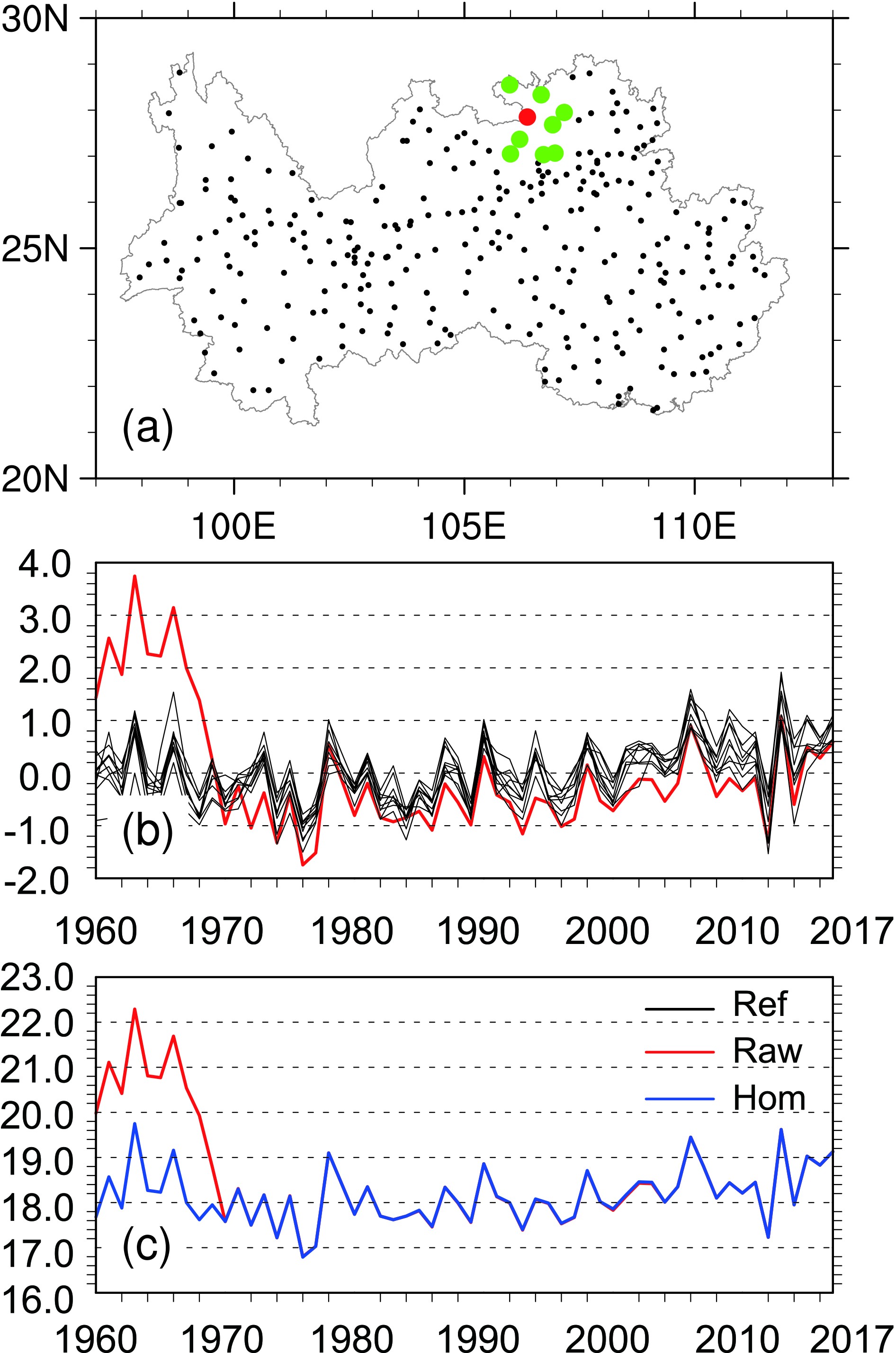 Figure4. Annual LST series at station ID 57710 (27.85oN, 106.37oE, a candidate station) in the YG subregion (units: oC). The specific information of nine reference stations is ID 57714 (27.36oN, 106.20oE), ID 57717 (27.68oN, 106.92oE), ID 57713 (27.68oN, 106.92oE), ID 57606 (28.33oN, 106.67oE), ID 57720 (27.95oN, 107.17oE), ID 57614 (28.55oN, 105.98oE), ID 57803 (27.05oN, 106.00oE), ID 57718 (27.03oN, 106.72oE), and ID 57719 (27.07oN, 106.97oE), respectively. (a) Distribution of stations, including the candidate station (red dot), the nine nearest reference stations (green dots), and other stations (black dots) in the YG subregion, (b) the raw annual LST anomalies of the candidate station (red curve) and the nine reference stations (black curves), and (c) annual LST from the raw (red curve) and homogenized time series at the candidate station.
Repeating the above procedure for all stations in each of the nine subregions, we identify the breakpoints at all 2360 stations from the monthly LST time series for 1960?2017. To better illustrate the results, we subjectively divided MASH results into two parts. The first part occurs when the absolute adjustment value is greater than 0.5oC, it is treated as the effective adjustment and its corresponding breakpoint as the effective breakpoint. The other part occurs when the absolute adjusted value is less than 0.5oC, it is regarded as the minor adjustment, in which inhomogeneity is relatively small and the MASH procedure has little effect on the time series. There are a total of 3.68 × 10³ effective breakpoints counted in Fig. 5. The plot clearly shows that the monthly LSTs at the majority of stations contain 5?25 effective breakpoints (Fig. 5). Of all 2360 stations, 35 stations contain over 40 effective breakpoints, of which most are located in the SC and SE subregions (the red dots in Fig. 5a), while 21 stations scattered across China contain no effective breakpoints (the dark blue dots in Fig. 5a). The effective breakpoints are relatively concentrated in the SE, HHH, and SC subregions, where there are at least 20 effective breakpoints identified in most stations. Having aggregated the numbers of effective breakpoints at all stations (Fig. 5b), nearly 500 effective breakpoints occur each year on average. However, the number of effective breakpoints shows distinct interannual variations and evidently increases over time, in particular since 2000. In 2003, when the replacement of the LST measurement instruments occurred at many stations throughout China, more than 1200 effective breakpoints are identified. At this time, the number of effective breakpoints reaches its maximum value. For the monthly LST time series, the number of effective breakpoints in cold months (January to April, and November to December) is higher than in warm months (May to September) in every year. Previous documents and reports have also mentioned that the LST measurement instruments used for in situ observation systems have been gradually changed from manual to automatic ones since 2000 (Liu et al., 2008; Xu et al., 2019). Furthermore, it is well known that urbanization has developed rapidly during recent decades in China. The fact that some stations suffered from changes in the surrounding environment may also induce abrupt changes in the LST records, which is another reason for the increase in the number of breakpoints (Yan et al., 2010).
 Figure5. The number of effective breakpoints for the monthly LST records at the effective stations during 1960?2017; (a) the spatial distribution at all stations and (b) the accumulation in each month and each year across all stations.
2
3.3. Frequency distribution of adjustments in MASH
To explore the LST adjustments identified in the MASH procedure, we count the number of effective breakpoints at all stations in each subregion and throughout the mainland of China. There are approximately 1.6 × 10⁶ monthly records, of which 3.28 × 10⁵ records (approximately 20% of the total records) show effective adjustments in MASH. In each subregion (Fig. 6), the majority of effective adjustments vary between 0.5oC and 1.5oC and between –0.5oC and –1.5oC (2.95 × 10⁵ or 90% of all effective adjustments), within which two peaks are found around 0.5oC to 1.0oC and –0.5oC to –1.0oC. Except for the TB subregion, stations in other subregions show that the number of effective breakpoints with positive adjustments is greater than the number with negative ones. Moreover, minor adjustments are also counted in Fig. 7. We find that the minor adjustments account for 80% of the total adjustments in most subregions and in all of the mainland of China, which is consistent with the above results (effective adjustments records account for approximately 20% of the total records). Obviously, the percentage of minor adjustments in the SE subregion between July and October is low (less than 60%, red line with an inverted triangle in Fig. 7). This indicates that the percentage of effective adjustments in SE subregion is relatively large (over 40%). Except for the SE subregion, the YZ (NE) subregion in the cold season shows the highest (lowest) percentage of minor adjustments, above 90% (below 80%). Approximately 80% of the total records in the HHH subregion have experienced minor adjustments. Considering the large variability of the daily data, it is difficult to directly homogenize the daily time series. Therefore, MASH identifies the inhomogeneities from the monthly time series and applies the result to estimate the inhomogeneities of daily time series through smooth interpolation. We also plotted the frequency distribution of daily adjusted records (figures not shown) and it indeed exhibits similar characteristics with the monthly results. Figure6. Frequency distribution for the effective breakpoints of LST in the nine subregions and for the whole of the Chinese mainland. Biases at these breakpoints are adjusted with MASH.
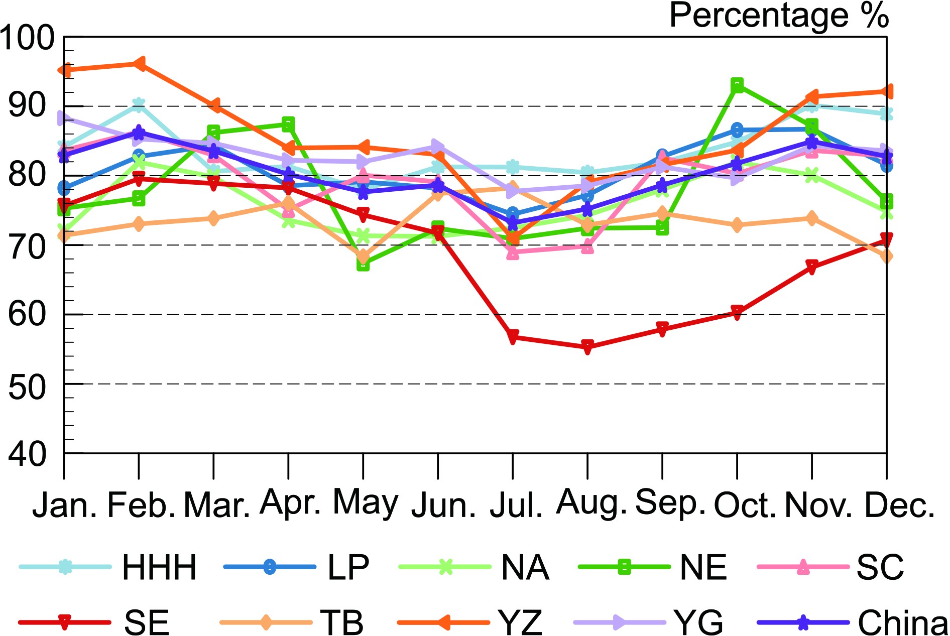 Figure7. Percentage of records with adjusted LST biases between –0.5oC and 0.5oC in different months over the nine subregions and the whole of the Chinese mainland.
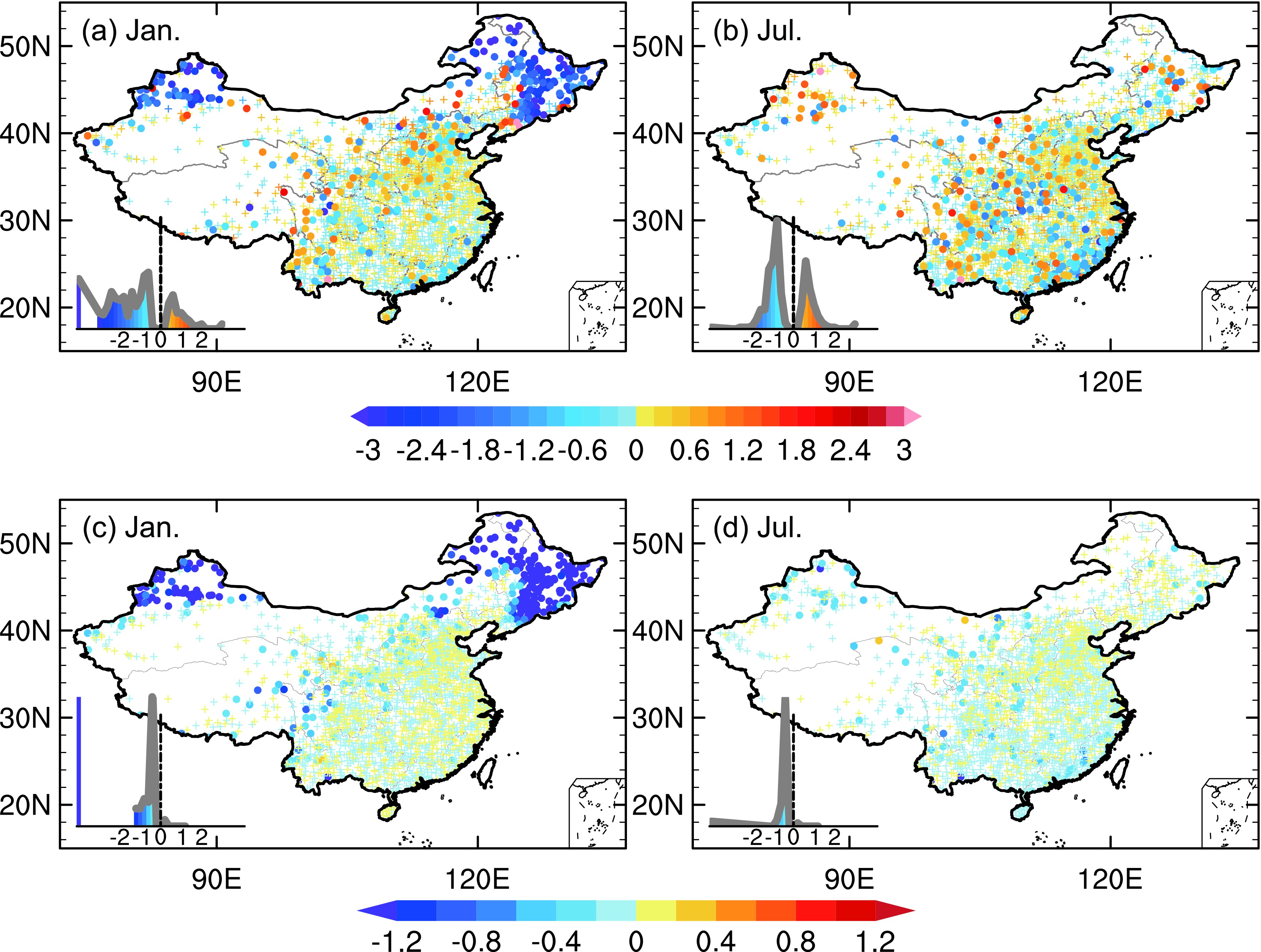 Figure8. Spatial distribution of the differences of the monthly means [(a), (b)] and standard deviations [(c), (d)] between the homogenized and raw LSTs in January [(a), (c)] and July [(b), (d)] (units: oC). The filled dot and the “+” symbol indicate the mean LST differences passing or not passing the significance test (p = 0.05), respectively. The histogram plot in the lower-left corner shows the frequency distribution of the significant differences.
In winter, 81 (279) stations display significantly positive (negative) differences (p = 0.05) between the homogenized and raw monthly mean LSTs (Fig. 8a). Among these stations, 163 (58% of 279) stations with significantly negative differences are located north of 40oN, while some are in the SE subregion. In summer, stations with significant LST differences are relatively concentrated in the YG, SC, SE, and NA subregions (Fig. 8b), where 325 stations had significant LST differences, of which 117 (208) stations showed positive (negative) differences. In both winter and summer, the significant negative differences generally vary between –2oC and –1oC, while the significant positive differences are within 1oC (histogram plots in Figs. 8a, b).
We use the standard deviation to represent the interannual variability, and its difference between homogenized and raw data can be regarded as the changes of the interannual variability of LST. In winter, the interannual variability of the homogenized monthly LST is much smaller than that of the raw values (Fig. 8c). All 197 stations north of 40oN (Fig. 1a) show negative differences. Stations with negative differences are also prevalent in the TB subregion. In summer (Fig. 8d), the interannual variability of the homogenized mean exhibits a remarkable difference from that of the raw mean at 102 stations, of which 100 stations display negative differences, which indicates that our homogenization process reduces the interannual variability remarkably at most stations for both winter or summer.
To explore the changes in the long-term tendency of LST due to the MASH process, we also computed the linear trend for the homogenized and raw LSTs at all 2360 stations in winter and summer during 1960?2017. In winter (Figs. 9a, b), 144 stations (6% of all 2360 stations) have negative linear trends in the raw dataset, of which only the trends at three stations are significant (p =0.05). Most stations show positive trends (94% of all 2360 stations), of which the LST trend at 57% of stations is significant (p =0.05). Stations with significant positive LST trends are concentrated in the NA, NE, LP, HHH, and TB subregions, and stations with negative trends are mainly located in the YG and YZ subregions. After homogenization, the number of stations with negative trends decreases from 144 to 45, and the LST trends at all these stations are not significant. The percentage of stations with significant positive LST trends (57%) does not change, but the distribution differs greatly. Compared to the linear trend of raw LSTs, stations with significant positive trends are reduced north of 40oN (the NE subregion and Xinjiang Province) but increase in the SE and TB subregions. In summer (Figs. 9c, d), stations with negative trends increase and occupy almost the entire southern part of the Yellow River Basin. There are in total 648 stations with negative trends and 12% of these are significant for the raw LSTs. This number increases to 659, while only 2% of them are significant for the homogenized LSTs, indicating that the homogenization process reduces the LST trends overall in the mainland of China.
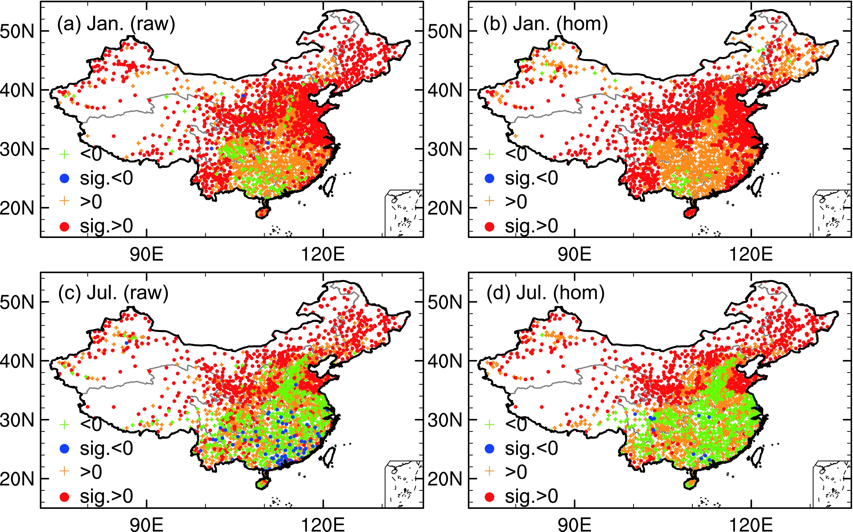 Figure9. Distribution of linear trends of the monthly raw and homogenized LST in January [(a), (b)] and July [(c), (d)]. The filled dot (“+”) indicates stations with trends passing (not passing) the significance test (p = 0.05).
Finally, we perform a preliminary analysis of the homogenized LST dataset in terms of its temporal and spatial variations. Figure 10 displays the distribution of the annual mean homogenized LST and its time series averaged in China. It is worth mentioning that the number of missing measurements in 2016 is relatively large (also seen in Fig. 1b), in particular to the south of the Yellow River basin. Therefore, the mean value in 2016 is given as missing. Notably, the annual mean LST has below zero degrees Celsius at very few stations distributed in the NE subregion, while most stations show positive values. Moreover, for the entire period of 1960?2017, the annual mean LST shows a significant warming trend of approximately 0.22oC (10 yr)–1, which is consistent with previous studies (Zhou et al., 2017; Xu et al., 2019). The trend of the annual mean LSAT shows a similar magnitude [0.21oC (10 yr)–1], and the annual mean LST is generally 2oC higher than the annual mean LSAT.
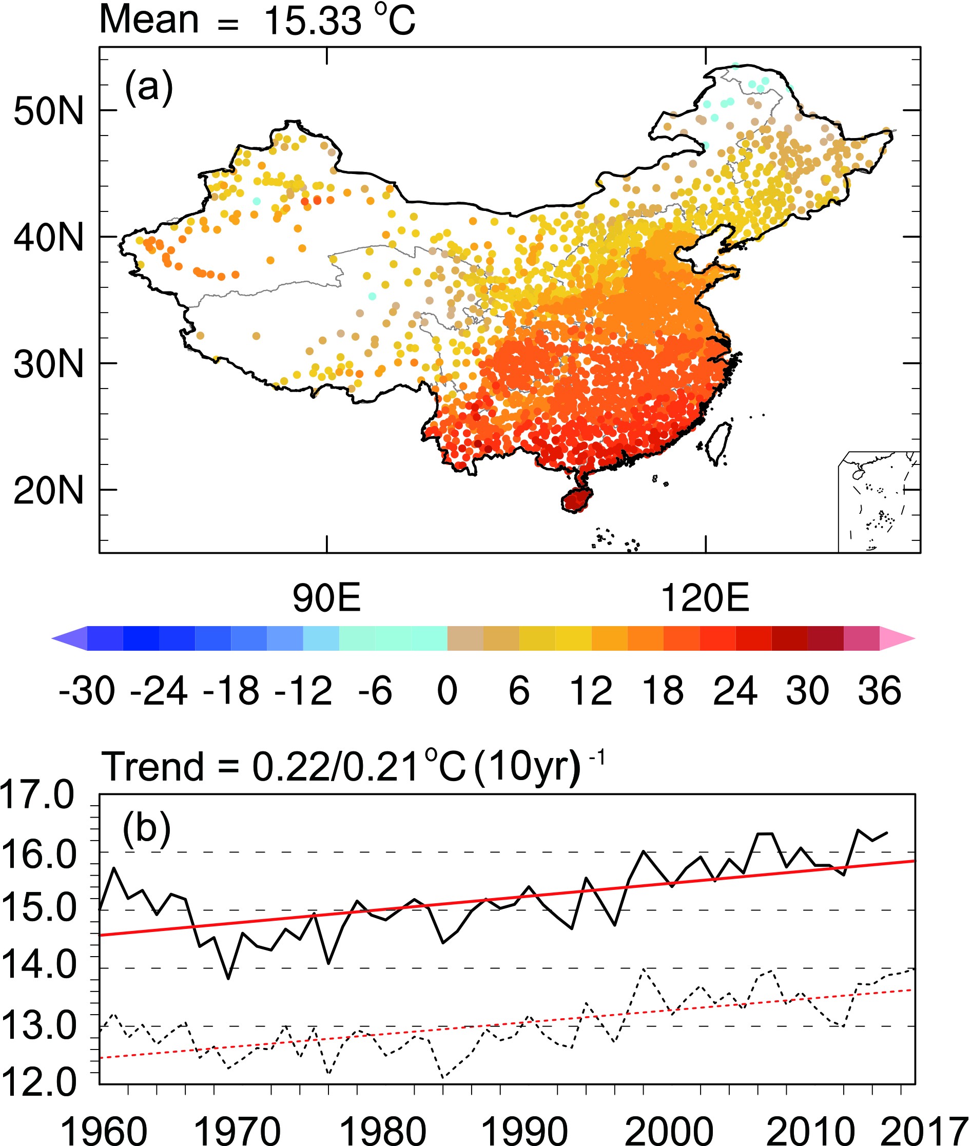 Figure10. (a) Distribution of the multiyear mean homogenized LST and (b) its time series and linear trend averaged over all stations in China (LST/LSAT with the solid line/dotted line) for 1960?2017 (units: oC).
Due to the replacement of instruments from manual to automatic ones around 2004 north of 40oN, the time series of the LSTs at 197 stations display remarkable warming shifts during cold months. This warming bias fails to be homogenized by the MASH method. Therefore, the raw LST records at the above stations are first adjusted using the high-quality LSAT under the assumption of the same monthly variability of both the LST and LSAT at the same station.
Then, the MASH method is applied to homogenize the LST dataset in China. During 1960?2017, 5?25 significant breakpoints are detected in the LST monthly time series at most stations. Stations in southern China and most parts of the Sichuan Basin exhibited more intensive breakpoints than those in other subregions. The number of breakpoints has increased since 2000. Notably, in 2004, breakpoints are detected at more than 1200 stations. For most breakpoints, the absolute adjusted biases due to MASH are between 0.5oC and 1.5oC, with peaks around 0.5oC and –0.5oC. Moreover, comparing the difference between the homogenized and raw LSTs, the MASH process generally reduces the magnitude, interannual variability, and linear trends of LST. The interannual variabilities and linear trends of the homogenized LSTs are also reduced at the majority of stations, especially in the regions north of 40oN in winter.
It should be noted that there are some limitations of the new homogenized LST dataset north of 40oN. We preliminarily adjusted warm shifts of LSTs in cold seasons from 2005 onwards simply by using a linear relationship between the LST and LSAT, but many other factors can also directly affect changes in LST, including precipitation frequency, solar radiation, vegetation growth, surface roughness (Zeng et al., 2012; Zhou et al., 2017). In a recently published article, Du et al. (2020) corrected LSTs through LSATs while considering the influences of snow depth and solar radiation. They found that the LST-LSAT relationship is stable and near-linear under snow-free conditions, but that it is sensitive to both snow depth and solar radiation. Therefore, the above uncertainty should be considered when this dataset is applied in further research.
In summary, we provide a 58-year (1960?2017) homogenized daily LST dataset with an abundant number of stations (2360) in China. The current paper only presents the homogenization process of the LST dataset and some preliminary analyses for LSTs, but our work extends beyond this. We have applied the MASH method to soil temperature at six soil depths (0 cm, 5 cm, 10 cm, 15 cm, 20 cm, and 40 cm). The results for soil temperatures in other soil depths are similar to those for LST, so we do not present them in this paper. The long-term homogenized LST and soil temperature in multiple soil depths contain a relatively dense number of stations and can have a variety of applications, such as for model evaluation and climate and soil-related research.
Acknowledgements. This work was supported by the National Science Fund for Distinguished Young Scholars (Grant No. 41925021) and the National Natural Science Foundation of China (Grant No. 41875106). The new homogenized daily LST dataset in this research is available from the authors for various applications.
