HTML
--> --> -->However, record breaking Arctic ozone loss was observed in spring 2020 (Dameris et al., 2020; Hu, 2020; Lawrence et al., 2020; Manney et al., 2020; Rao and Garfinkel, 2020). It is known that ozone-depleting substances have been declining since the late 1990s, and the Antarctic ozone hole and global ozone have been slowly recovering in the past two decades (WMO, 2018), which has slightly reversed the trends in tropospheric circulation (Xia et al., 2020). Recent studies have demonstrated that ozone loss in spring 2020 was closely related to the extremely strong and cold polar vortex which was caused by unusually weak tropospheric wave activities (Hu, 2020; Lawrence et al., 2020; Manney et al., 2020; Rao and Garfinkel, 2020). Thus, it is of great interest to determine what caused the unusually weak tropospheric wave activities.
In the present work, we first briefly show observational results of the extreme Arctic ozone loss in spring 2020 and associated characteristics of the Arctic stratospheric vortex. Next, we analyze how the extremely cold polar vortex is related to anomalously weak wave activity and how the weak wave activity is related to warm sea surface temperature (SST) anomalies in the North Pacific. Then, we perform model simulations to verify that warm SST anomalies in the North Pacific are likely the major factor in causing the cold Arctic stratospheric polar vortex and severe ozone loss through weakening planetary wave activities.
The model used in this study is the Whole Atmosphere Community Climate Model version 5 (WACCM5). The WACCM5 is a fully coupled chemistry climate model [see Garcia et al. (2007), and references therein]. It extends from the surface to the lower thermosphere (~145 km or 4.5 × 10?6 hPa) with 66 vertical levels. The horizontal resolution is 1.9o × 2.5o in latitude and longitude. Here, we use the WACCM5 compiled from the Community Earth System Model version 1.2 (CESM 1.2).
To investigate the impact of the North Pacific warm SST anomalies on the Arctic stratospheric vortex, we first perform a simulation for 50 years to reach the equilibrium state with greenhouse gases, aerosols, solar constant, sea ice, and chlorofluorocarbons (CFCs) all at the year-2000 values (case F_2000_WACCM5). SSTs are prescribed with the observed climatological monthly mean SSTs over 1982–2001.
Then, we perform two sets of ensemble simulations, using the equilibrium simulation results as initial conditions. For the set of control simulations, SSTs are the same climatological mean over 1982–2001. For the set of sensitivity simulations, North Pacific SST anomalies within the region of 150oE–130oW and 25o–50oN from January to April 2020 are added to the climatological mean SSTs over 1982–2001, and all other conditions are the same as those in the control simulations. Both control and sensitivity simulations have 20 ensemble members with small perturbations for the initial condition, and all simulations start from 1 January and end on 31 December. Comparison of the ensemble means between the sensitivity and control simulations reflects responses of Arctic ozone and meteorological variables to warm SST anomalies in the North Pacific.
3.1. Extreme Arctic ozone loss in spring 2020
Figure 1 shows the time series of Arctic total column ozone and associated meteorological variables from November 2019 to April 2020 (red lines). For comparison, time series of these variables are also plotted from the period 2010–11 (blue lines), which includes the second most severe example of ozone depletion in the Arctic. Overall, the polar-mean total column ozone shows that record-low values occurred from middle February to late April of 2020 (Fig. 1a). Figure 1b shows the time series of minimum total column ozone within the polar cap. Record-low total column ozone persisted from 3 March to 24 April and was lower than the Antarctic ozone hole threshold of 220 DU. The lowest value was 205 DU, occurring on 12 March. The time series of severe ozone depletion in spring 2011 is similar to the case in spring 2020, except that the polar-mean total column ozone in 2011 returned to the climatological mean level in early April, and it did not reach the Antarctic ozone hole threshold (Hurwitz et al., 2011; Manney et al., 2011; Hu and Xia, 2013).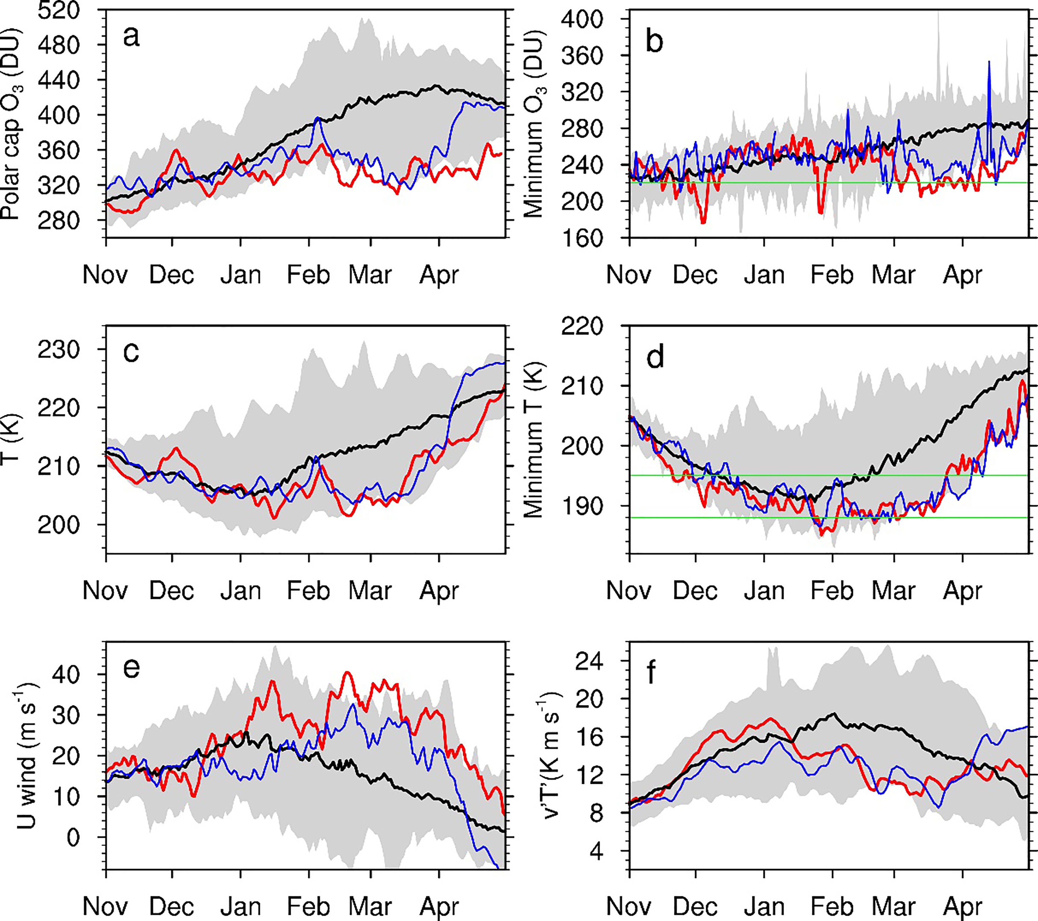 Figure1. Time series of daily Arctic total column ozone and associated meteorological variables from 1 November 2019 to 30 April 2020. (a) Total column ozone area-weighted over 63°–90°N, (b) minimum total column ozone within the polar cap, (c) temperature area-weighted over 60°–90°N at 50 hPa, (d) minimum temperatures at 50 hPa within the polar cap, (e) zonal-mean zonal winds at 60°N and 50 hPa, and (f) eddy-heat fluxes area-weighted from 45°–75°N at 150 hPa and averaged for the 45-day period prior to the date indicated. In all plots, red lines are for 2019–20, the black lines are for the climatological mean, the blue lines are for 2010–11, and grey shading denotes the daily maximum and minimum values over 1980–2019. The green line in (b) marks the threshold of the ozone hole (220 DU). The green lines in (d) mark the temperature thresholds for Type-I (195 K) and Type-II (188 K) PSCs formation.
Severe ozone depletion in the Arctic stratosphere is closely related to extremely low temperatures which cause the formation of PSCs and lead to heterogeneous and catalytic chemical reactions. Figures 1c–d show the time series of the polar-mean temperatures and the minimum temperatures at 50 hPa within the polar cap. The polar-mean temperature remained at record-low values from middle February to middle March 2020 (Fig. 1c). Record-low polar minimum temperatures persisted from 1 March to 23 March (Fig. 1d), and the lowest minimum temperatures were even lower than the threshold for Type-II PSC formation (188 K) in late February and early March. The polar-mean and polar minimum temperatures in spring 2011 were similar to those in spring 2020, except that the polar-mean temperature in 2011 increased rapidly in early April. These results indicate that severe ozone depletion in the Arctic stratosphere in both 2020 and 2011 was associated with extremely low polar temperatures.
Consistent with anomalously low polar temperatures, the polar night jet was also anomalously strong over February–April (Fig. 1e). In particular, the polar night jet reached record-high speeds of 38 m s-1 over 15 February to 13 March. For the case of 2011, the polar night jet was also persistently strong from February to early April but was weaker than that in 2020. The strong polar night jet in the stratosphere isolated ozone-poor polar air from surrounding ozone-rich air. This helped maintain the severe ozone loss inside the polar vortex.
Polar stratospheric temperatures are determined by both radiative and dynamical processes (Andrews et al., 1987; Hu and Tung, 2002). In the winter season, variations of polar stratospheric temperatures are dominated by wave-driven dynamic heating. Strong planetary wave activity can cause rapid increases in polar stratospheric temperatures, and vice versa. Figure 1f shows eddy heat fluxes at 150 hPa averaged over 45°–75°N, which approximately represents wave activity propagating from the troposphere into the stratosphere. Eddy heat fluxes started decreasing from middle January 2020 and persisted until the end of March. Eddy heat fluxes were especially weak from middle February to middle March and reached a record-low value in late February. Similarly, eddy heat fluxes in 2011 were also anomalously weak, even weaker than those in 2020 over December–January, but increased rapidly in late March.
The above results indicate that severe Arctic ozone loss in spring of both 2020 and 2011 was associated with anomalously weak wave activity and its extended persistence. It is the anomalously weak wave activity that caused the extremely cold and stable Arctic stratospheric polar vortex and consequently favored extreme Arctic ozone loss in spring. The difference between the two cases is that polar temperatures in 2011 returned to normal values earlier, so that no further ozone depletion occurred. This is probably the reason why total column ozone in spring 2011 did not reach the ozone hole threshold.
Note that positive feedbacks are likely involved in severe ozone depletion in spring 2020 and 2011 (Randel and Wu, 1999; Hu and Tung, 2003; Lawrence et al., 2020). That is, weak wave activity leads to the cold vortex and severe ozone depletion. Then, less absorption of ultraviolet radiation in spring causes a much colder polar vortex. As a result, more PSCs are formed, and more ozone is depleted. The anomalously strong polar night jet also reflects planetary waves from the troposphere, which in turn causes a colder and stronger Arctic stratospheric vortex and more severe ozone depletion.
2
3.2. Anomalously weak wave activities and their linkage to North Pacific SSTs
To identify why tropospheric wave activities were so weak in February and March 2020, we examine the possible factors that have important influences on tropospheric wave activities, including the El Ni?o–Southern Oscillation (ENSO) (Hamilton, 1993; García-Herrera et al., 2006; Calvo et al., 2008; Garfinkel and Hartmann, 2008; Xie et al., 2012; Domeisen et al., 2019) and the quasi-biennial oscillation (QBO) (Holton and Tan, 1980; Anstey and Shepherd, 2014). However, there were only moderately warm tropical SST anomalies in the winter of 2019/20 (see details atRecent studies have suggested that Arctic sea ice loss, especially over the Barents–Kara seas, enhances the upward propagation of planetary-scale waves and subsequently weakens the stratospheric polar vortex in winter (Kim et al., 2014; García-Serrano et al., 2015; Nakamura et al., 2015; King et al., 2016). Further studies have demonstrated that Arctic sea ice loss in different regions leads to contrasting impacts on the stratospheric polar vortex (Sun et al., 2015; McKenna et al., 2018). Sea ice loss in the Atlantic sector of the Arctic (Barents–Kara seas) may result in a weakening of the stratospheric polar vortex in winter and a strengthening of the vortex in spring, while sea ice loss in the Pacific sector (Chukchi–Bering seas) may lead to a strengthening of the Arctic stratospheric vortex in winter. Blackport and Screen (2019) argued that the response of winter atmospheric circulation to sea ice loss is primarily driven by sea ice loss in winter rather than in autumn. Our own analysis indicates that there was Arctic sea ice loss only in the Pacific sector in the summer and autumn of 2019, but little sea ice loss from December 2019 to March 2020. Therefore, Arctic sea ice loss seems not to be an important factor in causing the weakening of planetary wave activity either.
Several recent studies have suggested that SSTs in the North Pacific have important influences on the Arctic stratospheric vortex in NH winter and spring seasons (Jadin et al., 2010; Hurwitz et al., 2012; Woo et al., 2015; Hu et al., 2018). These works have shown that warm SST anomalies in the North Pacific tend to weaken the Aleutian low and tropospheric planetary wave activity, which consequently causes an anomalously strong stratospheric Arctic vortex. Following these studies, we examine whether North Pacific SST anomalies in the winter and spring of 2019/20 have significant effects on the Arctic stratospheric vortex and the record ozone loss.
Figures 2a–c show SST anomalies in the NH for January, February, and March 2020. A band of warm SST anomalies is located in the North Pacific approximately between 30°N and 45°N. The warm SST anomalies have two centers, with one center at 150°W and 40°N and the other one in the east of Japan. The maximum SST anomaly is about 2°C. The time series of SST anomalies averaged in the domain enclosed by the white box (30°–45°N and 150°E–130°W) shows record-high values persisting from late February to the end of April (Fig. 3).
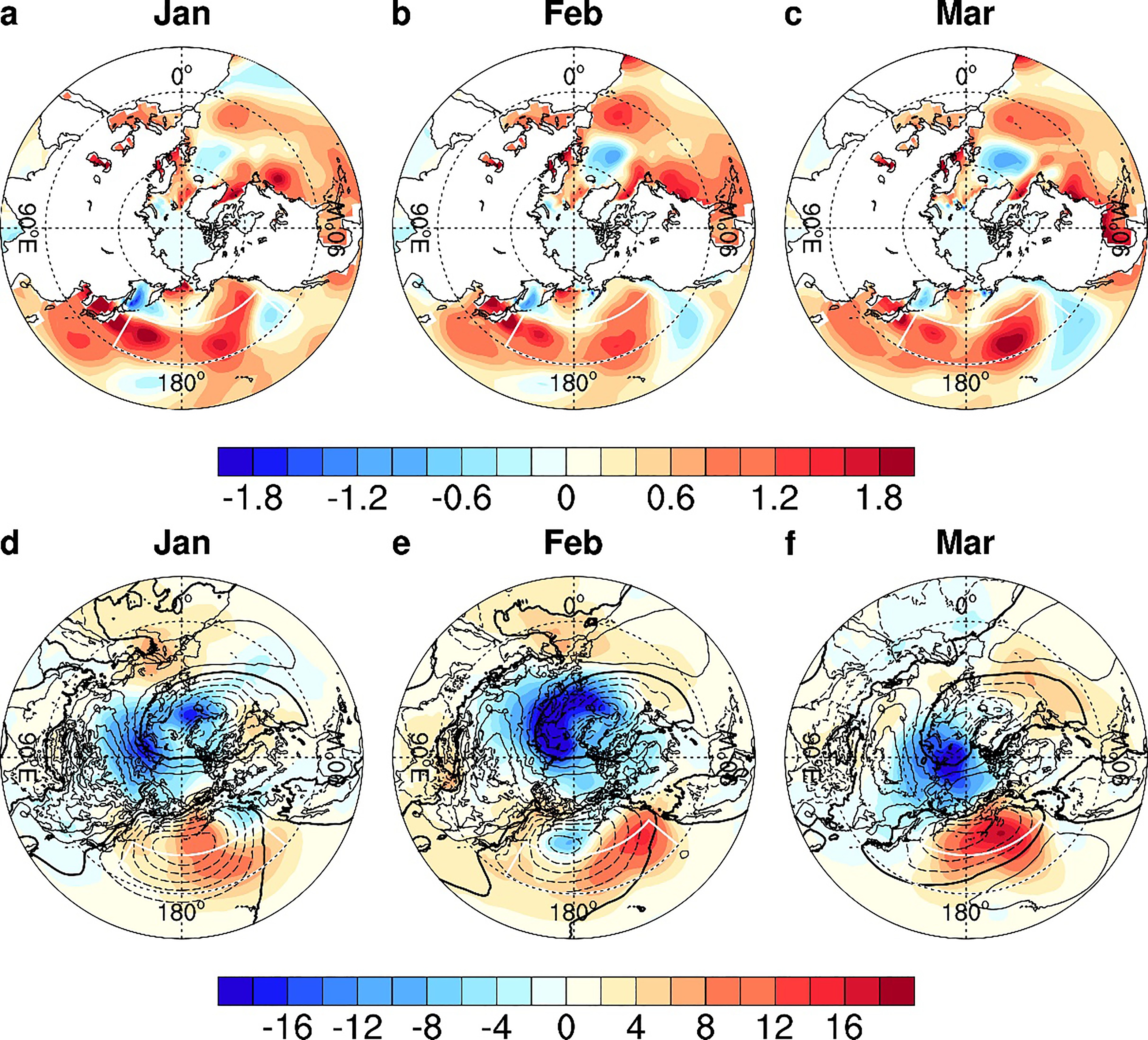 Figure2. Distributions of SST anomalies in the North Pacific and associated SLP anomalies in January, February, and March 2020. (a–c) SST anomalies with color interval of 0.2°C, and (d–f) SLP anomalies (color shading with color interval of 2.0 hPa). The contours in (d–f) denote the climatological mean SLP, with the zonal-mean removed. White boxes indicate the area of warm SST anomalies in the area of 30°–45°N and 150°E–130°W.
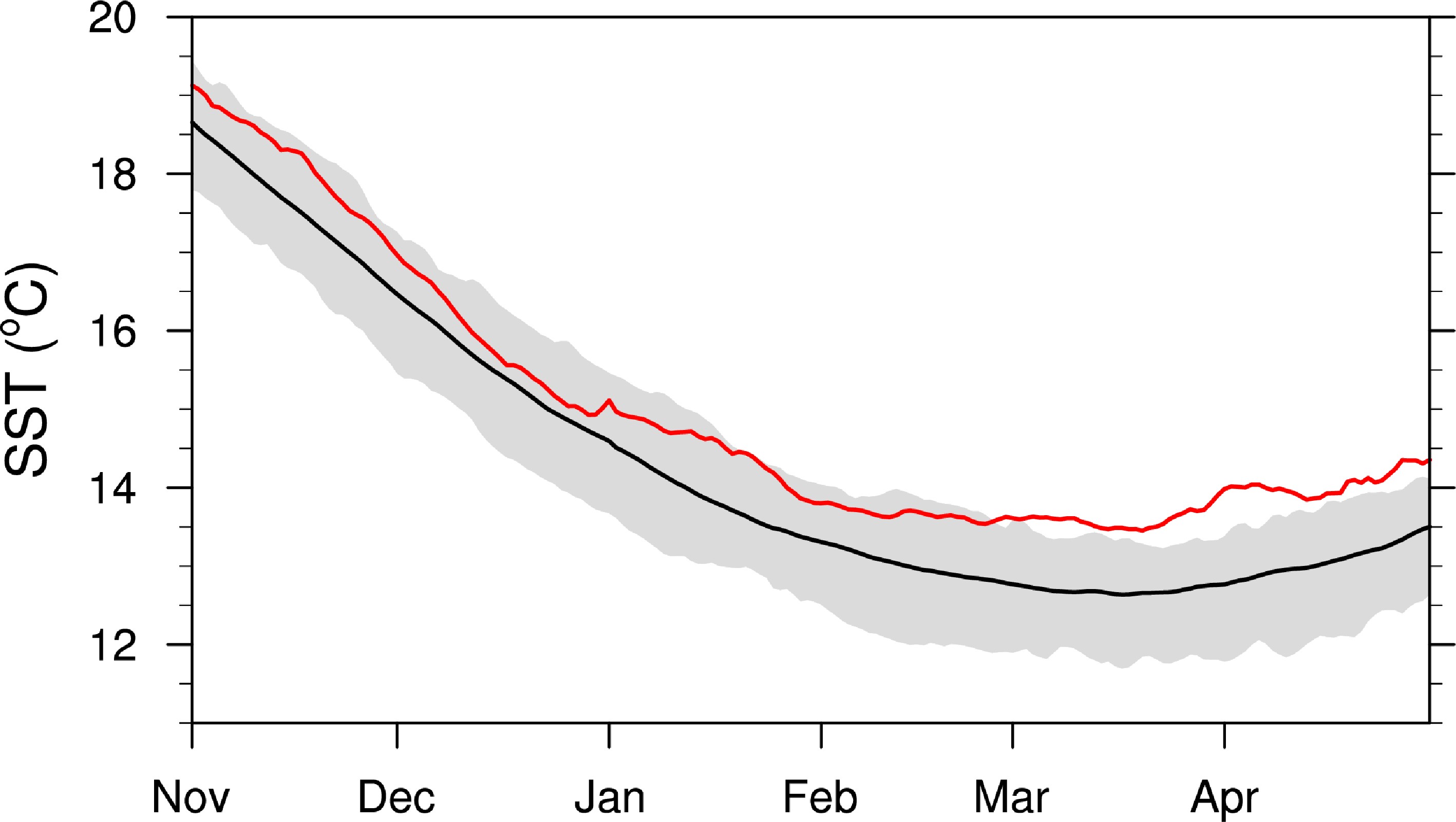 Figure3. Time series of daily SSTs averaged over the white box in Fig. 2 (30°–45°N and 150oE–130oW) from November to April. The black line is the climatological mean SST over 1982–2019 in the same region, and the red line is daily SSTs for 2019–20. The grey shading denotes the range between the minimum and maximum SSTs over 1982–2019.
Associated with North Pacific warm SST anomalies, sea level pressure (SLP) increases over the North Pacific (Figs. 2d–f), which indicate weakening of the Aleutian low, are illustrated with dashed contours. Correlation coefficients between SLP and SST averaged within the white box are significantly positive over the North Pacific (Figs. 4a–c). The maximum correlation coefficients for January, February, and March are about 0.50, 0.49, and 0.63, respectively. This suggests that the weakening of the Aleutian low is indeed closely related to the warm North Pacific SST anomalies.
 Figure4. Distributions of correlation coefficients between averaged SSTs over 30°–45°N and 150°E–130°W (blue boxes) and (a–c) sea level pressure (SLP) and geopotential height at (d–f) 500 hPa and (g–i) 150 hPa over 1980–2019 in January, February, and March. Color shading denotes correlation coefficients. Black contours denote the climatological mean SLP and geopotential heights, with the zonal mean removed. Dotted areas are the regions that have statistical significance above the 95 % confidence level (student’s t-test).
The geopotential height anomalies in the North Pacific are not limited to the surface, but they extend to higher levels. The anomalies and climatological mean of geopotential heights at 500 hPa and 150 hPa in January–March 2020 are shown in Fig. 5. Positive geopotential height anomalies are found in the extratropics. The positive anomalies in the extratropics are not zonally uniform, but exhibit wave-like patterns. At both 500 hPa and 150 hPa, positive anomalies are mainly located over the North Pacific, which indicates a weakening and westward shift of the Asian trough. Correlation analysis demonstrates that the positive geopotential height anomalies in the North Pacific are significantly correlated with the North Pacific warming (Figs. 4d–i). In the following, we show how the geopotential height anomalies interfere with the climatological mean patterns of planetary waves and cause changes in amplitudes of planetary waves in February and March 2020.
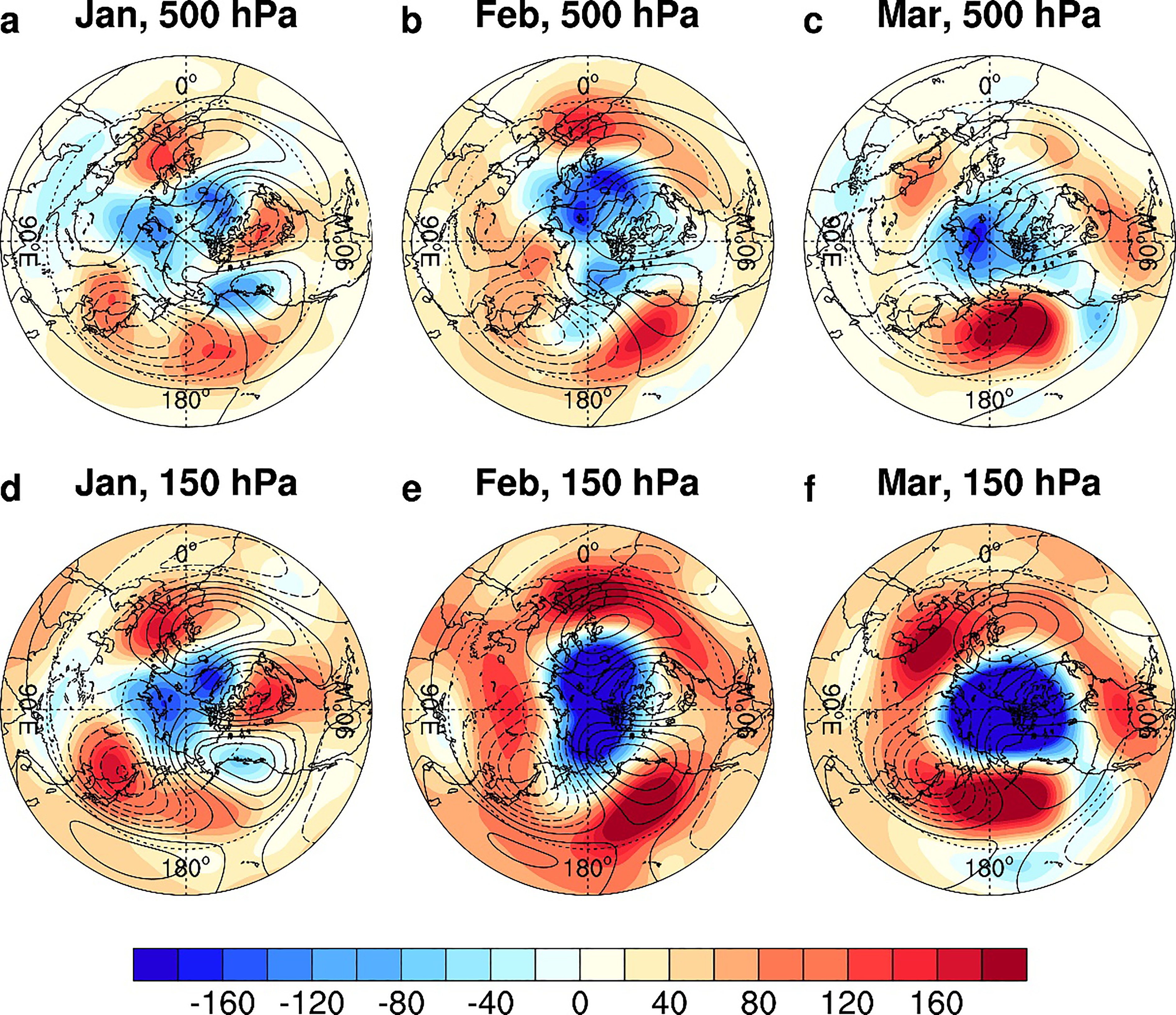 Figure5. Distributions of geopotential height anomalies (color shading) in January, February, and March 2020 at (a–c) 500 hPa and (d–f) 150 hPa. Color interval is 20 m. Black contours denote the climatological mean geopotential heights, with the zonal mean removed.
Figure 6 shows longitude-height cross-sections of wavenumber-1 and wavenumber-2 components of geopotential height anomalies in February and March 2020. First, both waves show westward tilting with altitude. Second, comparison between the climatological mean anomalies (contours) indicates that the wavenumber-1 component is largely reduced at all levels because negative and positive anomalies overlap the climatological mean ridge and trough, respectively, especially in March (Fig. 6b). The reduction of wavenumber-1 wave amplitude increases with altitude. The largest reduction is greater than 250 m at 20 hPa and 10 hPa. In contrast, wavenumber-2 wave activity is intensified. The largest increase of wavenumber-2 wave amplitude is about 140 m in March. Overall, planetary wave activity is weakened in February and March 2020 because of the dominance of the wavenumber-1 wave activity.
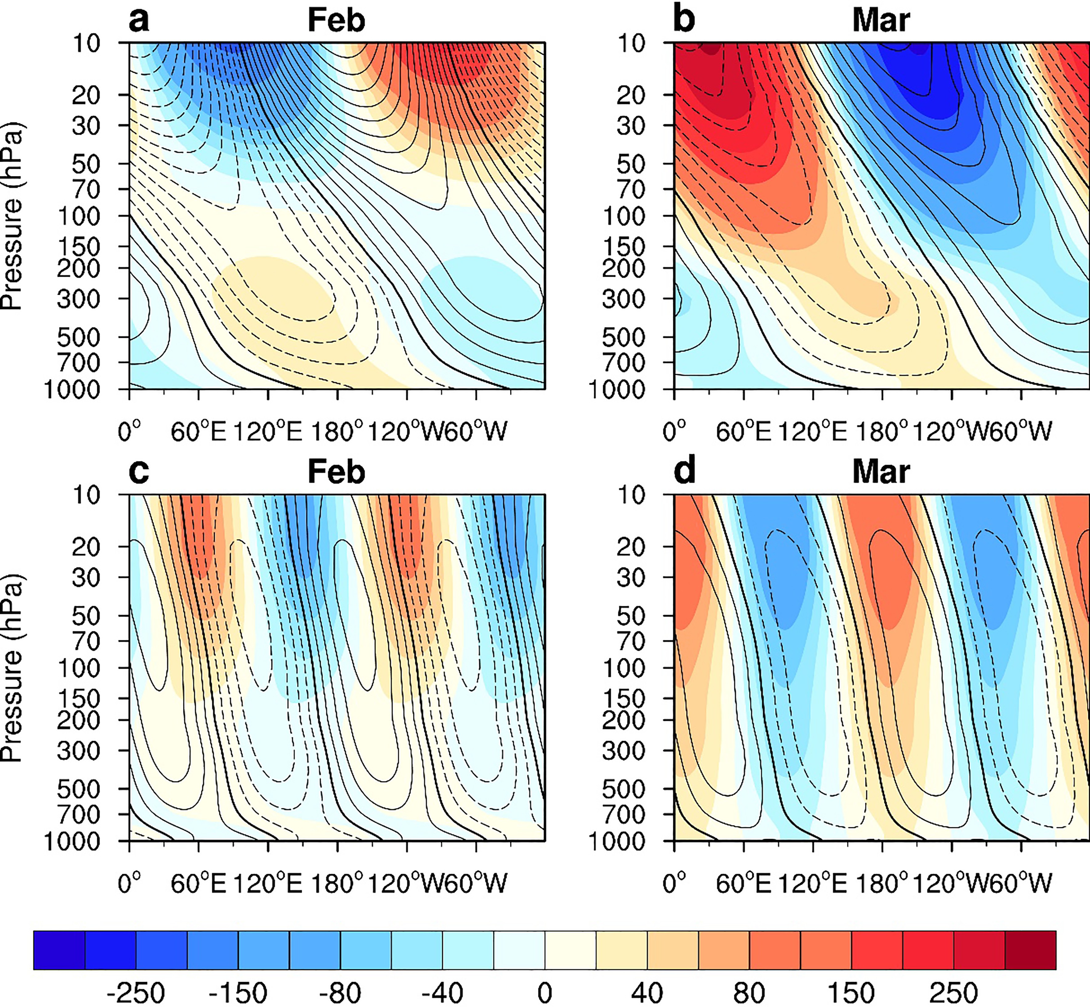 Figure6. Longitude-height sections of geopotential height anomalies decomposed into wavenumber-1 and wavenumber-2 components averaged between 30°N and 70°N in February and March. Upper panels: (a–b) wavenumber-1, and lower panels: (c–d) wavenumber-2. Black contours indicate the decomposition of climatological mean geopotential height anomalies. Solid contours denote positive geopotential height anomalies, and dashed contours denote negative geopotential height anomalies. Color shading denotes decomposition of geopotential height anomalies in 2020. The color interval is 20 m.
The above results indicate that the weakening of wavenumber-1 wave activity, which is responsible for the extremely cold Arctic stratospheric vortex, is associated with the warm SST anomalies in the North Pacific in February and March 2020. Similar results can also be found in the European Centre for Medium-range Weather Forecasts Reanalysis 5 (ERA5). The results are consistent with previous studies that warm SST anomalies in the North Pacific result in a weaker Aleutian low and a strengthening of the Arctic polar vortex (Hurwitz et al., 2011, 2012; Hu et al., 2018).
2
3.3. Simulations
To verify whether the warm SST anomalies in the North Pacific can cause a cold Arctic stratospheric vortex and severe ozone depletion through weakening wavenumber-1 wave amplitude, we perform two sets of 20-member ensemble simulations (see details in Section 2). One set includes the control simulations forced with the climatological mean SSTs over 1982–2001. The other set consists of the sensitivity simulations forced with warm SST anomalies in the North Pacific in spring 2020 that are added to the climatological mean SSTs over 1982–2001. All other conditions are fixed as in the year 2000.Figure 7 shows differences of ensemble-mean geopotential heights between the sensitivity and control simulations in February and March 2020. The differences reflect geopotential height responses to warm SST anomalies in the North Pacific. In general, the geopotential heights are increased in the extratropics and decreased in the Arctic polar region at 500, 150, and 50 hPa, indicating a strengthening of the Arctic polar vortex in both the stratosphere and troposphere. It is found that significant increases in geopotential heights are mainly located in the North Pacific, which is consistent with the results shown in Fig. 5. Note that ensemble simulations underestimate the positive geopotential height anomalies in the North Pacific in February and March 2020.
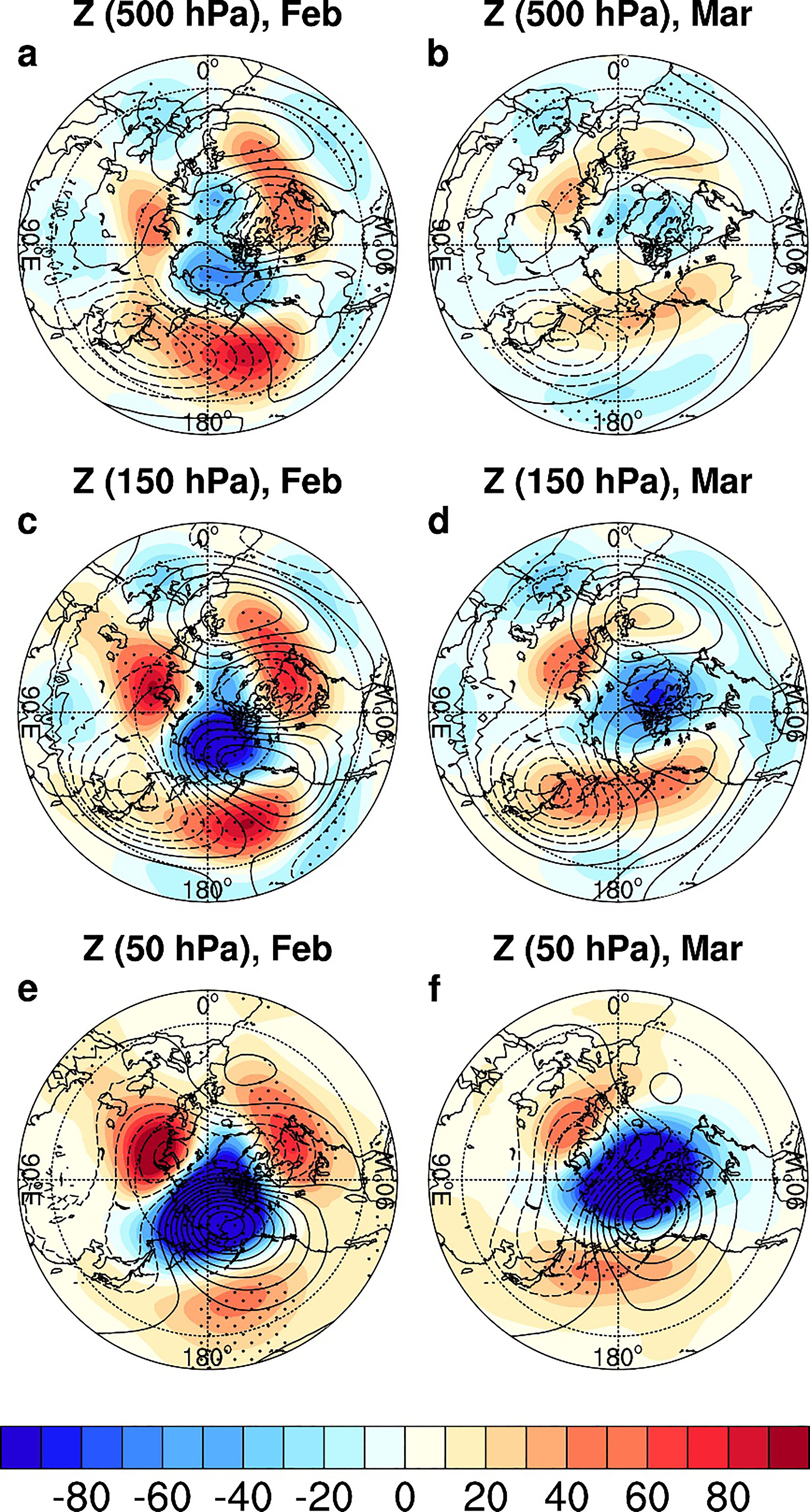 Figure7. Distributions of geopotential height differences between sensitivity and control ensemble simulations (color shading). Upper panels are for 500 hPa in (a) February and (b) March. Middle panels are for 150 hPa in (c) February and (d) March. Lower panels are for 50 hPa in (e) February and (f) March. Color interval is 10 m. Contours in all plots denote climatological mean geopotential heights, with the zonal mean removed. Dotted areas are the regions where the responses are significant at the 90% confidence level (student’s t-test).
Figure 8 shows the wavenumber-1 and wavenumber-2 components of geopotential height differences between sensitivity and control simulations. It is found that the wavenumber-1 wave is weakened, and that the wavenumber-2 wave is enhanced. This is consistent with the observations in Fig. 6. Similarly, ensemble simulations largely underestimate the responses of the planetary waves to SST anomalies.
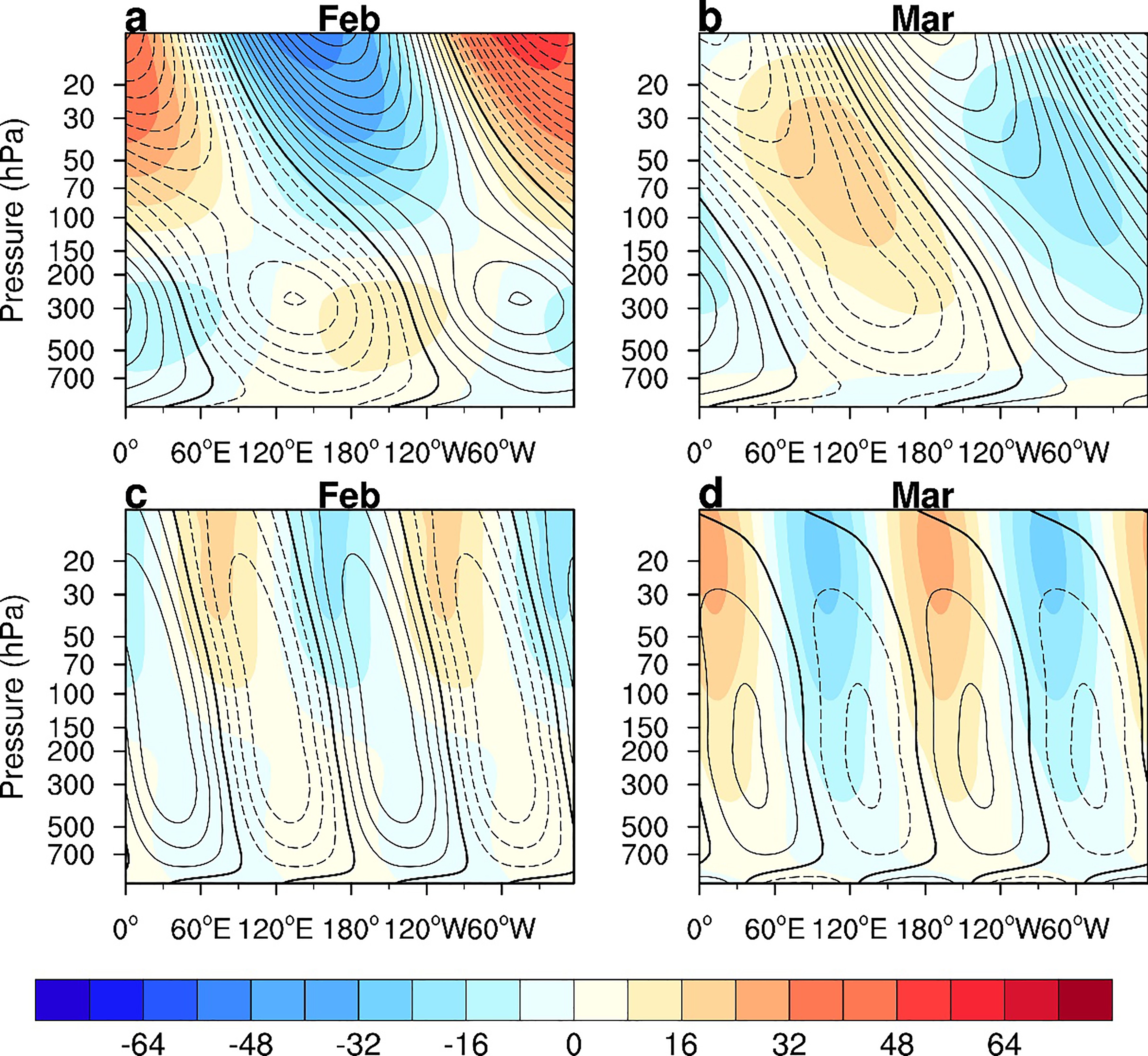 Figure8. Longitude-height sections of geopotential heights decomposed into wavenumber-1 and wavenumber-2 components averaged between 30°N and 70°N in February and March. Upper panels: (a–b) wavenumber-1, and lower panels: (c–d) wavenumber-2. Contours denote the decomposition of the ensemble mean geopotential heights in control simulations, and color shading denotes the differences of the decomposition of geopotential heights between sensitivity and control simulations. The color interval is 8 m.
Figure 9 shows the responses of 50 hPa polar temperatures and total column ozone to warm SST anomalies in the North Pacific. The maximum polar cooling is about 5 K in February and March (Figs. 9a and b). As mentioned above, the cooling amplitude generated by ensemble simulations is much weaker than observations (about 18 K and 24 K in February and March, respectively). Associated with the polar cooling, total column ozone is decreased in the Arctic stratospheric vortex (Figs. 9c and d). The maximum ozone depletion with respect to the ensemble mean in control simulations in March is about 41.2 DU. Similarly, Arctic ozone loss in the ensemble simulations is much weaker than observations because of the large internal variability in ensemble simulations.
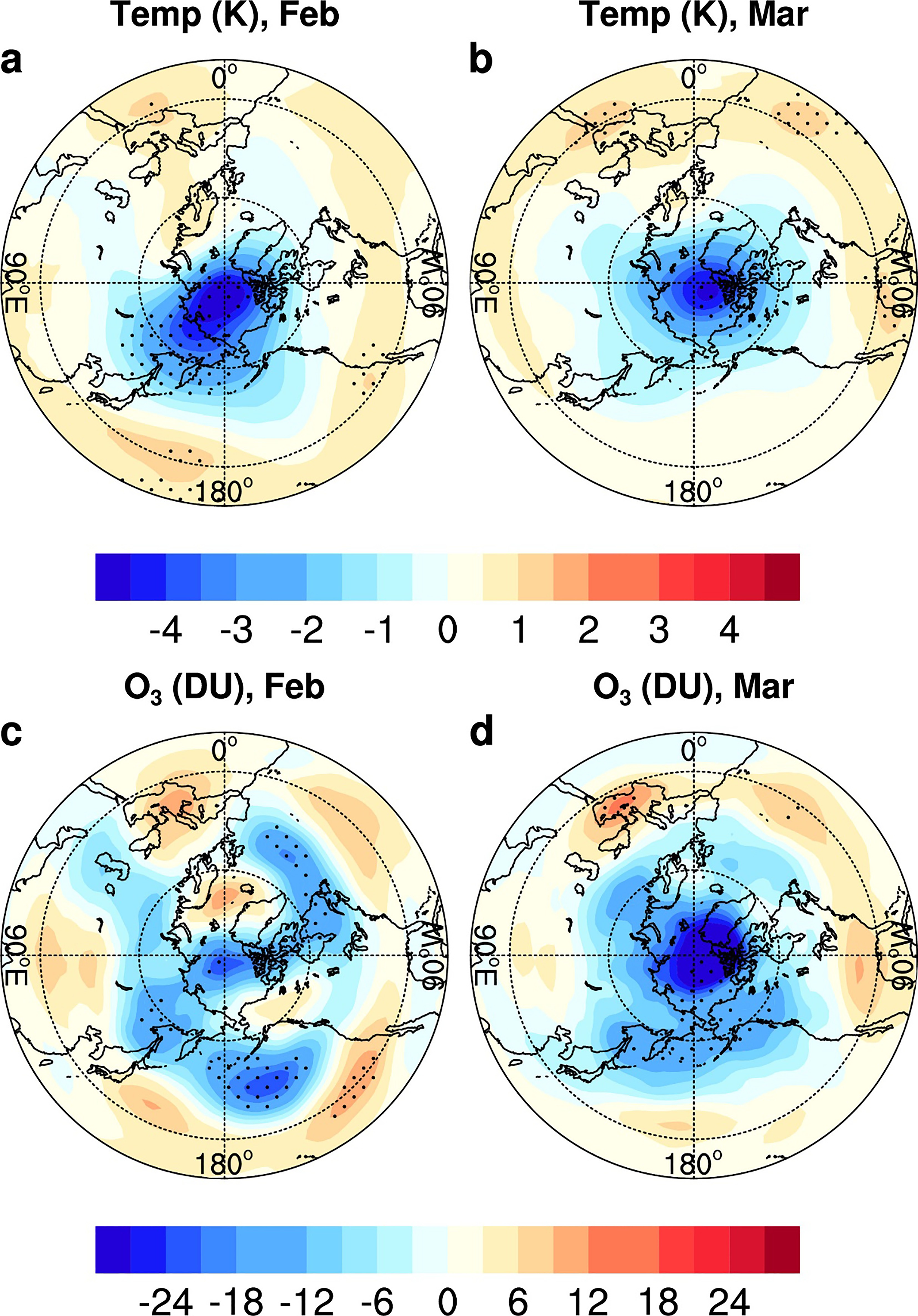 Figure9. Distributions of responses of (a and b) temperatures at 50 hPa and (c and d) total column ozone to warm SST anomalies in the North Pacific in February and March in ensemble simulations. In plots (a) and (b), the color interval is 0.5°C. In plots (c) and (d), the color interval is 3 DU. In all the plots, dotted areas are the regions where the responses are significant at the 90% confidence level (student’s t-test).
Figure 10 shows the probability distribution functions (PDFs) of the daily mean polar temperatures at 50 hPa and total column ozone in March in the sensitivity (blue curve) and control (black) simulations. The probability peak of polar-mean temperatures shifts from about 212 K in the control simulations to about 208 K in the sensitivity simulations (Fig. 10a). The probability peak of polar minimum temperatures shifts from about 198 K to about 189 K (Fig. 10b). The probability peak of polar-mean total column ozone decreases by more than 10 DU (Fig. 10c), which is consistent with the changes of the PDF of the polar mean temperatures. There are two peaks for the PDF of polar minimum ozone. The left peak corresponds to about 260 DU, which is about 80 DU lower than that in the control simulations. Although the ensemble means in polar temperatures and polar total column ozone are weaker than observations, the simulations indicate that warm SST anomalies in the North Pacific are indeed able to cause a colder Arctic stratospheric polar vortex and lower Arctic total column ozone by weakening wavenumber-1 wave amplitude.
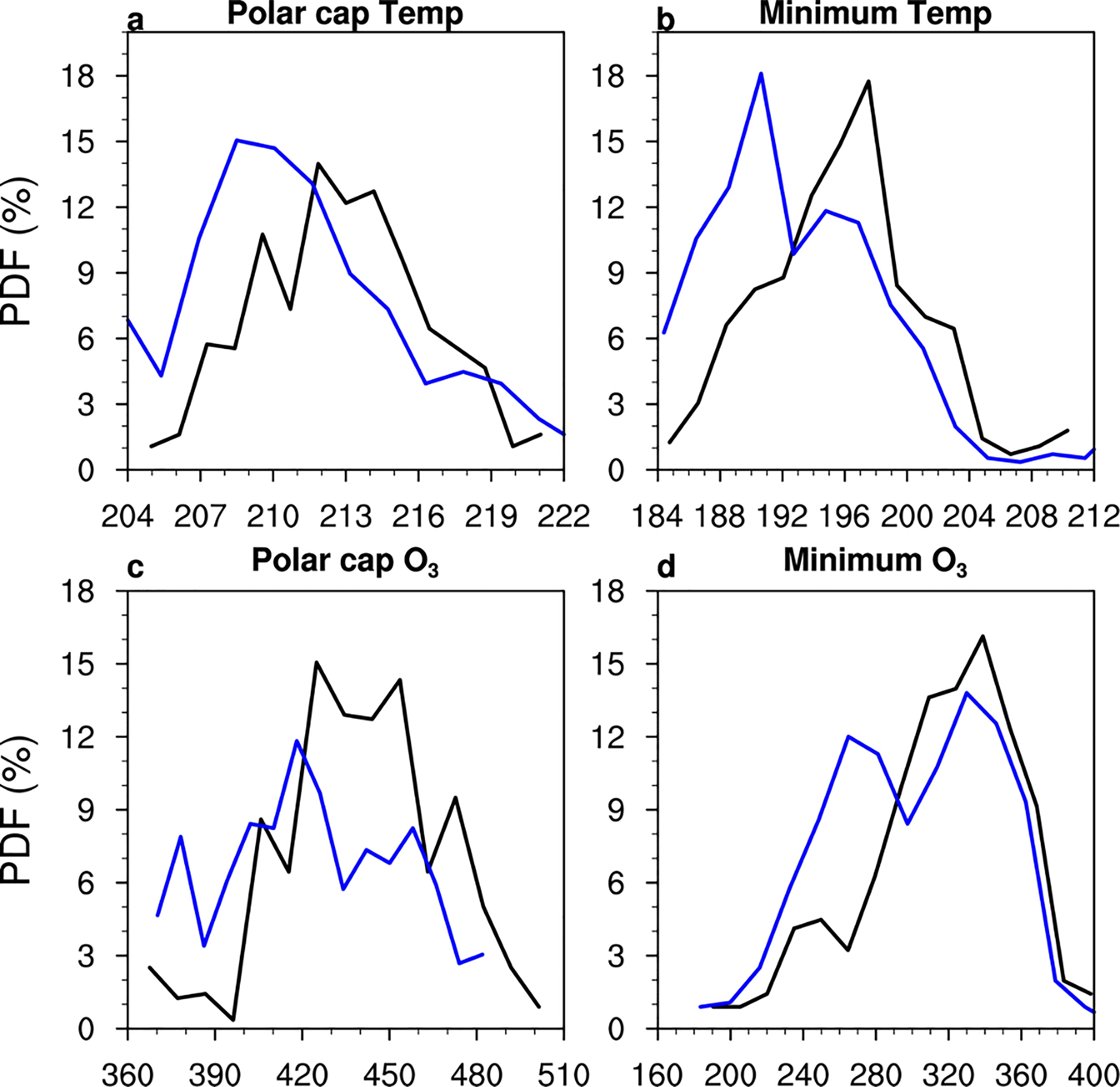 Figure10. Probability distribution functions (PDFs) of daily polar temperatures at 50 hPa and polar total column ozone in March in sensitivity and control simulations. Upper panels: (a) polar-mean temperatures area-weighted over 60°–90°N, and (b) polar minimum temperatures. Lower panels: (c) polar-mean total column ozone area-weighted over 60°–90°N, and (d) polar minimum total column ozone. In all plots, black and blue curves denote the PDFs for control and sensitivity experiments, respectively. The PDFs are calculated using daily mean output from 20 ensemble numbers of sensitivity and control experiments.
Our ensemble simulations further verify that warm SST anomalies in the North Pacific in January–March of 2020 caused a colder Arctic stratospheric vortex and enhanced ozone depletion. Similar to the observational results, simulations forced with North Pacific warm SST anomalies generate weakened amplitudes of wavenumber-1 wave, a colder Arctic stratospheric vortex, and a reduction of total column ozone in the Arctic, although the responses to North Pacific warm SSTs in the ensemble simulations are much weaker than observations. Thus, both the observational analysis and modelling results suggest that severe Arctic ozone loss in spring 2020 was likely caused by the record-high SSTs in the North Pacific. Similarly, the severe ozone depletion in spring 2011 may also be associated with warm SST anomalies in the North Pacific (Hurwitz et al., 2011, 2012). At the current stage, it is not clear whether the record-high SSTs in the North Pacific are an event of natural variabilities or a result of global greenhouse warming.
The formation of the record Arctic ozone loss in spring 2020 indicates that present-day ozone depleting substances are still sufficient to cause severe springtime ozone depletion in the Arctic stratosphere. The above results suggest that severe ozone loss is likely to occur in the near future as long as North Pacific warm SST anomalies or other dynamical processes are sufficiently strong.
Acknowledgements. We thank Dr. Jian YUE for helpful comments. This work is supported by the National Natural Science Foundation of China (NSFC) under Grant No. 41888101. Y. XIA is supported by the Second Tibetan Plateau Scientific Expedition and Research Program (STEP), Grant No. 2019QZKK0604, Key Laboratory of Middle Atmosphere and Global Environment Observation (LAGEO-2020-09), and the Fundamental Research Funds for the Central Universities. The authors declare that datasets for this research are available in the following online repository. The satellite observations of the total column ozone can be found at
