Yuanyuan QIAN^1,2,
Yuhan LUO^1,,,
Fuqi SI¹,
Taiping YANG¹,
Dongshang YANG¹

Corresponding author: Yuhan LUO,yhluo@aiofm.ac.cn;

1.Key Laboratory of Environmental Optical and Technology, Anhui Institute of Optics and Fine Mechanics, Hefei Institutes of Physical Science, Chinese Academy of Sciences, Hefei 230031, China
2.University of Science and Technology of China, Hefei 230026, China
Manuscript received: 2020-07-21
Manuscript revised: 2020-12-29
Manuscript accepted: 2021-01-12
Abstract:Ozone vertical column densities (VCDs) were retrieved by Zenith Scattered Light-Differential Optical Absorption Spectroscopy (ZSL-DOAS) from January 2017 to February 2020 over Fildes Peninsula, West Antarctica (62.22°S, 58.96°W). Each year, ozone VCDs started to decline around July with a comparable gradient around 1.4 Dobson Units (DU) per day, then dropped to their lowest levels in September and October, when ozone holes appeared (less than 220 DU). Daily mean values of retrieved ozone VCDs were compared with Ozone Monitoring Instrument (OMI) and Global Ozone Monitoring Experiment 2 (GOME-2) satellite observations and the Modern-Era Retrospective analysis for Research and Applications Version 2 (MERRA-2) reanalysis dataset, with correlation coefficients (R²) of 0.86, 0.94, and 0.90, respectively. To better understand the causes of ozone depletion, the retrieved ozone VCDs, temperature, and potential vorticity (PV) at certain altitudes were analyzed. The profiles of ozone and PV were positively correlated during their fluctuations, which indicates that the polar vortex has a strong influence on stratospheric ozone depletion during Antarctic spring. Located at the edge of polar vortex, the observed data will provide a basis for further analysis and prediction of the inter-annual variations of stratospheric ozone in the future.
Keywords: ozone VCDs,
ZSL-DOAS,
Antarctic ozone depletion,
polar vortex
摘要:利用天顶散射光差分吸收光谱技术（ZSL-DOAS），观测了2017年1月至2020年2月西南极菲尔德斯半岛（62.22°S, 58.96°W）上空的臭氧垂直柱浓度（VCD）。结果显示，臭氧VCD在每年的7月以每天1.4 DU的梯度下降，在9-10月下降至最低水平，并出现臭氧空洞（臭氧VCD小于220 DU）。将地基反演的臭氧VCD每日均值与OMI、GOME-2卫星观测结果和MERRA-2再分析数据进行对比，相关性（R²）分别为0.86、0.94与0.90。为了进一步探究臭氧损耗成因，对臭氧VCD、温度与位涡（PV）进行了分析。结果显示，在臭氧波动期间，臭氧与PV的垂直廓线呈现正相关趋势，这表明在南极春季极涡对平流层臭氧的损耗有关键的影响。由于观测站点位于极涡边界区域，该站点的持续观测数据将为臭氧损耗的进一步分析和平流层臭氧的年际变化预测提供依据。
关键词:臭氧垂直柱浓度,
天顶散射光差分吸收光谱技术,
南极臭氧损耗,
极涡

HTML

--> --> -->

Ozone is an important trace gas in the Earth’s atmosphere that impacts the environment, climate change, and human health (Li et al., 2015). It is most prevalent about 20?35 km above the surface of the Earth, where it can absorb UV radiation to protect life on Earth. The ozone hole was first discovered by Farman in Argentine Islands (65°S, 64°W) and Halley Bay (76°S, 27°W), Antarctica (Farman et al., 1985). Long-term trends in ozone column measurements, obtained from South Pole stations and Solar Backscatter Ultra Violet (SBUV) satellite observations, indicate that healing of Antarctic ozone holes is occurring based on control of Hydrochlorofluorocarbons emissions (Solomon et al., 2016).
Accurate retrieval of ozone columns, as well as comprehensive analysis of stratospheric chemistry, dynamics and temperature changes on ozone columns is necessary for the analysis of Antarctic ozone changes. Ozone columns over Antarctica are mainly obtained from satellite observations, ground-based DOAS observations, Brewer spectrophotometers, and Dobson spectrophotometers (?í?ková et al., 2019; Kokhanovsky et al., 2020). Satellite observations and European Centre for Medium-Range Weather Forecasts (ECMWF) data were analyzed to study the influence of stratospheric halogen species (mainly Cl and Br) in the polar vortex, which may lead to ozone depletion over Antarctica (Marsing et al., 2019; Nakajima et al., 2020). In addition, an atmospheric and chemical transport model is used for the analysis of long-term ozone trends and troposphere-stratosphere exchange in Antarctica (Hegglin and Shepherd, 2009; Lu et al., 2019).
The atmosphere over Antarctica is controlled by the strong polar vortex in winter, making it difficult to exchange with mid-latitude atmosphere. The extremely low air temperatures (< ?78°C) inside the polar vortex, lead to the formation of polar stratospheric clouds (PSCs). PSCs, composed of nitrate trihydrate, water ice, etc., provide surfaces for heterogeneous reactions that convert halogen reservoirs to active halogens causing severe ozone depletion (Frieβ et al., 2005; Drdla and Müller, 2012; Marsing et al., 2019). There are three types of PSCs (decided by their state), including nitric acid trihydrate (NAT), supercooled ternary solution (STS), and ice PSCs, and their corresponding temperatures are $ {T}_{\rm{nat}} $ (?78°C), $ {T}_{\rm{sts}} $, and $ {T}_{\rm{ice}} $. The observation site is located at the edge of the polar vortex, which is different from other inland stations (high latitudes) where the ozone columns continued to be low in spring. The rapid changes and great fluctuations of total ozone can be detected at the observation site location and are sensitive to the dynamic and chemical changes of PSCs.
As a spectroscopic technique, differential optical absorption spectroscopy (DOAS) has been proven to be powerful and has been widely used to monitor a variety of atmospheric trace gases (Stutz and Platt, 1997; Meller and Moortgat, 2000; Platt and Stutz, 2008). Zenith Scattered Light-DOAS (ZSL-DOAS) is suitable for measuring stratospheric gases, such as stratospheric $ {\rm{NO}}_{2} $ and $ {\rm{O}}_{3} $ (Pommereau, 1982; Perner et al., 1994). Since the 1970s, numerous spaceborne UV detection instruments (such as Ozone Monitoring Instrument (OMI), Global Ozone Monitoring Experiment 2 (GOME-2), and Microwave Limb Sounder (MLS)) have been launched to observe global trace gases, and their observations have provided comprehensive information on ozone holes and changes (Sonkaew et al., 2013; Zhang et al., 2015; Kuttippurath and Nair, 2017). Some advantages of ZSL-DOAS are that it has low energy consumption and can be unattended, and it is less affected than satellite-based instruments by changes of meteorological conditions in the boundary layer, temperature, and clouds.
In this study, daily variations of ozone vertical column densities (VCDs) are retrieved by ZSL-DOAS, and a correlation analysis is performed between the ZSL-DOAS measurements and OMI, GOME-2 observations and Modern-Era Retrospective analysis for Research and Applications version 2 (MERRA-2). Combining observed ozone VCDs and low-stratospheric PV profiles, the cause of ozone depletion leading to ozone holes from September to October in 2017 and 2018 in the experiment region (62.22°S, 58.96°W) at the edge of the polar vortex is investigated. The aim of this study is to analyze the correlation between ozone depletion and PV at the edge of the polar vortex, where ozone depletion is more sensitive to changes in PV.

2

-->

2.1. Experiment site

The experiment site and DOAS instrument are shown in Fig. 1. The red star is the location of Chinese Great Wall Station (62.22°S, 58.96°W) in Fildes Peninsula, South Shetland Islands. The red region is the area of the OMI pixel, and the yellow region is the area of the GOME-2 pixel.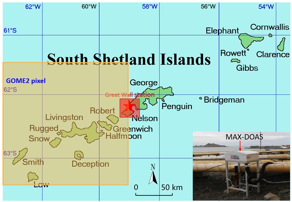
Figure1. Instrument and experiment site (red star) and pixels of OMI and GOME-2 observations (red and yellow boxes).


The ground-based passive DOAS system used in this experiment is composed of key parts such as a prism, telescope, motor, filter, CCD spectrometer, and computer. The wavelength range of the spectrometer is 290?420 nm, and the spectral resolution is 0.3 nm. In this experiment, the data from zenith direction is used to retrieve the slant column densities (SCDs) of ozone.

2 -->

2.2. Principles of the DOAS method

The DOAS method retrieves concentrations of trace gases based on their characteristic absorption and the measured intensity, which is based on Lambert-Beer’s law. From Lambert-Beer’s law and derivation:
here, $ {I}_{0}\left(\lambda \right) $ denotes the original luminous intensity of the radiator, $ {I}^{*}\left(\lambda \right) $ represents the measured intensity after filtering through a gas layer of length L, $ {\sigma }_{j}^{*}\left(\lambda \right) $ denotes the broadband absorption cross section at the wavelength $ \lambda $, $ {c}_{j} $ represents the average concentration of gas j, ${\rm{SC}}{{\rm{D}}_j} = \int {{c_j}L} $ is the slant column density of j, and $D = \ln [{{{I^ * }\left(\lambda \right)}}/{{{I_0}\left(\lambda \right)}}]$ is the named differential optical density. The SCD of the desired trace gas can be retrieved through least-squares fitting by Eq. (1).

2 -->

2.3. Spectral retrieval

The ozone SCDs are retrieved from the QDOAS software developed by the Royal Belgian Institute for Space Aeronomy (BIRA-IASB) (http://uv-vis.aeronomie.be/software/QDOAS/), with a retrieval wavelength range of 320?340 nm. $ {\rm{O}}_{3} $, $ {\rm{NO}}_{2} $, $ {\rm{O}}_{4} $, and ring (the rotational Raman scattering effect, calculated by Ring.exe of QDOAS) cross sections are considered in the retrieval algorithm, and detailed parameters are shown in Table 1. The daily noon zenith spectrum is used as the reference spectrum for SCD retrieval. Taking the fits of the spectrum from 24 February 2018 as an example (Fig. 2), the differential slant column density (dSCD) of ozone is $ 5.20\times {10}^{18} $ molec cm^?2, with the root mean square (RMS) of spectral fitting residual of 9.76×10^?4.

Parameter	References
$ {\rm{O}}_{3} $	223 K, 243 K (Bogumil et al., 2003)
$ {\rm{NO}}_{2} $	298 K (VanDaele et al., 1996)
$ {\rm{O}}_{4} $	293 K (Hermans et al., 2003)
Ring	Ring.exe
Fitting Interval	320?340 nm
Polynomial	5

Table1. Fitting parameters of spectral retrieval.


Figure2. Spectrum fits of ozone on 24 February 2018.



2 -->

2.4. Calculation of ozone VCDs

The ZSL-DOAS method is powerful in measuring stratospheric gases such as ozone. To convert SCD (related to the viewing angles) into vertical column density (VCD), the Air Mass Factor (AMF) must be introduced. The relationship between SCD and VCD is as follows:
AMFs are retrieved from the atmospheric radiative transfer model SCIATRAN. The a-priori profiles of ozone, temperature, and pressure used to obtain AMFs are the monthly average profiles from the SCIATRAN profiles database, which are selected by month and latitude. The Fraunhofer absorption, which will have a strong influence on the retrieval of gas concentration, should be removed (Platt and Stutz, 2008). The slant column concentration after deducting Fraunhofer absorption is expressed by the dSCD:
Here, $ {\rm{SCD}}_{\rm{FRS}} $ refers to the Fraunhofer absorption part. The above formula is in y=ax+b format, so we can use AMF as the abscissa and dSCD as the ordinate to perform linear fitting, where the slope is VCD and the absolute value of the intercept is the Fraunhofer absorption part. Taking the retrieved data from 24 February 2018 as an example, the linear fit of ozone dSCDs and AMFs on that day is shown in Fig. 3. The calculated ozone VCD is $ 7.322\times {10}^{18} $ molec cm^?2 and the error is $ 2.232\times {10}^{16} $ molec cm^?2. The ozone VCD is calculated by the average of VCD_am (the VCD of morning) and VCD_pm (the VCD of afternoon).
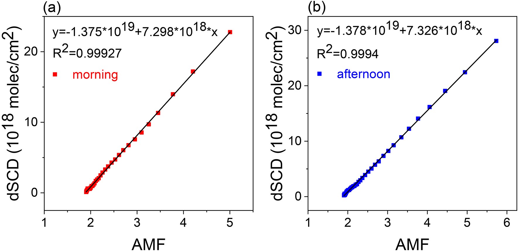Figure3. Linear fitting between ozone dSCDs and AMFs for morning (a) and afternoon (b) on 24 February 2018. The correlation coefficients (R²) are 0.99927 and 0.9994. The ozone VCDs for morning and afternoon are 7.298 × 10¹⁸ molec cm^?2 and 7.326 × 10¹⁸ molec cm^?2. The calculated ozone VCD for 24 February 2018 is 7.322 × 10¹⁸ molec cm^?2.


The uncertainty of ozone VCD retrieval through the ZSL-DOAS method comes from the retrieval of SCD and AMF. The comprehensive estimation of uncertainty of ozone SCDs is 1.475% (95% confidence interval, N = 76 902). Parameters including SZA (solar zenith angle), surface albedo, a-priori ozone profile, and wavelength, which would influence the values of AMF, are considered. In this study, the SZA used for calculation is between 35° and 80°, and the surface albedo is between 0.08 and 0.6. The a-priori profile of ozone is obtained from the monthly mean climatology. The detailed parameter nodes to estimate the uncertainty of AMF on wavelength are shown in Table 2. The AMF uncertainty caused by wavelength selection is calculated through $ \left({\rm{AMF}}_{\lambda }-{\rm{AMF}}_{328}\right)/{\rm{AMF}}_{\lambda } $, where $ \lambda $ denotes wavelength. In the simulated parameter nodes (Table 2), the AMF uncertainty on wavelength is between ?4.257% and 4.630%, with the averaged absolute uncertainty being 2.030%. According to the analysis of the OMI ozone product, the variations of AMF influenced by a-priori profiles of ozone are small (2% on the 95% confidence interval) (Bhartia, 2002). Therefore, the averaged AMF uncertainty with this method is calculated through $\sqrt {{\rm{AMF}}_{{\rm{uncertainty}}\_{\rm{wave}}}^2 + {\rm{AMF}}_{{\rm{profile}}}^2} $, and is 2.85%. The total uncertainty of VCD is 3.21%, based on the error propagation formula as follows:

Parameters	Nodes
SZA	35°, 40°, 45°, 50°, 55°, 60°, 65°, 70°, 75°, 80°
Surface albedo	0.05, 0.1, 0.2, 0.3, 0.4, 0.5, 0.6
Wavelength	From 320 to 340 nm in 0.5 nm interval

Table2. Parameter nodes to estimate the AMF uncertainty on wavelength.



2 -->

2.5. Auxiliary data

The daily ozone VCDs observed by OMI and GOME-2 from January 2017 to February 2020 are obtained for this study. The OMI, launched on 15 July 2004, is onboard the Aura satellite and is a nadir scanning instrument (Xie et al., 2016). The field of view of the OMI can reach 114°, which permits daily global coverage. The OMI can measure ozone in UV (270?380 nm) and VIS (350?500 nm) wavelengths. The spectral resolution of the OMI is 0.5 nm, with high spatial resolution of $ 13\times 24\;{\rm{km}}^{2} $ (Thomas et al., 2011). The daily ozone VCDs from the OMI (https://disc.gsfc.nasa.gov/) are used to compare with ZSL-DOAS observations.
GOME-2 is a UV/VIS nadir observation spectrometer, which is onboard the MetOp-A satellite and was launched on 19 October 2006 by the European Space Agency (ESA). The ozone data sets of GOME-2 are retrieved by the GOME-type Direct FITting (GODFIT) v4 algorithm. The wavelength range of the GOME-2 instrument is 240?790 nm. The spectral resolution of GOME-2 is 0.2?0.5 nm, with spatial resolution of $ 80\times 40\;{\rm{km}}^{2} $ (Koukouli et al., 2014). The ozone VCDs obtained from the GOME-2 data set (https://avdc.gsfc.nasa.gov/) are daily mean VCDs of the overpass data.
The temperature and ozone profiles used here are obtained from MERRA-2 data and are available every 3 hours. MERRA-2 is an atmospheric reanalysis database, obtained from Goddard Earth Observing System Model, version 5 (GEOS-5) with Atmospheric Data Assimilation System (ADAS) (Ganeshan and Yang, 2019). The spatial resolution of MERRA-2 is ${0.5^\circ } \times {0.625^\circ }\;\left({{\rm{lat}} \times {\rm{lon}}} \right)$ with 72 model levels. The ozone profiles and temperature at 50 hPa from MERRA-2 (https://disc.gsfc.nasa.gov/) are daily averages.
The daily PV data used in this study is obtained from ERA Interim datasets from the ECMWF website (https://www.ecmwf.int/). ERA Interim is a 6-hourly reanalysis dataset, which is available from January 1985 to August 2019. The ERA Interim datasets are obtained from the data assimilation system of the Integrated Forecast System (IFS), released in 2006. The spatial resolution of ERA Interim data is ${0.25^\circ } \times {0.25^\circ }\;\left({{\rm{lat}} \times {\rm{lon}}} \right)$, with 60 levels in the vertical direction from the surface to 0.1 hPa.

2

-->

3.1. Meteorological conditions

The meteorological conditions of the Fildes Peninsula are shown in Figs. 4 and 5, which represent temperatures (at 50 hPa) and PV (on isentropic level of 475 K) respectively. $ {T}_{\rm{nat}} $ denotes the threshold temperature for the formation of PSCs. The temperature trends during the experimental period show that the formation of PSCs began around June, which corresponds to the development of the polar vortex in early winter (Frieβ et al., 2005). Additionally, the overall temperature of 2019 was higher than 2018 and 2017 and had an early termination of low temperatures, which led to the short existence of PSCs.
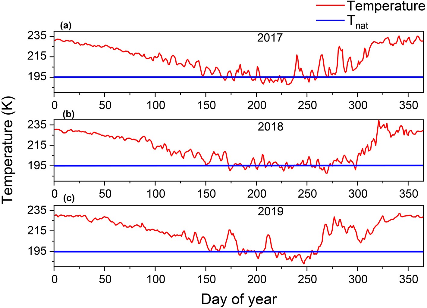Figure4. Temperatures (at 50 hPa) over Fildes Peninsula from 2017 to 2019, where the blue lines denote the threshold temperature for the formation of PSCs.


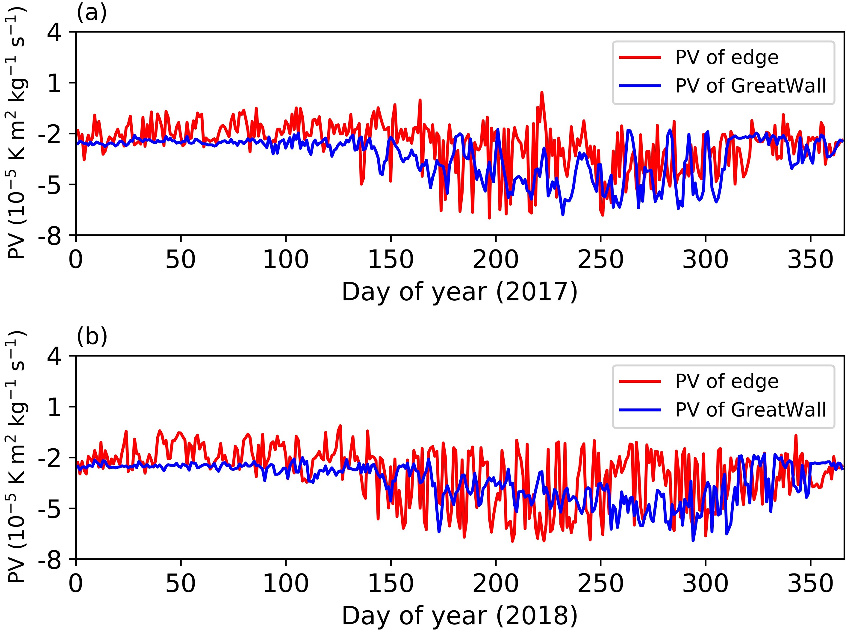Figure5. PV (on isentropic level of 475 K) of the Fildes Peninsula and vortex edge, where red and blue lines denote PV of vortex edge (calculated by Nash’s criterion) and Fildes Peninsula, respectively. (a) The PV in 2017. (b) The PV in 2018.


PV is used to represent the capacity for an air mass to rotate in the atmosphere and to define the edge of the polar vortex. PV is calculated using other parameters such as temperature, wind field, etc. The units of PV (potential vorticity units, PVU) are a combination of SI units (${\rm{K}}\;{{\rm{m}}^2}\;{\rm{k}}{{\rm{g}}^{ - 1}}\;{{\rm{s}}^{ - 1}}$), where $1\;{\rm{PVU}} = {10^{ - 6}}\;{\rm{K}}\;{{\rm{m}}^2}\;{\rm{k}}{{\rm{g}}^{ - 1}}\;{{\rm{s}}^{ - 1}}$. In Fig. 5, the 475 K potential temperature surface, which corresponds to the lower stratosphere, is used as the criterion to define the edge of polar vortex (Paschou et al., 2020), and blue lines denote the PV of the Fildes Peninsula and red lines denote the PV of the vortex edge. Nash’s criterion, where the gradient of PV is the highest of the southern hemisphere along the equivalent latitude (Nash et al., 1996), is used to determine the edge of the polar vortex. The blue line being below (above) the red line indicates that the Fildes Peninsula is located inside (outside) of the polar vortex. The number of days inside and outside the polar vortex boundary in 2017 and 2018 are shown in Table 3.

Date	Days inside polar vortex	Days outside polar vortex
2017	273	92
2018	235	130
2017.9?10	39	22
2018.9?10	45	16

Table3. The number of days inside and outside the polar vortex.



2 -->

3.2. Results of ozone VCDs

Satellite ozone observations may have large biases at high latitudes, especially when the SZAs are large. Therefore, the SZAs used to obtain ozone VCDs from satellite observations are less than 86°. The ZSL-DOAS observations in this study can be used to validate the satellite observations at high latitude.
The ozone VCDs retrieved from the ZSL-DOAS instrument, the MERRA-2 dataset and satellite observations from OMI and GOME-2 from January 2017 to February 2020 are shown in Fig. 6a, where the black line located at 220 DU ($1\;{\rm{DU}} = 2.69 \times {10^{16}}{\rm{molec}}\;{\rm{c}}{{\rm{m}}^{ - 2}}$) denotes the threshold for an ozone hole (Bodeker et al., 2002). The biases between OMI, GOME-2, MERRA-2, and ZSL-DOAS are shown in Fig. 6b. The standard deviations between GOME-2, MERRA-2, and ZSL-DOAS are shown in Fig. 6c. OMI and GOME-2 are nadir observations that are different from the zenith observation method of ZSL-DOAS. The ozone VCDs of satellite observations could only be obtained at overpass times (1330 LST and 0930 LST), which may have led to the large biases and standard deviations when ozone fluctuated greatly on that day.
Figure6. (a) The ozone VCDs from ZSL-DOAS, OMI, GOME-2, and MERRA-2. The black line denotes the threshold for ozone holes. (b) The biases of OMI, GOME-2, and MERRA-2. (c) The standard deviations of GOME-2 and MERRA-2.


The averaged ozone VCDs and ozone hole days for 2017, 2018, and 2019 over the Fildes Peninsula are shown in Table 4. Ozone VCDs start to decline around July with a comparable gradient (around 1.4 DU d^?1), which is in agreement with the formation of PSCs in Antarctic winter. Ozone VCDs decline further in the spring, with severe ozone depletion in September and October, and then gradually return to normal levels. During the severe ozone depletion periods in September and October, which lead to the ozone holes (<220 DU), there is a correlation between the polar vortex and ozone concentration, which is discussed in detail in section 3.3. The linear fits of the retrieved ozone VCDs with OMI and GOME-2 satellite observations and the MERRA-2 dataset are shown in Fig. 7. The correlation coefficients ($ {R}^{2} $) are 0.86, 0.94, and 0.90, respectively.

Date	Average ozone VCDs (DU)	Ozone hole days
2017	295.85	16
2017.9?10	260.76	15
2018	289.32	30
2018.9?10	215.13	25
2019	294.04	29
2019.9?10	283.38	22

Table4. Averaged ozone VCDs and ozone hole days.


Figure7. Scatter plots and linear fit of retrieved ozone VCDs with (a) OMI, (b) GOME-2, and (c) MERRA-2.



2 -->

3.3. Influence of PV on ozone depletion

The sign of PV is negative in Antarctica while positive in the Arctic. The absolute value of PV is generally greater inside the polar vortex. The PSCs formed inside the polar vortex can activate the halogen species, which lead to severe ozone depletion. The PV, temperatures (at 50 hPa), and retrieved ozone VCDs from September to October during the observation period are shown in Fig. 8. As shown in Figs. 8a-d, the trend of PV and ozone VCDs is similar. In other words, PV is positively correlated with the ozone VCDs. The ozone VCDs fluctuate between 170?405 DU from September to October of 2017. The fluctuations in 2018 are between 150?290 DU. The relationship between PV and ozone VCDs is more obvious in 2017 with greater fluctuations. As shown in Fig. 8a, ozone recovers to its peak values on 22 September, 9 October, 19 October, and 28 October 2017, when Fildes Peninsula is fully outside of the polar vortex. The retrieved ozone VCDs fluctuate with the same pattern as the temperatures at 50 hPa, which means ozone is depleted inside the polar vortex, where the temperature is lower. Therefore, the polar vortex has a strong influence on stratospheric ozone depletion during Antarctic spring.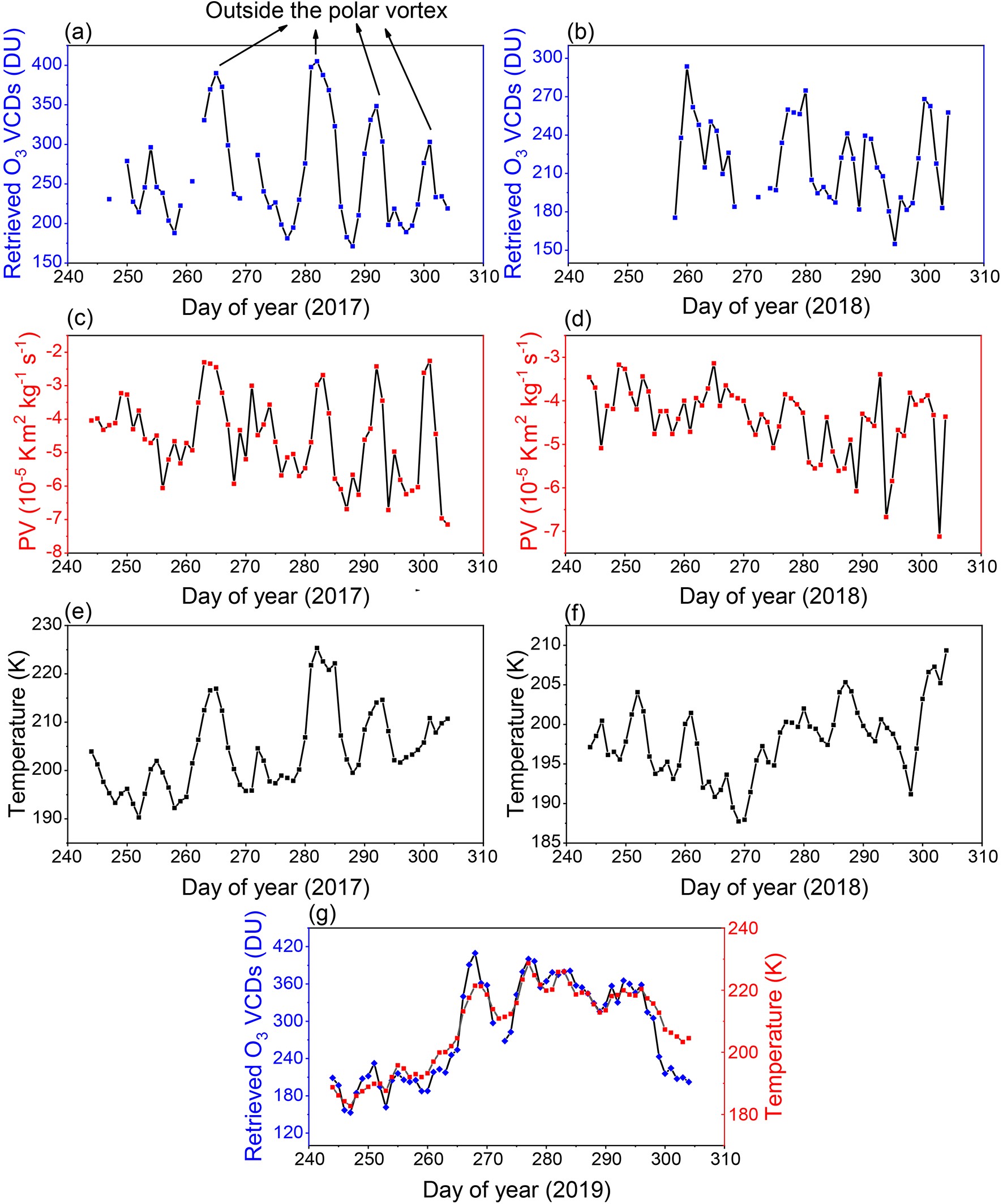
Figure8. Ozone VCDs, PV, and temperatures (at 50 hPa) from September to October during the observation period: (a) retrieved ozone VCDs from September to October in 2017; (b) retrieved ozone VCDs from September to October in 2018; (c) PV (at 50 hPa) from September to October in 2017; (d) PV (at 50 hPa) from September to October in 2018; (e) temperature (at 50 hPa) from September to October in 2017; (f) temperature (at 50 hPa) from September to October in 2018; and (g) retrieved ozone VCDs and temperature (at 50 hPa) from September to October in 2019.


Ozone and PV profiles above the Fildes Peninsula during spring of 2017 and 2018 are analyzed as well. The averaged ozone profiles during the ozone hole periods and non-ozone hole periods from September to October in 2017 are shown in Fig. 9. The averaged ozone profiles and the percentage of ozone loss at different heights indicate that the maximum ozone loss is about 63% at the height of 19.5 km. PV might differ by more than a factor of ten for different heights in the lower stratosphere, which indicates that a small and sensitive height layer should be chosen to discuss its influence on ozone depletion. Therefore, the profile height of 19?20 km, where the photochemical reactions destroying ozone are most severe, was chosen.
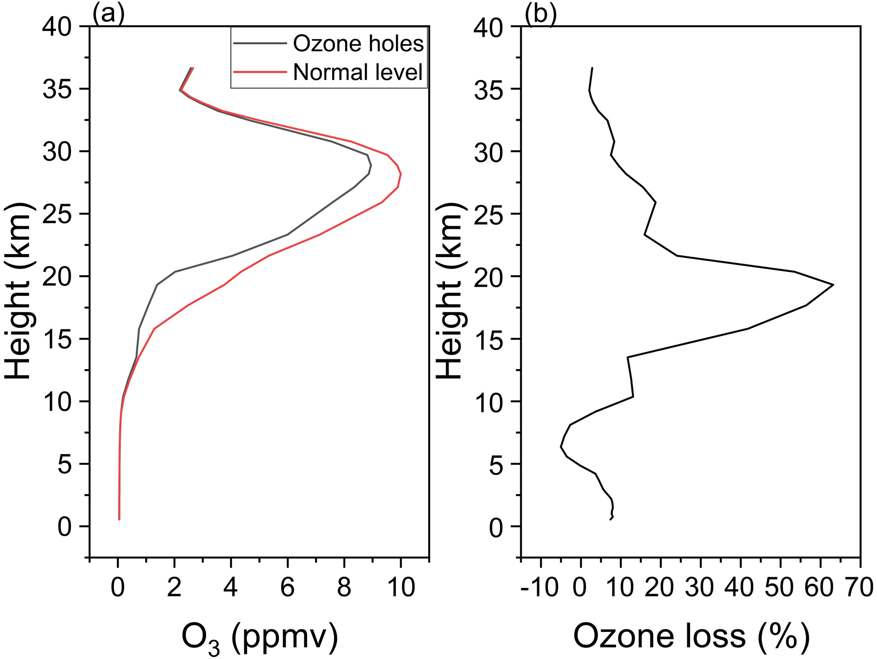Figure9. (a) Averaged ozone profiles during the ozone hole periods and non-ozone hole periods from September to October in 2017. (b) The percentage of ozone loss at different heights calculated by (a).


Since the observation site is located near the edge of the polar vortex, it is sensitive to the changes of the polar vortex. The synchronized change between ozone and PV indicates the critical influence of the polar vortex on ozone depletion. The profiles of ozone and PV at the height of 19?20 km from September to October in 2017 and 2018 are shown in Fig. 10. The ozone concentration at the height of 19?20 km fluctuates between 0.65?6.87 ppmv and 0.54?7.30 ppmv in 2017 and 2018, respectively. The absolute value of PV shows an obvious increase when the ozone concentration decreases. The ozone depletion in Antarctic spring, which leads to the formation of ozone holes, is closely related to PV. Located at the edge of the polar vortex, the observed data will provide a basis for further analysis and prediction of the inter-annual variation of stratospheric ozone in future.
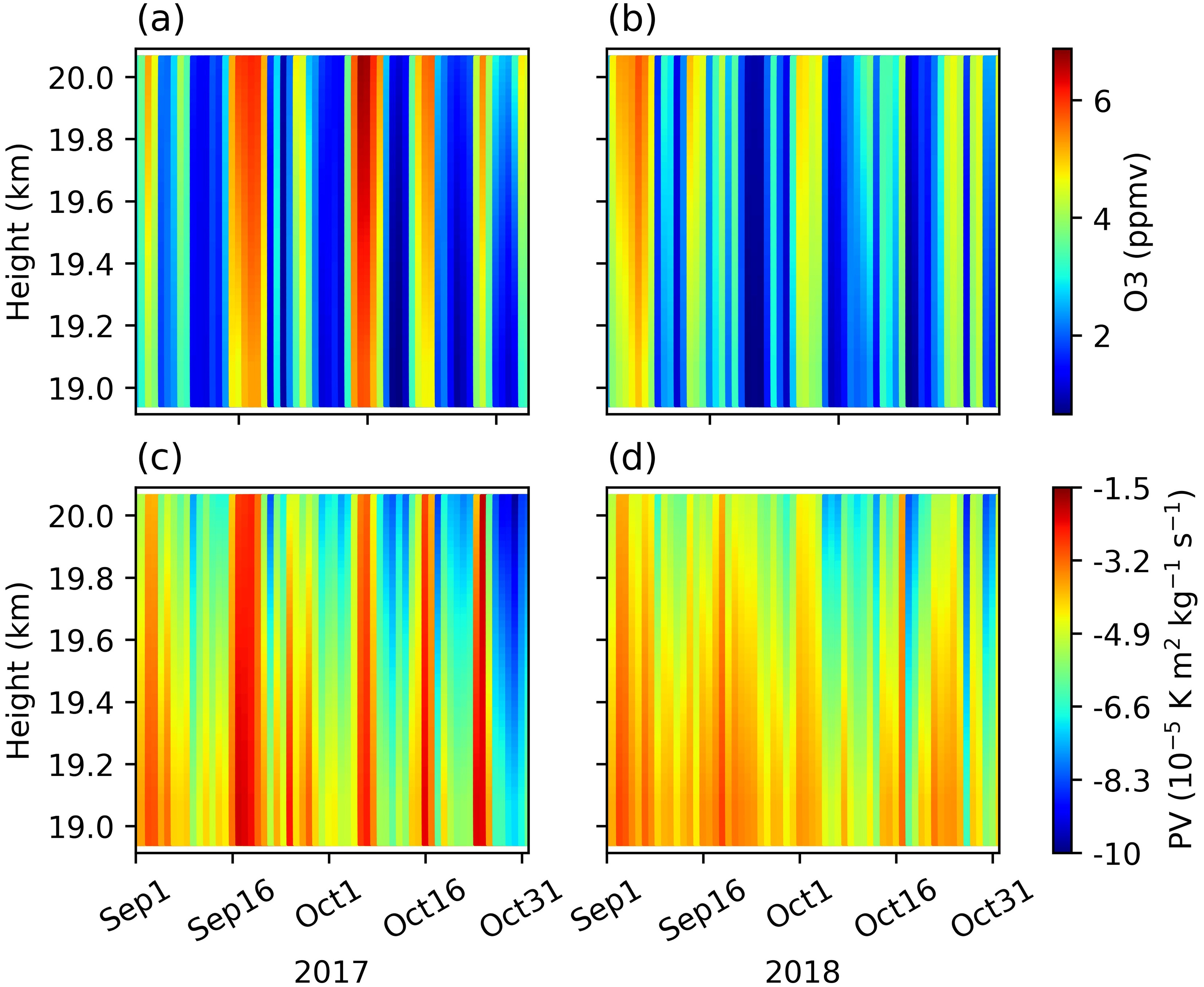Figure10. Profiles of ozone and PV from September to October in 2017 and 2018, at the height of 19?20 km: (a) profile of ozone in 2017; (b) profile of ozone in 2018; (c) profile of PV in 2017; and (d) profile of PV in 2018.

In this study, daily ozone VCDs are retrieved by ZSL-DOAS from ground-based DOAS instrument observations and then linearly fitted with satellite observations from OMI and GOME-2 and reanalysis data from MERRA-2. The correlation coefficients ($ {R}^{2} $) are 0.86, 0.94, and 0.90 respectively, which validate the satellite observations and MERRA-2 dataset for this area.
Each spring during the observation period, occurrences of ozone holes over the Fildes Peninsula were detected when the daily ozone VCDs fluctuated sharply. Especially in September 2017, the daily fluctuations of ozone VCDs reached up to 100 DU. The ozone VCDs began to decrease in early winter with a comparable gradient (1.4 DU d^?1) throughout the observation period, corresponding with the formation of PSCs. The ozone concentration began to recover at the end of October, and returned to normal levels after November.
In this study, PV was used as an indicator for analysis because it was positively correlated with ozone concentration over Fildes Peninsula in spring. The polar vortex of Antarctic spring has a strong influence on stratospheric ozone depletion.
It should be noted that the uncertainty estimation of the AMF calculation is preliminary, and the uncertainty caused by the a-priori ozone profiles needs further analysis. More accurate a-priori ozone profiles (like column-dependent total ozone profiles) and a better reference spectrum (from direct-sun data) will be used in future research.
Observation of ozone VCDs over Fildes Peninsula will be continually conducted to observe the long-term ozone trends in this region. The observations conducted in this study are also valuable for validating modelled ozone concentrations in this region and contribute to better understanding of ozone recovery and stratosphere-troposphere exchange over the polar vortex edge area.
Acknowledgements. This research was financially supported by the National Natural Science Foundation of China (Grant Nos. 41676184 and 41941011). The authors gratefully acknowledge ECMWF (https://www.ecmwf.int/) for providing ERA-Interim reanalysis data and GES-DISC (https://disc.gsfc.nasa.gov/) for providing MERRA-2 data. The authors thank the staff of Great Wall Station for their kind help. The authors acknowledge three anonymous referees for their help on the improvement of the manuscript.