HTML
--> --> -->The contribution of different sources and the spatial distribution of CH4 emissions remain highly uncertain (Kirschke et al., 2013). In the United States, the national CH4 emissions were underestimated by approximately 50% and 70% by the US Environmental Protection Agency (EPA) and the EDGAR inventories, respectively (Miller et al., 2013). The CH4 emissions using a California-specific inventory were underestimated by 37% compared to top-down atmospheric inversions estimated for central California (Zhao et al., 2009). Top-down inverse approaches have also shown that emission inventories are biased low for China (Shen et al., 2014; Huang et al., 2019). However, one study found that the total CH4 emissions estimated using an atmospheric Bayesian inversion were 29% smaller compared to EDGAR estimates in China and attributed the bias to an overestimation of CH4 emissions from rice agriculture during the summer (Thompson et al., 2015). So far, there have been few studies regarding the seasonal variation of CH4 emission sources in China, which severely limits the accuracy of total annual emission estimates. For example, previous studies estimated the CH4 emissions only in cold periods (Hu et al., 2019) when the emissions from rice paddies are expected to be minimal.
It has been argued that bottom-up CH4 emission estimates have greater uncertainty compared to top-down approaches at the regional scale (Dlugokencky et al., 2009, Pison et al., 2018). In contrast to bottom-up approaches, which are driven by process-based models and/or inventories, top-down approaches are driven by concentration observations and coupled to atmospheric transport models. These top-down constraints are essential to reducing process uncertainty in bottom-up flux estimates (Bloom et al., 2016; Saunois et al., 2016; Houweling et al., 2017; Kunik et al., 2019).
The Stochastic Time-Inverted Lagrangian Transport model coupled to the Weather Research and Forecasting model (WRF-STILT) has been used to estimate CO2, CH4, N2O, SO2, and CO emissions (McKain et al., 2012; Kim et al., 2013; Chen et al., 2016; Xi et al., 2016; Hu et al., 2018a). In addition to their application in urban regions, these inverse modeling techniques have also been applied to estimate trace gas emissions associated with natural ecosystems and agricultural regions (Mallia et al., 2015; Xu et al., 2016; Griffis et al., 2017). These applications support that the WRF-STILT model framework is an effective tool for constraining emissions at relatively high temporal and spatial resolution. However, the application of these methods in China remains relatively rare. Recent studies have applied the WRF-STILT model to estimate CO2 and CH4 budgets in the Yangtze River Delta (YRD) region (Hu et al., 2018b, 2019), but these efforts focused only on CH4 emissions during the cold season when there is little interference from natural sources. Natural wetlands are the largest source of CH4 on the global scale (Kirschke et al., 2013). Further, CH4 emissions from water bodies (rivers and lakes) are comparable to emissions from natural wetlands in China (Xu et al., 2014; Xiao et al., 2019). However, CH4 emissions from rice cultivation, natural wetlands, and water bodies remain highly uncertain because they differ in hydrometeorological conditions, carbon substrate availability, and history of human disturbance (Xu et al., 2014; Wei and Wang, 2016).
Urban lands and lands in their vicinity have been identified as CH4 emission hotspots (Wunch et al., 2009). These hotspots are driven by anthropogenic activities related to coal mining, wastewater treatment, rice cultivation, and landfills, which account for 50%–65% of total anthropogenic CH4 emissions (Aydin et al., 2011). Urbanization is occurring at a rapid pace in China. Quantifying CH4 emissions in urbanized regions and understanding drivers of the emissions can help inform local mitigation efforts and sustainable urbanization planning. Further, very little is known about natural CH4 emissions and their relative contribution to China’s total CH4 budget.
Here, we provide a top-down constraint on CH4 emissions in the YRD region, Eastern China, using the WRF-STILT model framework. The model was enabled by near-continuous CH4 concentration observations from a 70-m tall tower in an agricultural-urban domain in Anhui Province. The main objectives were to: 1) Constrain the major CH4 sources within the YRD region at seasonal time scales; 2) Identify the main sources that control the seasonality of CH4 emissions; 3) Assess the relative importance of natural CH4 emissions from wetlands and water bodies in the YRD region; 4) Evaluate if there are important biases in the a priori CH4 emissions associated with the EDGAR bottom-up inventories; and 5) Determine optimal emission scaling factors to estimate the total anthropogenic and natural emissions of CH4 for the YRD region.
2.1. Site and observations
Atmospheric CH4 concentration was measured on a 70-m tall tower in Quanjiao County, Chuzhou, Anhui Province (31.97°N, 118.26°E, 10 m above sea level; Fig. 1). Croplands are the dominant land use type, accounting for 49% of the total area of the YRD. This land use type includes both dryland crops and rice paddies. According to China Statistical Yearbook (National Bureau of Statistics, 2018), rice paddies occupied 15% of the YRD area in 2018. Other land use types include water bodies (6.9%), marshlands (0.22%), forests (32%), impervious surfaces (11%), grasslands (0.94%), shrublands (0.23%), and bare land (0.04%).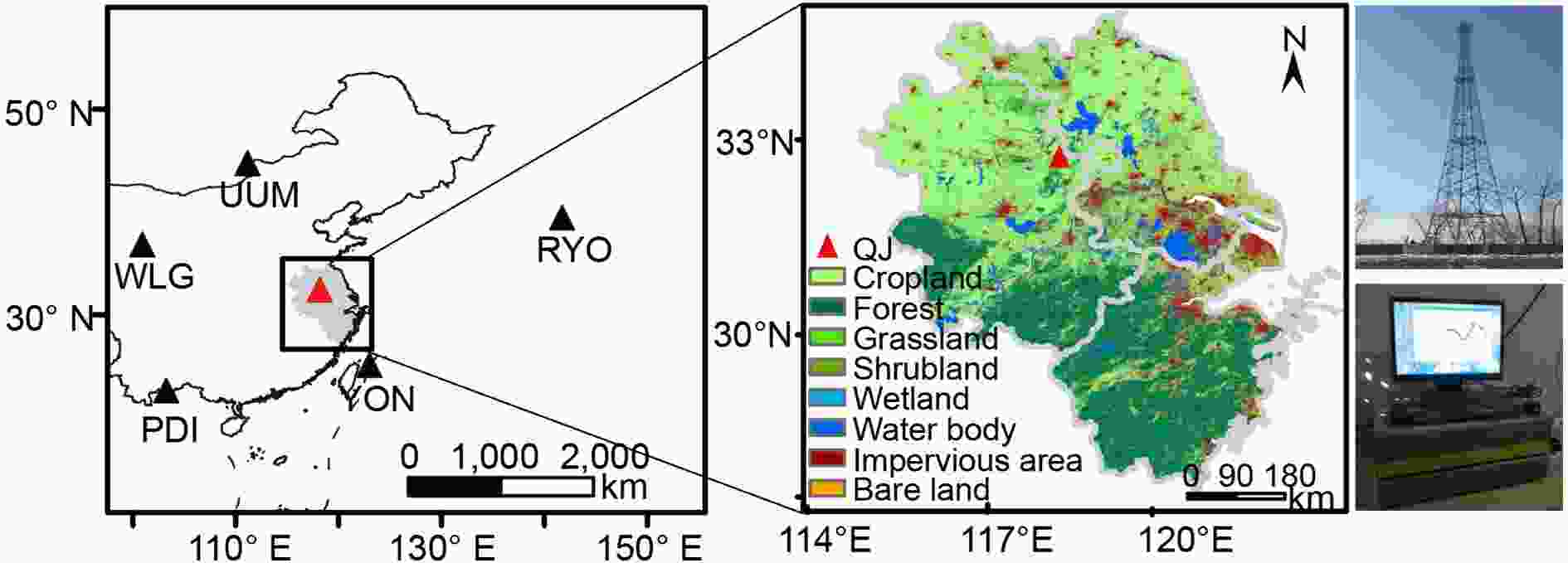 Figure1. Location map and instrumentation. The far-left panel shows the location of the tower site (red triangle) and five WMO/GAW stations, including Ulaan Uul Mongolia (UUM), Waliguang (WLG), Pha Din (PDI), Yonagunijima (YON), and Ryori (RYO). The middle panel is the land cover for YRD at a 30-m spatial resolution (Gong et al., 2019). The two pictures on the far right are the tower and the analyzer.
The tower measurements have been ongoing since December 2017. From December 2017 to December 2018, CH4 concentration was measured using a cavity ring-down spectrometer (model G1301 Picarro Inc., Sunnyvale, CA, USA) at a sampling rate of 1 Hz. In addition to CH4, this instrument also measured CO2 and water vapor concentrations simultaneously. The short-term measurement precision was 0.15 ppm for CO2 and 1 ppb for CH4 based on 5-second averaging internals. The CH4 and CO2 measurements were calibrated twice (24 November 2017 and 10 July 2018). Details about the calibration procedures can be found in the supplemental information.
Supporting measurements included an eddy covariance system consisting of a three-dimensional sonic anemometer (model CSAT3, Campbell Scientific Inc., Logan, UT, USA), an open-path CO2/H2O analyzer (model EC150, Campbell Scientific Inc., Logan, UT, USA), and an air temperature and humidity probe (model HMP155A; Vaisala, Inc., Helsinki, Finland) mounted at the height of 70 m. Additionally, a four-way net radiometer (model CNR4, Kipp & Zonen B. V., Delft, the Netherlands) was mounted at the height of 10 m and provided measurement of upwelling and downwelling of short-wave and long-wave radiation.
2
2.2. WRF-STILT model
We used the Weather Research and Forecasting (WRF) model (version 3.8.1) to provide the meteorological fields (Skamarock et al., 2005; Skamarock and Klemp, 2008) for three nested domains at a spatial resolution of 27, 9, and 3 km (Fig. 2). The innermost domain covers the YRD area. The parameters adopted in WRF have been described by Chen et al. (2016) and Hu et al. (2018a). The initial meteorological fields and boundary conditions were provided by NCEP FNL (Final) Operational Global Analysis data (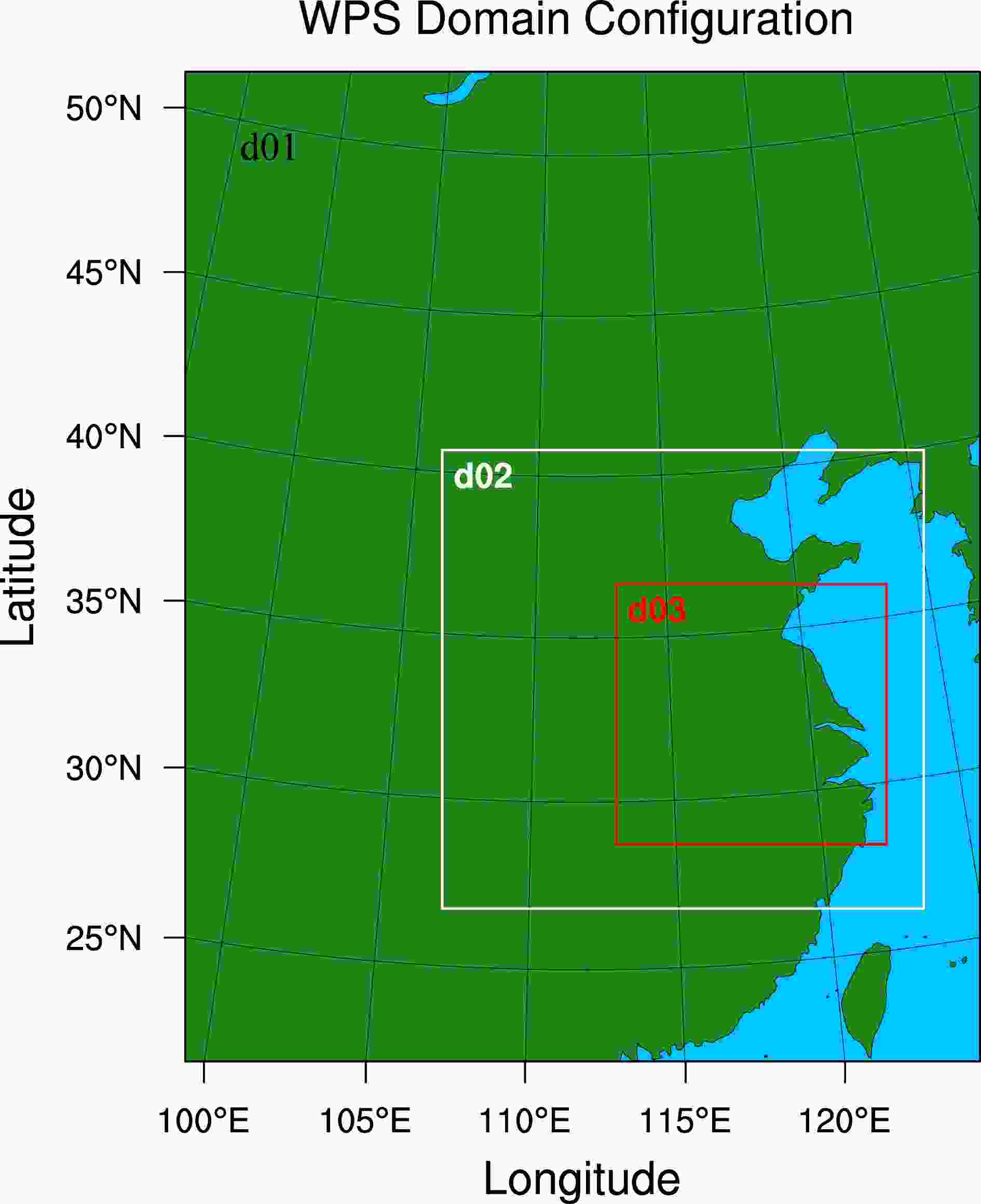 Figure2. WRF configuration of three nested domains. The spatial resolutions for d01, d02, and d03 are 27 km, 9 km, and 3 km, respectively.
The Stochastic Time-Inverted Lagrangian Transport (STILT) model, based on the HYSPLIT model, is a Lagrangian particle dispersion model. A detailed description of the model can be found in Lin et al. (2003). Briefly, the model releases a specified number of particles at the observational location (receptor) and the atmospheric transport, simulated using the WRF model, is used to trace the released particles backward in time. In this way the WRF-STILT model can quantify the contribution from upstream sources or sinks of trace gases to the receptor.
The source/sink contribution, represented by footprint element footprinti,j (units: ppm m2 s μmol?1), is generated from these particle trajectories and their associated locations relative to each grid point. Here, footprinti,j refers to the sensitivity of the CH4 concentration at the receptor with respect to changes in the surface flux at time i and grid j. The use of three domains within WRF provides increased spatial resolution in the innermost domain to reduce uncertainty of the particle trajectory simulation. According to the size of the simulation area (i.e., the outer edge of the domain), the particles are allowed to be transported back in time for up to 168 hours (7 days). Therefore, most of the particles can be traced back to a relatively clean background atmosphere. In the process of atmospheric transport, the particles are affected by the underlying sources and sinks associated with each grid cell, thus producing an enhancement [(ΔCH4)enhancement] on the observed concentration at the receptor. Theoretically, the observed concentration is the sum of the enhancement attributed to these sources and the background concentration (Lin et al., 2003; Mallia et al., 2015; Hu et al., 2019), as expressed by the following equation:
2
2.3. A priori CH4 emission map and background concentration
We used the EDGAR v432 (In cold seasons, CH4 emissions from natural sources in the region, such as wetlands and lakes, are negligible (Shen et al., 2014; Hu et al., 2019; Huang et al., 2019). However, during warm seasons, CH4 emissions from wetlands and other water bodies are large and cannot be ignored (IPCC, 2001; Ding and Cai, 2007). An emission map for these natural sources is necessary. Here, we combined China's high-resolution (30 m) land cover dataset as shown in Fig. 1 (Gong et al., 2019;
Apart from a priori CH4 emissions, the background concentration at the receptor is required for equation mentioned above. The prevailing wind in the YRD is northwest in the winter. Based on previous studies (Dlugokencky et al., 2009; Chen et al., 2018; Hu et al., 2019), we chose the average CH4 concentration observed at two WMO/GAW stations, Ulaan Uul Mongolia (UUM) and Waliguang (WLG), to represent the background CH4 values in the winter (Fig. 1). Linear interpolation was performed to scale the daily (WLG) and the weekly (UUM) values to an hourly resolution. The prevailing wind is southeast in the summertime. The mean hourly CH4 concentration at Yonagunijima (YON) and Ryori (RYO) was used as the background concentration in the summer. The average of the concentration at the five WMO sites [WLG, UUM, YON, Pha Din (PDI), and RYO] was used as the background concentration in the spring and autumn.
2
2.4. Posteriori CH4 emissions
A scale factor Bayesian inversion (SFBI) was used to obtain scaling factors for CH4 enhancement induced by different sources. See the supplementary material for details of the SFBI method. For each month, we first used the a priori emission data to estimate the concentration enhancement associated with each source type. We then identified the four source categories with the highest enhancement values to perform optimization. Each of these four source categories was assigned a scaling factor, and all other categories were lumped together and were adjusted with a single scaling factor. For example, for the month of December 2017, the top four sources in EDGAR v432 were fuel exploitation, agricultural soils, wastewater handling, and oil refineries and transformation industry, and the remaining sources were grouped as “Other”. We combined the obtained scale factor with the corresponding a priori emission to obtain a posterior emission.3.1. WRF simulations and footprints
We compared the WRF simulations of air temperature, humidity, wind speed, and wind direction with the 70-m tall tower observations. We compared the simulated radiation fluxes with the observations that were available at a height of 10 m. These fluxes should be nearly constant between the 10-m and 70-m height. The driving meteorological fields provided by WRF were in close agreement to the field observations. The simulated and observed air temperature were in good agreement [correlation coefficient (r) 0.97, root mean squared error (RMSE) 2.7°C]. The downwelling short-wave radiation and wind speed were generally overestimated and the downwelling long-wave radiation (L↓) and relative humidity (RH) were at times underestimated. Since there was no boundary layer height observation at the site, the data of the wind profile radar at Nanjing Meteorological Station was used to verify the simulation of the planetary boundary layer height (PBLH) in WRF. Using the radar wind profile data in December 2017, based on the standard method (Hildebrand and Sekhon, 1974), the mean error (WRF minus observation) of the PBLH was ?94 m and the standard deviation of the error was 442 m after eliminating the data during precipitation and at night. Similar biases in PBLH have also been reported in other studies using the WRF model (Bagley et al., 2017; Hu et al., 2019). In addition to PBLH, the surface sensible heat flux (H) and friction velocity (u*) also influence the mixing of trace gases in the atmosphere. WRF captured the diel variations of these two variables reasonably well (Figs. S1 and S2 in the ESM).The source region for the tower receptor could extend over 1000 km. However, the tower observations were more sensitive to sources closer to the tower whose footprint strength was higher. A previous study for the YRD region suggests a threshold of 10?4 ppm m2 s μmol?1 for the footprint strength and shows that the source region exceeding this threshold contributes about 75% of the observed CH4 enhancement (Chen et al., 2018). Similarly, the 10?4 ppm m2 s μmol?1 threshold was applied here to define the most sensitive zones. According to the cumulative contribution distribution (Fig. S3 in the ESM), grids with footprint strength greater than this threshold accounted for 68.5% (March) to 94.6% (January) of the total concentration enhancement observed at the tower.
The hourly footprint was averaged to obtain the seasonal spatial distribution (Fig. 3) where the period December 2017 to February 2018 is defined as winter, followed by spring (March to May 2018), summer (June to August 2018), and autumn (September to November 2018). Sources with footprint strength greater than 10?4 ppm m2 s μmol?1 generally fell in the YRD region. The dominant source area was different among the four seasons. The dominant sources were mainly concentrated in the central and northern parts of Anhui and Jiangsu Province in the winter, in northern Zhejiang Province and in southern Jiangsu and Anhui Province in the spring, in southern Anhui and Zhejiang Province in the summer, and in Anhui and Jiangsu Province in the autumn. These seasonal differences arose mostly from differences in the prevailing wind direction and the speed of airmass movement.
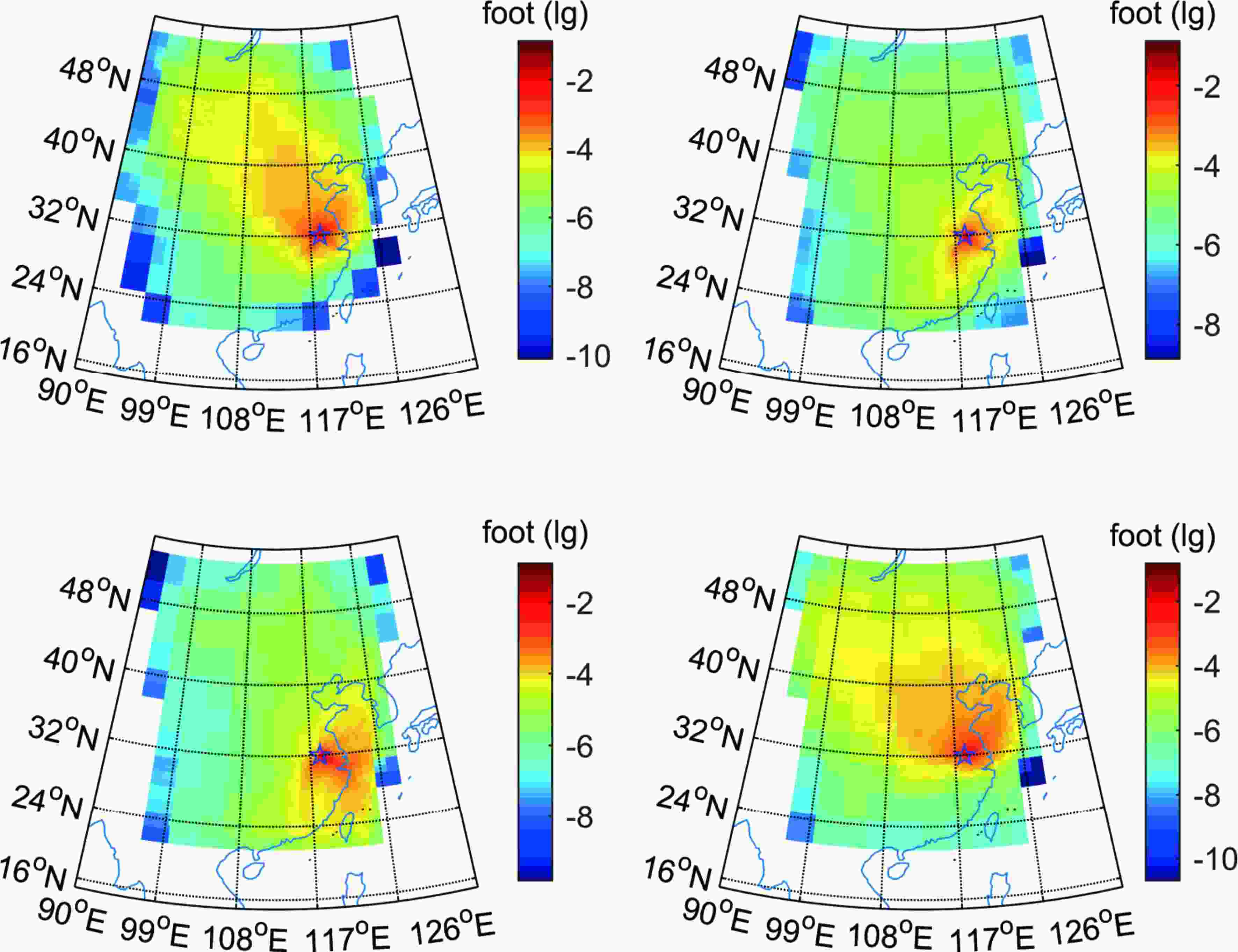 Figure3. Averaged concentration footprint (ppm m2 s μmol?1) for four seasons. (a) Winter (December 2017–February 2018); (b) Spring (March–May 2018); (c) summer (June–August 2018); (d) autumn (September–November 2018). The asterisk represents the location of the observation site.
2
3.2. Simulated CH4 concentration prior to source optimization
Figure 4 compares the hourly and seasonal mean concentration simulated by the model versus the observation. Reasonable agreement between simulated and observed CH4 concentration was achieved for the winter with low temperature (mean air temperature 6.3°C, Fig. 4a), with a mean difference (simulation minus observation) of 99 ppb and 32 ppb and a linear correlation r of 0.56 (p < 0.01) and 0.52 (p < 0.01) for EDGAR v432 and EDGAR v50 prior to optimization, respectively. It should be noted here that due to the abnormality of high CH4 emissions in February and March in EDGAR v432 (section 3.3), the winter correlation coefficient was calculated only with data in December and January and the spring correlation coefficient was calculated only with data in April and May. In the summer (mean air temperature 29.1°C), the simulated values are much lower than the observed values (mean bias error of ?286 ppb for EDGAR v432 and ?213 ppb for EDGAR v50), and the correlation is also weaker than in the wintertime (R2 = 0.21 for EDGAR v432, p < 0.01; R2 = 0.24 for EDGAR v50, p < 0.01; Fig. S4 in the ESM). These patterns suggest that these two inventory databases do not adequately capture the seasonal dynamics of the CH4 sources in the region.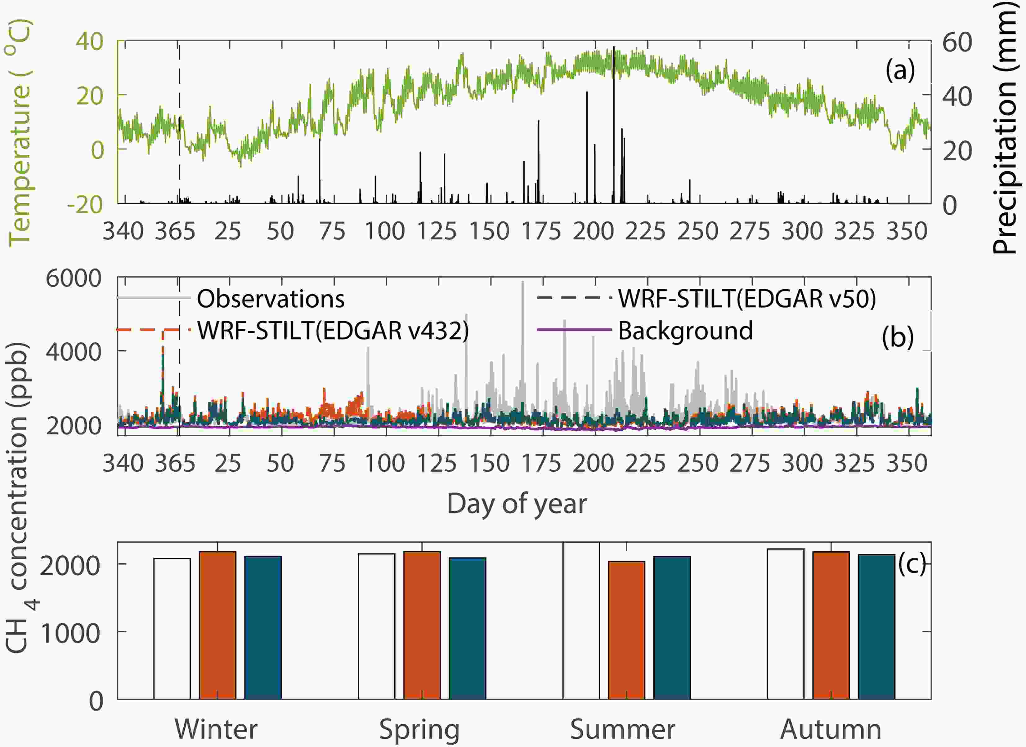 Figure4. Time series of (a) temperature and precipitation, (b) simulated and observed CH4 concentration from December 2017 to December 2018, and (c) seasonal mean simulated and observed CH4 concentration. The black dotted line marks the transition between 2017 and 2018.
The simulated concentration was moderately sensitive to wetland emissions. The seasonal mean concentrations shown in Fig. 4c did not include the concentration enhancement induced by CH4 emission from wetlands. If the wetland emissions were taken into account, the mean bias error (MBE) for the summer improved slightly to ?238 ppb for EDGAR v432 and ?166 ppb for EDGAR v50 from ?286 ppb and ?213 ppb, respectively (Fig. S4). For the summertime simulations, the regression slope of observed and simulated CH4 concentration based on EDGAR v50 was greater than the slope based on EDGAR v432, consistent with the fact that the anthropogenic CH4 emission in EDGAR v50 was reduced from that in EDGAR v432. That large MBE was evident in the summer, even with the inclusion of wetland sources, illustrates the importance of performing the SFBI analyses to optimize the seasonality of CH4 emissions.
2
3.3. Optimization of scaling factors
Tables 1 and 2 summarize the scaling factors obtained with the SFBI method on a monthly basis. In EDGAR v432, CH4 emissions from AGS (agricultural soils) were severely overestimated in February and March, as evidenced by a scaling factor that was much less than 1 (0.36 in February and 0.19 in March). The abnormally high CH4 emissions resulted in a large positive bias in the simulated concentration in this period (Fig. 4b). In comparison, EDGAR v50 gave more reasonable emission estimates for this source category during these months, with no CH4 emissions in February and March. However, both inventories severely understated the AGS emissions during the growing season. The largest underestimation was 274% for EDGAR v432 and 195% for EDGAR v50 in July. Compared with EDGAR v432, EDGAR v50 has improved the seasonal distribution of AGS CH4 emissions throughout the year, which improved the comparison with the observation (Fig. 4c) but was still substantially biased low in the summer.| Time | AGS | PRO | RCO | REF_TRF | SWD_LDF | WWT | Wetlands | ENF | Other |
| Dec 2017 | 0.86 | 0.52 | 0.67 | 0.54 | 0.67 | 0.81 | 0.67 | 0.67 | 0.67 |
| Jan 2018 | 0.94 | 0.39 | 0.76 | 0.75 | 0.76 | 0.85 | 0.76 | 0.76 | 0.76 |
| Feb 2018 | 0.36 | 0.52 | 0.82 | 0.42 | 0.42 | 0.69 | 0.42 | 0.42 | 0.42 |
| Mar 2018 | 0.19 | 0.85 | 0.67 | 0.67 | 0.67 | 0.87 | 0.67 | 0.89 | 0.67 |
| Apr 2018 | 0.70 | 0.98 | 0.75 | 0.75 | 0.75 | 0.91 | 0.96 | 0.75 | 0.75 |
| May 2018 | 1.90 | 1.57 | 1.13 | 1.13 | 1.13 | 1.10 | 1.28 | 1.13 | 1.13 |
| Jun 2018 | 2.00 | 1.51 | 1.63 | 1.63 | 1.63 | 1.31 | 1.33 | 1.63 | 1.63 |
| Jul 2018 | 2.74 | 1.67 | 1.67 | 1.67 | 1.32 | 1.75 | 2.14 | 1.67 | 1.67 |
| Aug 2018 | 2.23 | 1.49 | 1.49 | 1.02 | 1.49 | 1.38 | 2.04 | 1.49 | 1.49 |
| Sept 2018 | 1.61 | 1.19 | 1.49 | 1.00 | 1.49 | 1.15 | 1.49 | 1.49 | 1.49 |
| Oct 2018 | 0.96 | 0.78 | 0.81 | 0.63 | 0.81 | 0.84 | 0.81 | 0.81 | 0.81 |
| Nov 2018 | 0.94 | 0.69 | 0.75 | 0.76 | 0.75 | 0.86 | 0.75 | 0.75 | 0.75 |
| Dec 2018 | 1.04 | 0.56 | 0.75 | 0.52 | 0.75 | 0.81 | 0.75 | 0.75 | 0.75 |
| Notes: AGS—agricultural soils; PRO—fuel exploitation; RCO—energy for building; REF_TRF—oil refineries and transformation industry; SWD_LDF—solid waste landfills; WWT—waste water handling; Wetlands—marshland, mudflats, and water bodies (rivers, lakes, ponds, and reservoirs); ENF—enteric fermentation. Data shown in bold italics are in the “Other” group having the same monthly scaling factor. | |||||||||
Table1. Monthly scaling factors for the main CH4 sources in EDGAR v432.
| Time | AGS | PRO | RCO | REF_TRF | SWD_LDF | WWT | Wetlands | Other |
| Dec 2017 | 0.97 | 0.59 | 0.98 | 0.31 | 0.97 | 0.97 | 0.97 | 0.97 |
| Jan 2018 | 1.10 | 0.38 | 1.04 | 0.64 | 1.10 | 1.04 | 1.10 | 1.10 |
| Feb 2018 | 0.68 | 0.44 | 0.79 | 0.26 | 0.68 | 0.63 | 0.68 | 0.68 |
| Mar 2018 | 0.92 | 0.35 | 0.92 | 0.38 | 0.92 | 0.95 | 1.06 | 0.92 |
| Apr 2018 | 1.67 | 1.33 | 0.65 | 0.65 | 0.65 | 1.23 | 1.28 | 0.65 |
| May 2018 | 1.47 | 1.34 | 0.97 | 0.97 | 0.97 | 1.01 | 1.10 | 0.97 |
| Jun 2018 | 1.36 | 1.13 | 1.17 | 1.17 | 1.17 | 1.04 | 1.00 | 1.17 |
| Jul 2018 | 1.95 | 1.22 | 1.22 | 1.22 | 1.09 | 1.18 | 1.28 | 1.22 |
| Aug 2018 | 1.76 | 1.12 | 1.12 | 0.99 | 1.12 | 1.07 | 1.38 | 1.12 |
| Sept 2018 | 1.80 | 1.33 | 1.57 | 0.96 | 1.57 | 1.13 | 1.57 | 1.57 |
| Oct 2018 | 1.09 | 0.86 | 1.09 | 0.46 | 1.09 | 0.98 | 1.23 | 1.09 |
| Nov 2018 | 0.95 | 0.79 | 0.95 | 0.63 | 0.95 | 1.00 | 1.07 | 0.95 |
| Dec 2018 | 1.19 | 0.57 | 1.02 | 0.36 | 1.19 | 0.98 | 1.19 | 1.19 |
Table2. Monthly scaling factors for the main CH4 sources in EDGAR v50. Refer to Table 1 for source category definition.
CH4 emissions from oil refineries and transformation industry (REF_TRF) were overestimated for the majority of the year. The scale factor for this source category was less than 1 for 8 months (0.52 to 0.76) in the case of EDGAR v432 and for 10 months (0.26 to 0.99) in the case of EDGAR v50.
In generating the wetland emission inventory, we used one emission factor for each season (Table S1 in the ESM). Wetland CH4 emission potential varied through the summer months with a maximum potential observed in July or August. This emission potential is reflected in the SFBI scale factors. The largest scale factor was for July, at 2.14 for EDGAR v432 and 1.38 for EDGAR v50.
The original enhancements based on EDGAR v432 and natural sources did not have reasonable seasonal emission trends compared with the observed concentrations. The highest enhancement came from AGS in the month of March (Fig. S5 in the ESM), which was unreasonable because the temperature was low (13.9°C; Fig. 4a). After applying the SFBI method, AGS was still the most important contributor to the concentration enhancement, but the peak value now occurred in July (Fig. S5), which has the highest monthly mean temperature of 30.3°C. For EDGAR v50, the peak enhancement from AGS changed from June to July after using the SFBI method, and the peak enhancement value changed from 166 ppb to 267 ppb. Another change brought by the SFBI method was the seasonal pattern in the enhancement caused by fuel exploitation (PRO). Originally the PRO enhancement was high in the winter and low in the summer for both EDGAR inventories (Fig. S5). Although the a priori PRO emissions were invariant throughout the year, the prevailing northwest wind in the winter meant that our observational site was heavily affected by emissions in Anhui, which is the only province with coal mining in the YRD, resulting in a large concentration enhancement. After using the scaling factor for PRO (Tables 1 and 2), this seasonality of the PRO enhancement was weakened (Fig. S5).
Figure 5 compares the monthly observed concentration throughout the year with the simulated concentration using different emission configurations. The a priori simulation with EDGAR v432 gave the highest concentration in March (2304.8 ppb) and lowest concentration in July (2046.3 ppb), in sharp contrast to the observed seasonality showing the lowest monthly mean in February (2033.8 ppb) and the highest in August (2379.0 ppb). The a priori simulation with EDGAR v50 displayed a much weaker seasonality (minimum of 2077.2 ppb in March and maximum of 2199.0 ppb in June) than the observed seasonality. After the scale factor adjustments, both the EDGAR v432 and EDGAR v50 posteriori simulations reproduced the observed seasonality quite well. If the AGS source was excluded from the posteriori simulations, the simulated concentration was in the range of 2034.3 ppb to 2156.3 ppb (EDGAR v432) and 2001.8 ppb to 2160.6 ppb (EDGAR v50), much lower than the observed range of seasonal variation. These results indicate that AGS was the main source of the seasonal variation of the atmospheric methane concentration. The simulation results, based on EDGAR v432, showed that the contribution of AGS to total CH4 emissions was lowest in winter (30%) and highest in summer (42%) and was higher than the contribution of natural sources (winter: 2%, spring: 6%, summer: 15%, autumn: 9%). For the EDGAR v50 simulations, the contribution of AGS to total CH4 emissions was 0 in winter and reached the maximum in summer (64%). The contribution of natural sources to total CH4 emissions was the smallest in winter (4%), followed by spring and summer (10%) and the largest in autumn (14%).
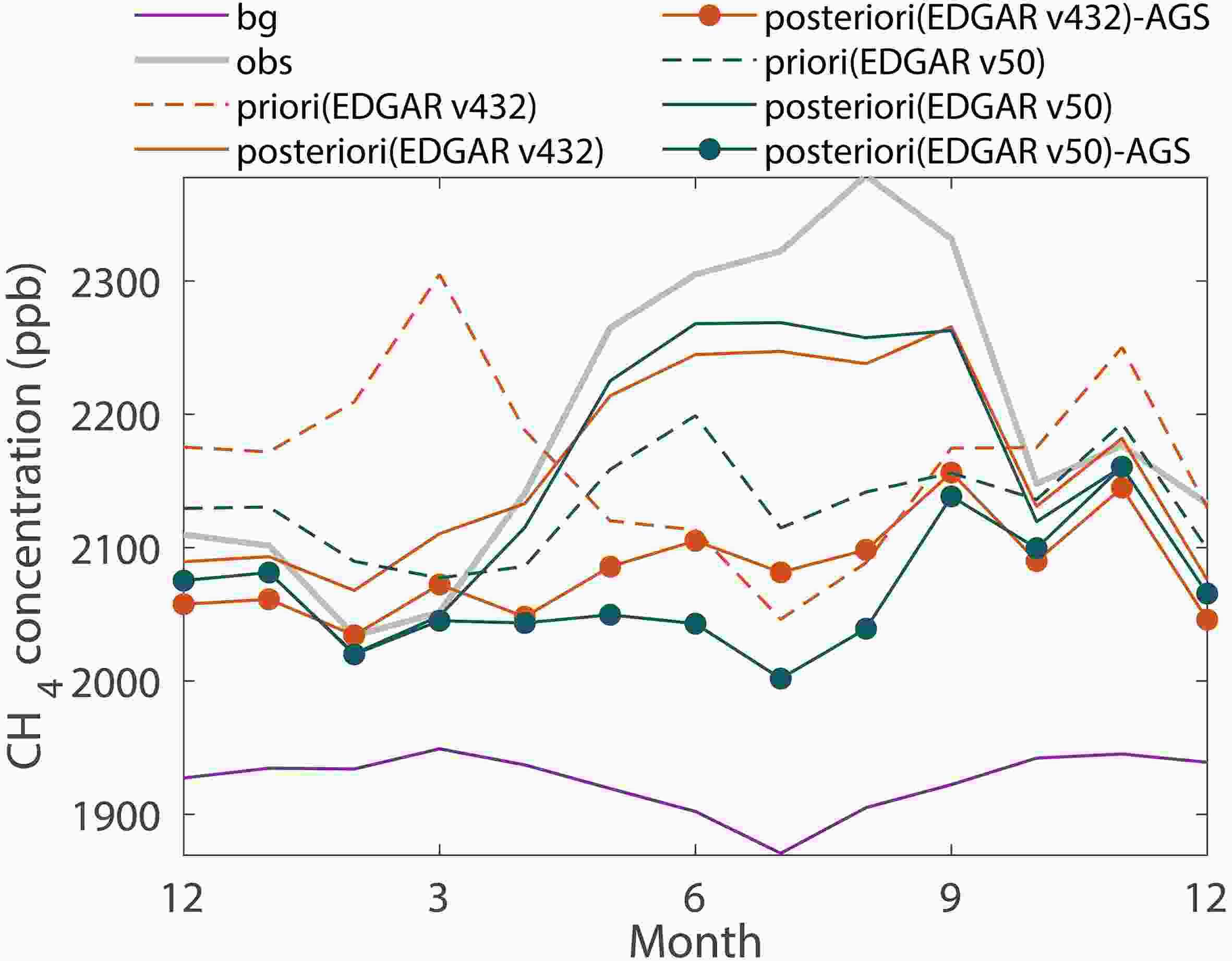 Figure5. Time series of monthly CH4 background concentration (bg), observed concentration (obs), simulated concentrations with a priori and posteriori CH4 fluxes, and simulated concentrations with posteriori CH4 fluxes but excluding emission from agricultural soils (posteriori - AGS).
By applying the scaling factors from Table 1 and Table 2, the slope between the observed CH4 and simulated CH4 concentration enhancement for EDGAR v432 changed from 0.60 to 0.65, and the coefficient of determination R2 increased from 0.05 to 0.40 (Fig. S6 in the ESM). The RMSE were reduced by 25%. Similar results were obtained for the EDGAR v50 simulations. The absolute value of the MBE for EDGAR v432 increased by 36%.
Figure 6 compares the simulated and observed ensemble diel variation of CH4 concentration for the four seasons. The SFBI method improved the simulated diel pattern the most for the summer season, in terms of both the mean value and the diel amplitude. In the other three seasons, the observed and simulated diel amplitudes were weaker, and the improvement brought by the SFBI appeared as a reduction of the MBE. Both a priori and posteriori simulations produced a diel peak value at about 0600 LST in the summer and in the autumn, which was 1 to 2 h ahead of the observed diel cycle (Figs. 6c and 6d). Some of the time mismatch may have been a result of inaccurate PBLH diel variations. The PBLH simulated by WRF has the lowest value at 0700 LST in the winter, and the PBLH was lowest at 0600–0800 LST in the autumn. The timing of these simulated peaks may have been too early in comparison to the limited wind profiler observations (Fig. S7 in the ESM).
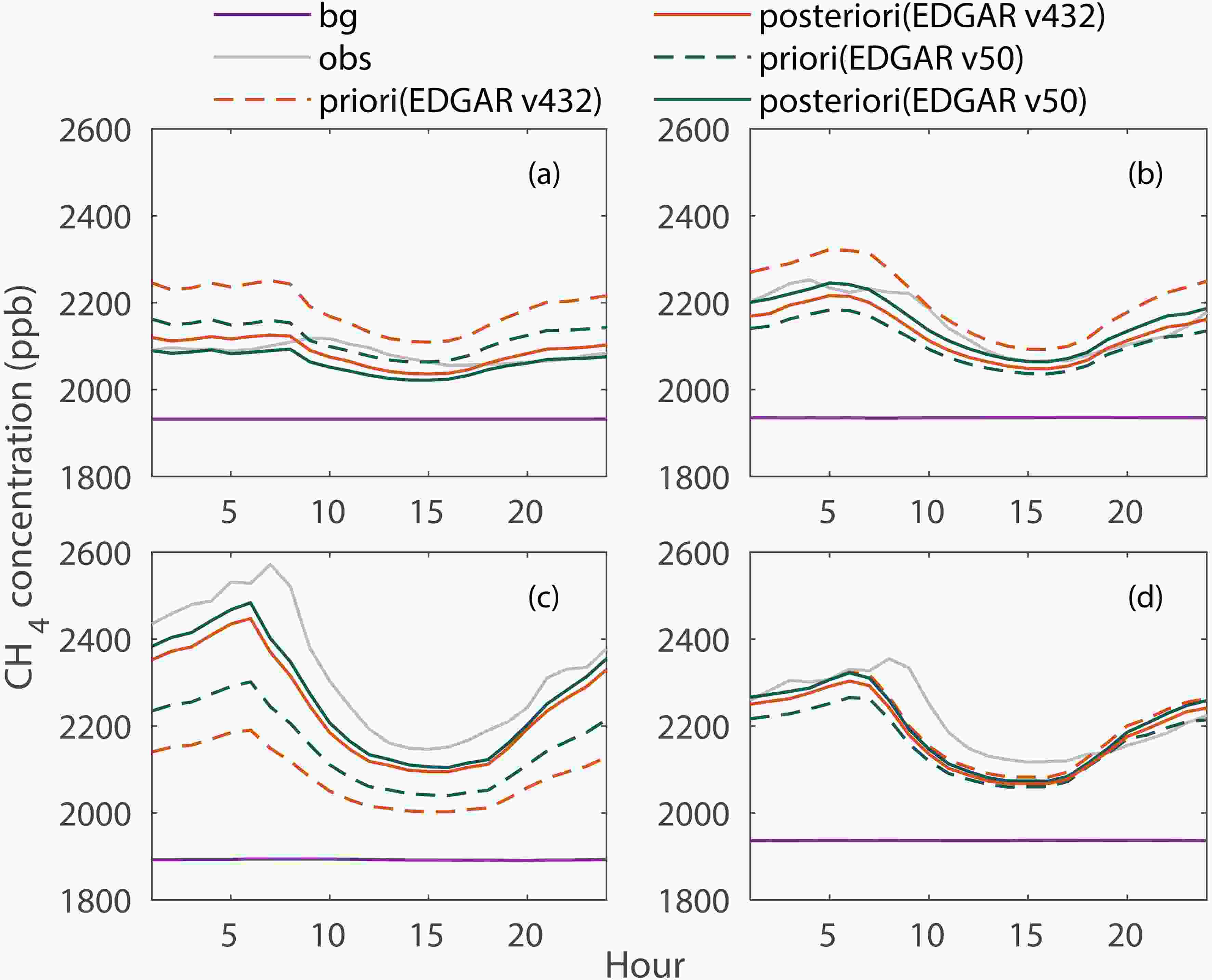 Figure6. Ensemble diel variation of CH4 concentration in (a) winter, (b) spring, (c) summer, and (d) autumn.
2
3.4. A priori and posteriori CH4 flux by source category
Tables S2 and S3 (in the ESM) compare the a priori and posteriori CH4 emissions for the major source categories in the YRD on a monthly time scale in 2018. We first examine the wetland emission. This source category is broadly defined to include marshland, mudflats, and water bodies (rivers, lakes, ponds, and reservoirs). Recall that the a priori emission factors (flux density, emission per unit time per unit wetland surface area) for the natural wetland sources were the same for each season, with the highest flux density of 128.01 nmol m?2 s?1 in summer and the lowest flux of 15.86 nmol m?2 s?1 in winter (Table S1 in the ESM). Considering that the regional flux of each source obtained from EDGAR products is total emission per unit time divided by the total YRD area, it is necessary to multiply the wetland flux density by the percent of water body and marshland area in the YRD (7.13%, according to the land use statistics, consisting of 0.22% marshlands and 6.91% water bodies; section 2.1) to estimate the a priori regional emission for wetlands. After optimization, the regional wetland emission varied on the monthly time scale, peaking in August at 19.52 nmol m?2 s?1 and 12.62 nmol m?2 s?1, when other sources were constrained by EDGAR v432 and v50 as a priori inventories, respectively. A similar peak monthly regional flux of 17 nmol m?2 s?1 has been reported by Chen et al. (2018) for the U.S. Midwest using the WRF-STILT inverse modeling strategy. The high regional wetland flux in July and August (Fig. S8 in the ESM) appeared to be related to key climate drivers. These two months experienced the highest and second highest monthly temperature (30.3°C in July and 29.9°C in August) and monthly precipitation (181 mm in July and 304 mm in August, Fig. 4a). These conditions are known to favor methanogenesis and CH4 production (Bridgham et al., 2006; Melton et al., 2013).Our wetland result can be compared with two bottom-up estimates for the YRD region found in the literature. Our estimates of the annual mean regional wetland flux, 6.60 nmol m?2 s?1 and 5.80 nmol m?2 s?1 according to optimized EDGAR v432 and EDGAR v50, respectively, are about two to three times the annual mean reported by Bloom et al. (2017) for wetlands in the YRD region. In Bloom et al. (2017), wetland emission was calculated at a grid resolution of 0.5° × 0.5° using an ensemble approach consisting of multiple parameterizations of wetland extent, heterotrophic respiration, and temperature sensitivity. Data from Bloom et al. (2017) also indicate a higher wetland flux in the warm season than in the cold season, but differ from our estimates in two details. First, their peak emissions occurred in June, whereas our peak values occurred in July or August. Second, the peak monthly value is much smaller than ours (Fig. S8 in the ESM). A literature survey by Zhang and Jiang (2014) of CH4 flux observations in 14 wetlands in China reveals that these wetlands vary from a weak sink (flux density ?1.04 nmol m?2 s?1) to a strong emission source (flux density 781.25 nmol m?2 s?1). Their best estimate of the annual mean flux density for wetlands in Central China, which includes the YRD region, is 38 nmol m?2 s?1. Their flux density is expressed on the basis of unit wetland surface area. Recalling that wetland fraction in the YRD is about 7.13%, the annual flux density found by Zhang and Jiang (2014) is equivalent to a regional CH4 flux of 2.71 nmol m?2 s?1, which is about half of our posteriori estimates. The disparity between the top-down and bottom-up wetland emission estimate exists largely because of the high spatial variability of emissions from natural sources, differences among measurement techniques, and the overall scarcity of direct flux measurements (Ito and Inatomi, 2012; Wei and Wang, 2016, 2017; Ito et al., 2019). However, combining these top-down and bottom-up methods can give guidance on how to best optimize emission estimates from natural sources (Verhulst et al., 2017; Kunik et al., 2019).
Agricultural soils (AGS) is another source category that deserves expanded discussion. Since field measurements generally express the CH4 emission as a flux density, here we converted the spatially averaged flux (Table S3 in the ESM and Table 3) to the flux density by dividing the regional flux with the rice paddy areal percent of 15.35% (section 2.1). Agricultural statistics show that 90% of the rice grown in the YRD is medium- and late-season rice (National Bureau of Statistics, 2018). To further facilitate comparison with observational studies, we partitioned the annual flux density to growing-season and nongrowing-season values assuming a growing season from 17 June to 14 October (length of 120 days). The results are given in Fig. S9 (in the ESM) and Table 4.
| Anthropogenic source: agricultural soils | All anthropogenic sources | Wetlands | Total | ||
| EDGAR v432 | a priori | 4.01±1.49 | 10.08±1.76 | 0.87±0.33 | 10.96±1.79 |
| posteriori | 4.58±1.37 | 10.68±1.63 | 1.21±0.48 | 11.89±1.71 | |
| EDGAR v50 | a priori | 3.17±1.49 | 8.16±1.68 | 0.87±0.33 | 9.04±1.72 |
| posteriori | 5.21±1.53 | 10.07±1.67 | 1.06±0.39 | 11.13±1.71 |
Table3. CH4 emissions in the YRD in 2018 (units: Tg CH4).
| Growing season | Non-growing season | Annual | ||
| EDGAR v432 | a priori | 132.7 | 149.3 | 144.4 |
| posteriori | 270.2 | 112.5 | 163.8 | |
| EDGAR v50 | a priori | 222.0 | 60.6 | 113.0 |
| posteriori | 389.3 | 87.5 | 185.5 |
Table4. Seasonal and annual mean CH4 flux density (units: nmol m?2 s?1) from agricultural soils (AGS). Flux density is defined as emission per unit time per unit area of agricultural soils.
The posteriori AGS flux density had much more reasonable seasonality than the a priori flux density (Fig. S9 in the ESM). After applying the SFBI method, the flux density peaked in July, during the middle of the rice growing season in the YRD (mid-June to mid-October). Zou et al. (2005) also observed that the highest flux density occurred in early July after rice transplanting. Their field experiment was conducted in the rice phase of a typical wheat-rice rotation field in Jiangsu Province. Kong et al. (2019) observed a sharp drop in CH4 flux that lasted for a week during the mid-season drainage at the end of the tillering period in August. This water management regime is commonly used in other regions of China except the southwest (Shi et al., 2010). This may be part of the reason why CH4 flux from AGS in August was lower than in July (Fig. S9). Under the policy of banning straw burning and government subsidies for returning straw to the field, increased demand for food production has promoted the use of fertilizer and returning straw to rice fields in China. Therefore, the CH4 flux from AGS in July for the tillering stage is expected to have an increasing trend in the YRD (Cai et al., 2007; Fan et al., 2016). Wang et al. (2015) reported that the flux density peaked in August in a late season rice crop in Fujian Province, a province at the southern boundary of the YRD. Using a process model that integrates the distribution of rice paddies, rice calendar, climate, and soil conditions, Cao et al. (1996) showed that in the rice growing regions at latitudes north of 20°N, the highest flux density occurs between July and September.
Previous field-based measurements (e.g., chambers, eddy covariance) of CH4 emissions from rice have mainly been conducted during the growing season (e.g., Cai et al., 1999; Khan et al., 2015). The growing season flux density was 132.7 nmol m?2 s?1 and 222.0 nmol m?2 s?1 in EDGAR v432 and EDGAR v50, respectively. These values were adjusted upward to 270.2 nmol m?2 s?1 and 389.3 nmol m?2 s?1 after applying the SFBI method (Table 4). The adjusted flux densities were higher than the growing season flux density of 211.8 nmol m?2 s?1 reported by Shi et al. (2010) for rice paddies in the middle and lower reaches of the Yangtze River. The process model of Cai (1997) yielded a growing season mean flux density of 184.5 nmol m?2 s?1 for rice paddies in the latitudinal range of 20°–30°N, which is also much lower than our posteriori estimates for AGS. These differences may be related to the promotion of management practices that return straw residues to the field in recent years. By 2014, straw fertilization had reached 35% in China (Editorial Committee of China Agricultural Yearbook, 2015). The estimate by Shi et al. (2010) is based on a meta-analysis of observational studies made before 2009 when retention of crop residues was not a common farming practice. The application of wheat straw in Nanjing, China, increased the CH4 flux density by 250% during the rice-growing season (Zou et al., 2004). The CH4 flux density peaked at 1644.1 nmol m?2 s?1 and 293.4 nmol m?2 s?1 with and without straw application, respectively, in a late-season rice field in southeastern China (Wang et al., 2015). Incorporation of crop straw into the soil increased the seasonal total emission by 3.6 to 5.5 times in comparison to the conventional management practice that disposed of crop straw offsite, in a paddy field in subtropical central China (Wang et al., 2017).
2
3.5. Regional CH4 budget in 2018
The total regional CH4 emission from the YRD in 2018 was 10.96 ± 1.79 Tg and 9.04 ± 1.72 Tg according to EDGAR v432 and EDGAR v50, respectively (Table 3). The proportion of AGS contribution was 37% and 35%, respectively. The uncertainties of these results were based on the Monte Carlo method.After applying the SFBI, the total regional emission was 11.89 ± 1.71 Tg and 11.13 ± 1.71 Tg according to EDGAR v432 and EDGAR v50, respectively. Emission from AGS accounted for 39% (4.58 Tg, EDGAR v432) and 47% (5.21 Tg, EDGAR v50) of the total emission. PRO (fuel exploitation) and WWT (wastewater handling) were two other dominant anthropogenic emission sources, accounting for 35% (EDGAR v432, 3.70 Tg) and 27% (EDGAR v50, 2.72 Tg) of the anthropogenic emission subtotal and 31% (EDGAR v432) and 24% (EDGAR v50) of the regional total emission. The proportion of natural wetland emission to the regional total was ~10% (1.21 Tg in EDGAR v432 and 1.06 Tg in EDGAR v50).
The seasonal characteristics of the CH4 budget (Fig. 7) can largely explain why our regional total (11.89 Tg and 11.13 Tg) was higher than 6.52 ± 1.59 Tg obtained by Hu et al. (2019) for the YRD in the calendar year 2011. Their estimate, which did not consider wetland contributions, was obtained with the same inverse model using EDGAR v432 as a priori emission, but the model was constrained with concentration observations made in the cold season (November 2020 to April 2011) at a different site (about 50 km to northeast of our site). They found that the posteriori anthropogenic CH4 flux (36.0 nmol m?2 s?1) was 31% lower than the priori anthropogenic CH4 flux (52.1 nmol m?2 s?1). Similarly, in this study the posteriori anthropogenic flux (38.8 nmol m?2 s?1) for the period from November to April 2018 was 36% lower than that (60.7 nmol m?2 s?1) obtained from EDGAR v432 after the annual growth adjustment from 2011 to 2018 (Fig. 7a). Extrapolating our posteriori cold-season anthropogenic flux values to the full year, we obtained an annual regional emission total of 7.05 Tg (EDGAR v432), in close agreement with Hu et al. (2019)’s estimate, especially if we accounted for the annual growth rate of anthropogenic CH4 emission in the YRD region (2% yr?1; section 2.3). While using EDGAR v50 as a priori emission, an annual regional emission total of 5.02 Tg was smaller than 7.05 Tg achieved by EDGAR v432. This difference was mainly attributed to a priori AGS. In EDGAR v50, during half of the cold-season (November–January), the emissions for AGS were 0, and the emissions for the remaining three cold months were also very small (4.92 nmol m?2 s?1). However, the a priori emissions for AGS in EDGAR v432 are overestimated in February and March, with the emissions of AGS for the cold-season period being 8.72 nmol m?2 s?1. Therefore, when the annual regional emissions total was estimated only based on the anthropogenic CH4 flux during the cold season, the results had a large deviation.
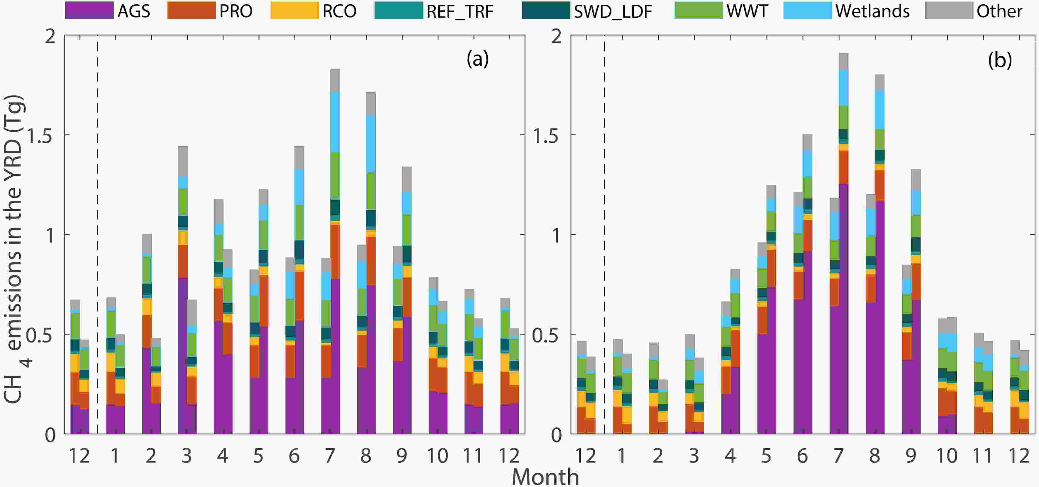 Figure7. Comparison of a priori (left column) and posteriori (right column) monthly emission total on (a) EDGAR v432 and (b) EDGAR v50. Refer to Table 1 for source category definition.
Our results also highlight the role of rice paddies in regional CH4 budgets. It remains difficult to extrapolate field-scale experimental data to assess national total emissions on an annual scale. Zou et al. (2009) classified five major rice regions in China. Shi et al. (2010) obtained typical CH4 flux estimates for these regions by conducting a meta-analysis of field experimental results. Combining the areas of these five regions as weighting factors (National Bureau of Statistics, 2018), the weighted average CH4 flux was taken as China's average flux (10.88 mg m?2 h?1). This flux estimate was compared with that of the Middle and lower Yangtze River rice planting area (12.59 mg m?2 h?1) to obtain a conversion factor (10.88/12.59=0.86). We used this conversion factor to upscale the CH4 flux in the YRD obtained in our study to estimate the CH4 flux for all of China. The difference in rice growing days (from transplanting to harvesting) in each region was not considered. The average value (representing 115 days) in the integrated database was selected by default (Shi et al., 2010). As a result, the upscaled CH4 emissions during the rice growing season (representing 120 d) in China (rice area 3.02 × 10¹¹ m2; National Bureau of Statistics, 2018) were 11.67 Tg and 16.82 Tg according to the optimized EDGAR v432 and EDGAR v50, respectively. The corresponding annual rice emission was 21.52 Tg (EDGAR v432) and 24.37 Tg (EDGAR v50). Based on a bottom-up method, Peng et al. (2016) estimated that the CH4 emissions from rice paddies in China in 2010 were 7.4 ± 1.4 Tg, accounting for 16% of anthropogenic CH4 emissions. The large disagreement may be related to methodological differences between top-down and bottom-up approaches and also raises the possibility that recent changes in agricultural practices, such as retaining crop residues in rice paddies, may have unintended climate consequences.
1. The main factor causing seasonal changes in atmospheric CH4 concentration in the Yangtze River Delta was rice cultivation.
2. The posteriori anthropogenic emissions of the whole region were 10.68 ± 1.63 Tg and 10.07 ± 1.67 Tg when using EDGAR v432 and EDGAR v50 as priori emissions, respectively.
3. Among anthropogenic emissions, the proportion of AGS ranged from 42.9% (using EDGAR v432 as a priori emission) to 51.7% (using EDGAR v50 as a priori emission). The posteriori emissions from natural sources (including wetlands and water bodies) were 1.21 ± 0.18 Tg and 1.06 ± 0.39 Tg in YRD in 2018.
4. The underestimation of the anthropogenic CH4 emissions in the YRD from the inventory products was mainly caused by the underestimation of emissions from rice cultivation, especially during the growing seasons.
5. For anthropogenic sources other than AGS, the deviation between the a priori emission and the posteriori results was small (0.03 Tg for EDGAR v432 and ?0.13 Tg for EDGAR v50).
Acknowledgements. This work was supported by the National Key R&D Program of China (Grant Nos. 2020YFA0607501 and 2019YFA0607202 to WX), the Natural Science Foundation of Jiangsu Province (Grant No. BK20200802 to CH), and the Key Laboratory of Meteorology and Ecological Environment of Hebei Province (Grant No. Z201901H to WX). We are grateful to all of the staff who work at the WMO/GAW stations for collecting the data, and to the Greenhouse Gases Research Laboratory of the China Meteorological Administration (CMA) for data analysis. We appreciate all of the staff who work at NOAA, Japan Meteorological Agency (JMA), and Viet Nam Meteorological and Hydrological Administration (VNMHA) for their help and support of the research measurements. The data used in this study are available at
Electronic supplementary material: Supplementary material is available in the online version of this article at
