Isidora JANKOV^1,,,
Scott GREGORY²,
Sai RAVELA³,
Zoltan TOTH¹,
Malaquías PE?A⁴

Corresponding author: Isidora JANKOV,Isidora.Jankov@noaa.gov;

1.Global Systems Laboratory, NOAA/OAR, Boulder, CO 80305, USA
2.General Atomics, Electromagnetic Systems Group, Longmont, CO 80501, USA
3.Earth Signals and Systems Group, Earth, Atmospheric and Planetary Sciences, Massachusetts Institute of Technology, Cambridge, MA 02139, USA
4.Department of Civil and Environmental Engineering University of Connecticut, Storrs, CT 06269, USA
Manuscript received: 2020-07-28
Manuscript revised: 2021-02-09
Manuscript accepted: 2021-02-18
Abstract: Weather manifests in spatiotemporally coherent structures. Weather forecasts hence are affected by both positional and structural or amplitude errors. This has been long recognized by practicing forecasters (cf., e.g., Tropical Cyclone track and intensity errors). Despite the emergence in recent decades of various objective methods for the diagnosis of positional forecast errors, most routine verification or statistical post-processing methods implicitly assume that forecasts have no positional error. The Forecast Error Decomposition (FED) method proposed in this study uses the Field Alignment technique which aligns a gridded forecast with its verifying analysis field. The total error is then partitioned into three orthogonal components: (a) large scale positional, (b) large scale structural, and (c) small scale error variance. The use of FED is demonstrated over a month-long MSLP data set. As expected, positional errors are often characterized by dipole patterns related to the displacement of features, while structural errors appear with single extrema, indicative of magnitude problems. The most important result of this study is that over the test period, more than 50% of the total mean sea level pressure forecast error variance is associated with large scale positional error. The importance of positional error in forecasts of other variables and over different time periods remain to be explored.
Keywords: forecast error,
orthogonal decomposition,
positional,
structural
摘要:天气系统显示出时空连续的结构。因此，天气预报受到位置误差和结构（或振幅）误差的影响。预报员很早就已经认识到这个问题了（例如对于热带气旋的路径和强度的预报误差）。尽管最近几十年，已经有一些客观的方法用于对位置相关的预报误差进行诊断，大多数常规的检验或者统计后处理方法仍然假定预报中不存在位置相关的误差。本文提出了一种预报误差分解的方法（Forecast Error Decomposition, FED），该方法利用场调整的技术，将一个格点的预报场向其对应的分析场进行调整。利用这种方法可以将总误差分解成三个正交分量：（a）大尺度位置误差，（b）大尺度结构误差，和（c）小尺度误差。将FED方法应用于一个月的平均海表气压数据。结果显示，位置误差呈现偶极型，和特征的位置偏移有关，而结构（振幅）误差呈现单极型，表征了特征的振幅偏差。该研究中最重要的结果就是在试验的时长内，海表气压预报的总误差方差有50%以上和大尺度的位置误差有关，说明了预报中的位置误差的重要性。其它变量和其它时间段的预报误差的分解和位置误差的比重还需要进一步的研究。
关键词:预报误差,
正交分解,
位置误差,
结构误差

HTML

--> --> -->

Assessing the quality of forecasts is critical to the development and proper use of Numerical Weather Prediction (NWP) systems. Traditional approaches use univariate methods comparing forecasts with verifying data independently at a set of observation sites or grid-points (i.e., error variance—EV, or root mean square error—RMSE), implicitly assuming that NWP errors are spatially independent. This assumption goes against basic synoptic experience that weather manifests in spatiotemporally organized structures.
Such synoptic observations about the organization of weather systems have motivated decades-long efforts to separate and operationally utilize the positional (e.g., location of central pressure or track) and amplitude (i.e., value of central pressure, or intensity of maximum winds, Goerss and Sampson, 2004; Goerss, 2007; Kehoe at al., 2007) errors associated with Tropical Cyclones (TC, see, e.g., Colby, 2016). Errors in the central position of TCs can be further decomposed into along and across track errors (Buckingham et al., 2010). More recently, similar statistics have also been evaluated for extratropical cyclones (e.g., Colle and Charles, 2011).
Motivated by the decomposition for TC errors, the past decades saw the emergence of a number of other feature-based approaches. These studies include the object-oriented approach of Ebert and McBride (2000), Nachamkin (2004), and Davis et al. (2006), as well as a study by Wernli et al. (2008) that focuses on small regions around selected features to determine structure, amplitude, and location related error statistics.
Other studies take a more systematic approach to forecast error decomposition. These use field deformation (also referred to as optical flow) to smoothly deform one field to align it with another, e.g. verification field. In its verification applications, field deformation is used to decompose full 2D forecast error fields (as opposed to only errors related to selected features). A study by Hoffman et al. (1995), further discussed in the next section, and the correlation and variational optic-flow-based technique of Keil and Craig (2007) is an example of this type of approach. The field deformation concept was first developed and used for other applications (e.g., data fusion—Mariano, 1990; hurricane relocation—Hoffman et al., 1995; bias correction—Nehrkorn et al., 2003; and data assimilation—Lawson and Hansen, 2005; Ravela et al., 2007; Beechler et al., 2010).
In this study, a new method called Forecast Error Decomposition (FED) is introduced, using the Field Alignment (FA) technique of Ravela (Ravela, 2007; Ravela et al., 2007). FA and its application in FED are introduced in section 2. The experimental data and setup are described in section 3, while FED application results are shown in Section 4. section 5 offers a brief summary and a discussion of the characteristics of the approach.

One of the first studies that attempted to formally decompose 2D forecast error fields into positional and other components is Hoffman et al. (1995). Their method concurrently aligns the forecast field (i.e., moves its features across a coarse grid), and adjusts its amplitudes to minimize the difference between the aligned and adjusted forecast field and the verifying observations or analysis field. Displacement and amplitude errors are related to the positional alignment and amplitude adjustment respectively, while the remaining difference between the aligned and adjusted forecast and observations or verifying analysis is called “residual” error that is a function of the smoothing parameters used in the method. Even though the method of Hoffman et al. (1995) provides a conceptual error decomposition, it requires the posterior (i.e., after alignment) forecast error covariance as an input, making its application problematic.

2

-->

2.1. Field Alignment

As Hoffman et al. (1995) point out, there is no unique way of defining forecast displacement errors. In this study, we test the use of an alternative technique, the FA technique (Ravela et al., 2007) in FED. FA and its variants in the Field Alignment System and Testbed (FAST, Ravela, 2007; Ravela et al., 2007) align two gridded fields (in its FED application, a forecast with its verifying analysis field) by smoothly remapping the coordinate system underlying the state of a variable. For example, for two 2D fields of a state variable (e.g. surface temperature), where one field is the observed or analyzed field (which would be considered as the target state) and the other one is a forecast of that field valid at the same time, the FA method estimates a smooth 2D displacement vector field that aligns the forecast with the analysis field. If the displacement vectors are applied to each grid point of the original forecast field as a translation operation in 2D space, the result is an adjusted forecast field for which the difference in RMSE between this aligned field and the analysis field (i.e., cost function) is minimized. The displacement vector field and the aligned field are derived through a variational minimization of the cost function in FA (Ravela, 2007). The smoothness of the displacement vector field is controlled via a “smoothness wavenumber parameter” (SWP) in the FA truncation algorithm (Ravela, 2012). SWP defines the scales at which alignments of features between two fields are performed. Smaller scale features are moved along with the larger scale features that are aligned, without additional adjustments. SWP is the only free parameter in FA and it is analogous to the choice of truncation in Hoffman et al.’s (1995) approach.
Unlike the method proposed by Hoffman et al. (1995), FA does not rely on forecast error covariance information. For additional details on how FA differs from the method of Hoffman et al. (1995), see Ravela et al., 2007; and Ravela, 2014. As for other FA applications, Ravela (Ravela, 2007; Ravela et al., 2007) and Williams (2008) align the first guess forecast field with the latest observations before the application of a standard data assimilation scheme. This pre-processing reduces the remaining, mostly amplitude errors for a further improvement in the fit to the observations. FA has also been used to analyze (with ensemble-based analysis approaches, Ravela et al., 2009; Ravela, 2012, 2014) and represent (e.g., Ravela et al., 2009) coherent structures in other fluid applications. Additionally, FA has been found to be an effective tool for nowcasting (Ravela, 2012, 2014), initialization, verification (Ravela et al., 2007; Ravela, 2014), and various other applications (Yang and Ravela, 2009a,b; Ravela, 2015a, b).

2 -->

2.2. Forecast Error Decomposition

The purpose of this study is to demonstrate the use of the FA technique in FED for the quantification of what is subjectively perceived as major modes of error. In our study, we will use Error Variance (EV, or on some figures, its root, the Root Mean Square error—RMS) as traditional, scalar references measuring the difference between two 2D fields. The total forecast error variance (E_t) is defined as a difference between forecast (F) and analysis (A) fields. A displacement operator (D) adjusts the forecast field to a new, aligned state (F_a) for which the difference in RMSE between the forecast field (F) and the analysis (A) is minimized. The displacement operator generates both the displacement vector field and the scalar field of the magnitude of displacement.
As pointed out in section 2.1, only large scale features of F are aligned with similar features in A. Correspondingly, positional (P_ls) and structural (S_ls) errors in F will also be defined for the large scales. To calculate large scale positional and structural errors, we first smooth fields F, F_a, and A with the moving average method, using 5 points as the smoothing parameter. The level of smoothing (over 5 points) was chosen so the lines defined by F^s–$F_{{\rm{a}}}^{\rm{s}} $ and $F_{{\rm{a}}}^{\rm{s}} $ are approximately orthogonal. To ensure orthogonality between large scale positional and large-scale structural errors, F^s–$F_{{\rm{a}}}^{\rm{s}} $, we introduce $F_{{\rm{a}}}^{\rm{s'}} $ (adjusted smoothed aligned forecast) as the point closest to A^s (see the schematic in Fig. 1). Note that since $F_{{\rm{a}}}^{\rm{s'}} $ lies on a line defined by two smoothed fields (F^s–$F_{{\rm{a}}}^{\rm{s}} $), this field itself is composed of large scales only, without any additional filtering.
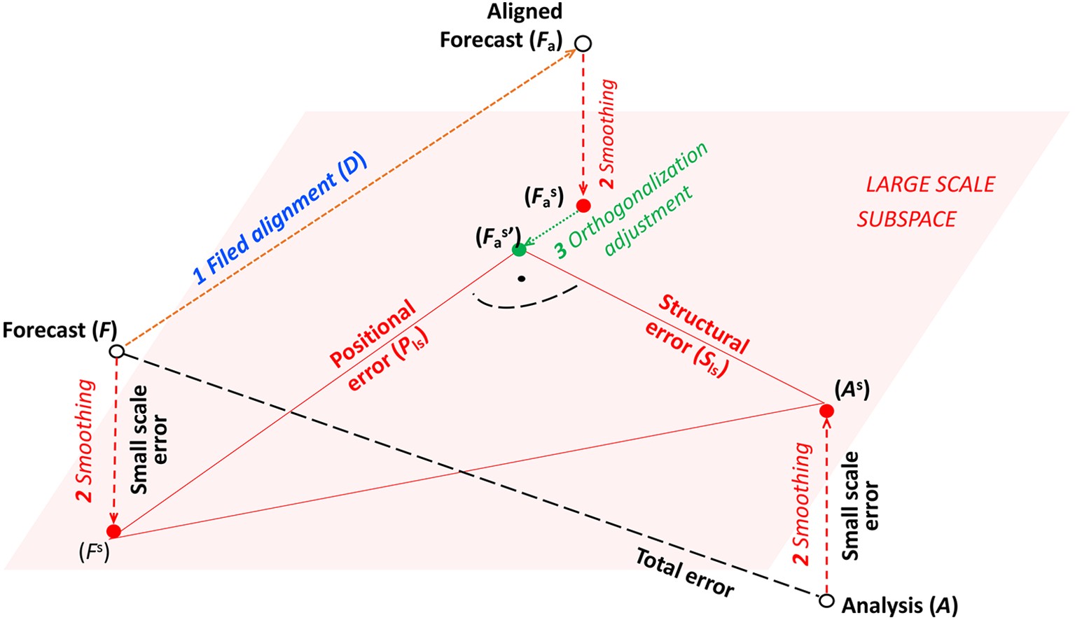Figure1. Schematic of a forecast, verifying analysis, and aligned forecast (open black circles) situated in the phase space of full atmospheric variability, shown in 3D here. Smoothed versions of these fields (solid red circles) reside in the subspace of large scale atmospheric variability, represented with a plane. The orthogonally adjusted smoothed aligned forecast (green solid circle) is defined as a point on the Forecast – Aligned Forecast line in the large scale subspace closest to the Analysis. Large scale positional, large scale structural, and small scale error variances are defined as the variance distance between Forecast and Aligned Forecast, and Aligned Forecast and Analysis in the large scale subspace, and the sum of the variance distances between the original and smoothed Analyses, and the original and smoothed Forecasts, respectively. For further discussion, see text.


Large scale positional and structural errors are then defined as F^s–$F_{{\rm{a}}}^{\rm{s'}} $, and $F_{{\rm{a}}}^{\rm{s'}} $–A^s, respectively. Total error is thus decomposed into three orthogonal components: large scale positional and structural errors and small scale error, the latter of which is orthogonal to the large scale error components as it resides in a different part of the spatial spectrum. Small scale error variance then can be determined either as the difference between total error variance and large scale error variance (i.e., the sum of large scale positional and large scale structural error variance), or as the sum of the differences A–A^s, and F–F^s.

The Forecast Error Decomposition (FED) method described in section 2 is demonstrated using the National Centers for Environmental Prediction (NCEP) Global Ensemble Forecasting System (GEFS, Toth and Kalnay, 1993; Zhu et al., 2012) with 0.5 degree horizontal grid spacing, along with Global Forecast System (GFS) analysis fields given on the same grid. The GEFS forecast uncertainty is determined by generating an ensemble of multiple (21) forecasts where both the initial conditions (Ensemble Transform with Rescaling – ETR, Wei et al., 2008) and the model integrations (stochastic noise, Hou et al., 2006) vary. GEFS global forecasts are produced four times a day, with each run extending out to 16 days. The most recent gridded forecast data and corresponding analyses are available through the NOAA National Operational Model Archive and Distribution System (NOMADS, Alpert et al., 2002, https://nomads.ncep.noaa.gov/).
In this study, FED has been applied to Mean Sea Level Pressure (MSLP) and 850 hPa temperature forecasts of the unperturbed (or control) member of the GEFS initialized at 0000 UTC during the period 1 to 30 September, 2011. This period was characterized by two tropical storms (Lee and an unnamed storm), two category one hurricanes (Maria and Nate), and two category four hurricanes (Katia and Ophelia) in the Atlantic Basin.

We first demonstrate FED using an 84 h forecast initialized at 0000 UTC 9 March 2011. On this day hurricane Katia (2011) was located in the Caribbean area, classified as a category 3 hurricane, with maximum sustained wind speeds between 49.62 m s^-1 and 62.14 m s^-1. Therefore, we focus on a domain covering a portion of the Northern Atlantic Ocean basin. Figure 2 shows the GFS analysis and the control (unperturbed) GEFS 84 h MSLP forecast valid at the same time. The forecast storm (Fig. 2b) lags behind the analysis both in terms of its location and its intensity.
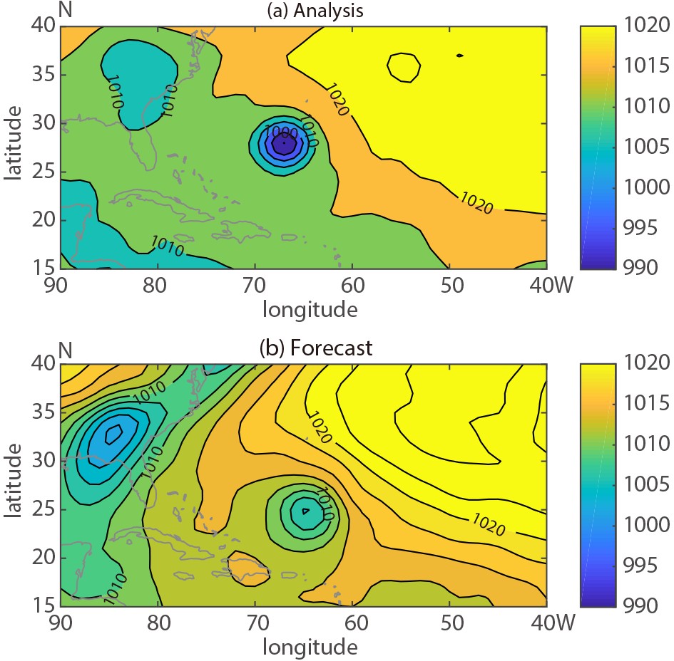Figure2. GEFS control member 84 h forecast and the GFS analysis valid at 1200 UTC September 6, 2011.


The decomposition of the error for the same 84-hour forecast is shown in Fig. 3, with total error as a difference between the original forecast and the verifying analysis field (a), the displacement vector field as defined by the difference in the position of the original and aligned forecast fields (b), the large scale positional error as a difference between the smoothed forecast and the adjusted smoothed aligned forecast fields (c), the large scale amplitude error as a difference between the adjusted smoothed aligned forecast and the smoothed analysis fields (d), and the small scale error as the difference between the total error and total error for large scales. For clarity, the displacement vector field (Fig. 3b) has been scaled and the data have been thinned (represented only at every 2nd grid point). In the tropical Atlantic, the magnitude of the displacement vectors is largest over and around the hurricane itself (Fig. 3b). The structure of the vector field indicates an error related to an along-track delay in the forecast movement of the storm.
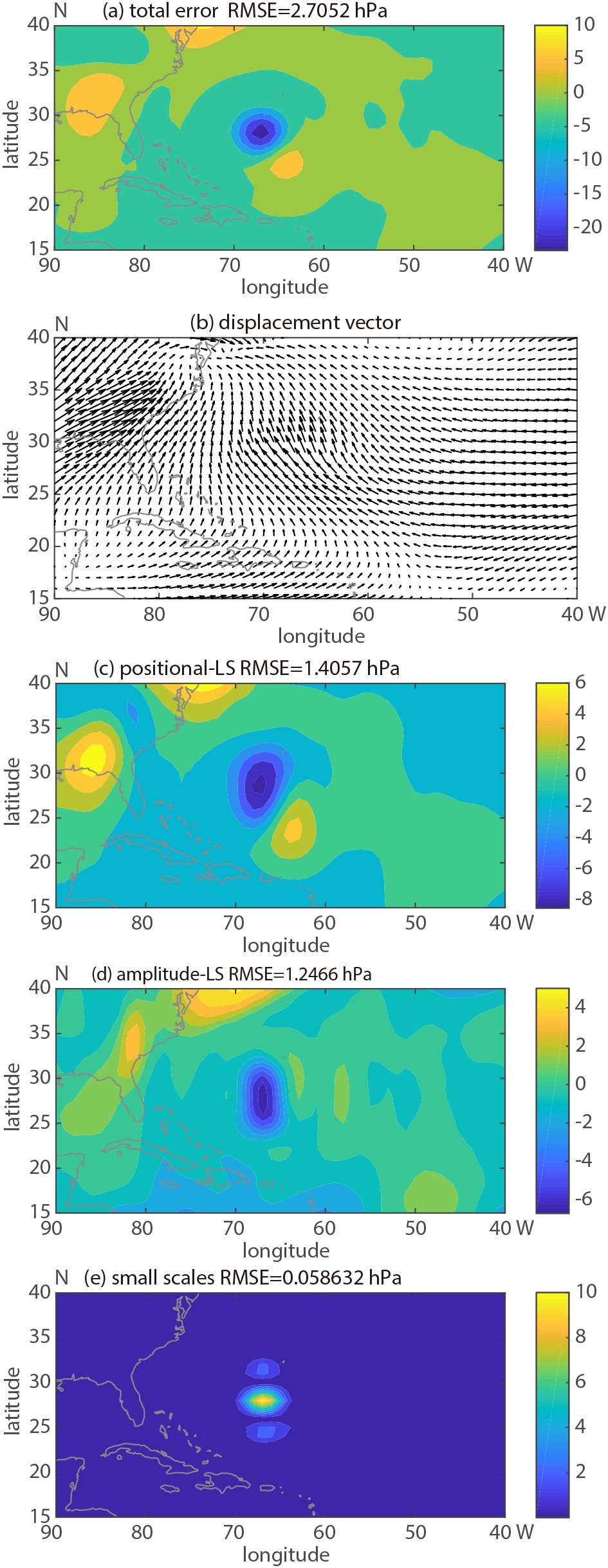Figure3. Total error (a), displacement vector (b), large scale positional error (c), large scale amplitude error (d) and small scale error for the 84 h lead time GEFS Control member MSLP forecast initialized at 0000 UTC on 3 September 2011. The domain average Root Mean Square Error/Difference (RMSE/RMSD) is included for panels a, c, d and e. Error Variance/difference magnitudes are illustrated with the color bar (hPa).


Focusing on the area of hurricane Katia (2011), the large scale positional error (Fig. 3c) manifests as a dipole pattern, indicating a slower than observed movement of the forecast storm. The large scale structural error (Fig. 3d), on the other hand, has a single minimum, pointing to a forecast storm less intense than observed. While the magnitudes of the large scale positional and structural error are similar, small scale error (Fig. 3e) has a much lower magnitude, except over the hurricane itself (see area average error variance numbers on error panels in Fig 3).
The partitioning of the MSLP forecast error variance components as a function of lead times for the same Katia (2011) forecast also has been examined (Fig. 4). Interestingly, the total error variance initially grows, and then reaches a minimum for 48 h lead time before increasing again. Large scale positional and amplitude components of error follow the same trend as the total error. Importantly, for all lead times large scale positional error variance represents about ~50% of total error while the amplitude (structural) component contributes with only ~15%. The small-scale error variance mainly remains constant with time.
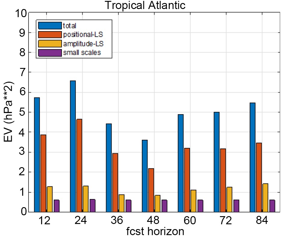Figure4. The error variance decomposition for MSLP, for different forecast horizons, calculated over the regional domain for a forecast initialized at 0000 UTC 6 September 2011.


Further inspection of the displacement vector field in Fig. 3b reveals a displacement over the southeastern US even larger than present around hurricane Katia (2011). This particular displacement in the MSLP forecast is associated with the position of frontal zones connecting multiple low pressure centers along the eastern US. To evaluate error partition related to this phenomenon and a different variable, a shorter lead time forecast (24 h) than was available for 850 hPa temperature was evaluated over a domain centered on the Eastern US. Figure 5 shows generally good agreement between the GFS analysis and the GEFS control (unperturbed) member 24 h forecast. More substantial differences between the analysis and GEFS control run appear over the Great Lakes area. The error decomposition is illustrated in Fig. 6. Higher values in large scale amplitude error component are detected over the Great Lake area (Fig. 6d). Similarly, the large-scale positional error component is characterized by similar features in addition to displaying greater amplitudes along the east US coast (Fig. 6c). The domain averaged RMSE values show larger contribution to the total error coming from the positional component (~61%) as compared to the amplitude component (~28%). Small scale error is confined over limited areas in the Great Lake region and along the frontal zone (Fig. 6e).
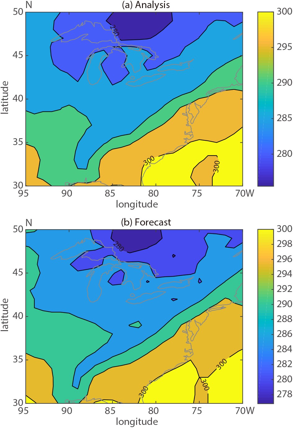Figure5. GEFS control member 24 h forecast and the GFS analysis valid at 1200 UTC 6 September 2011.


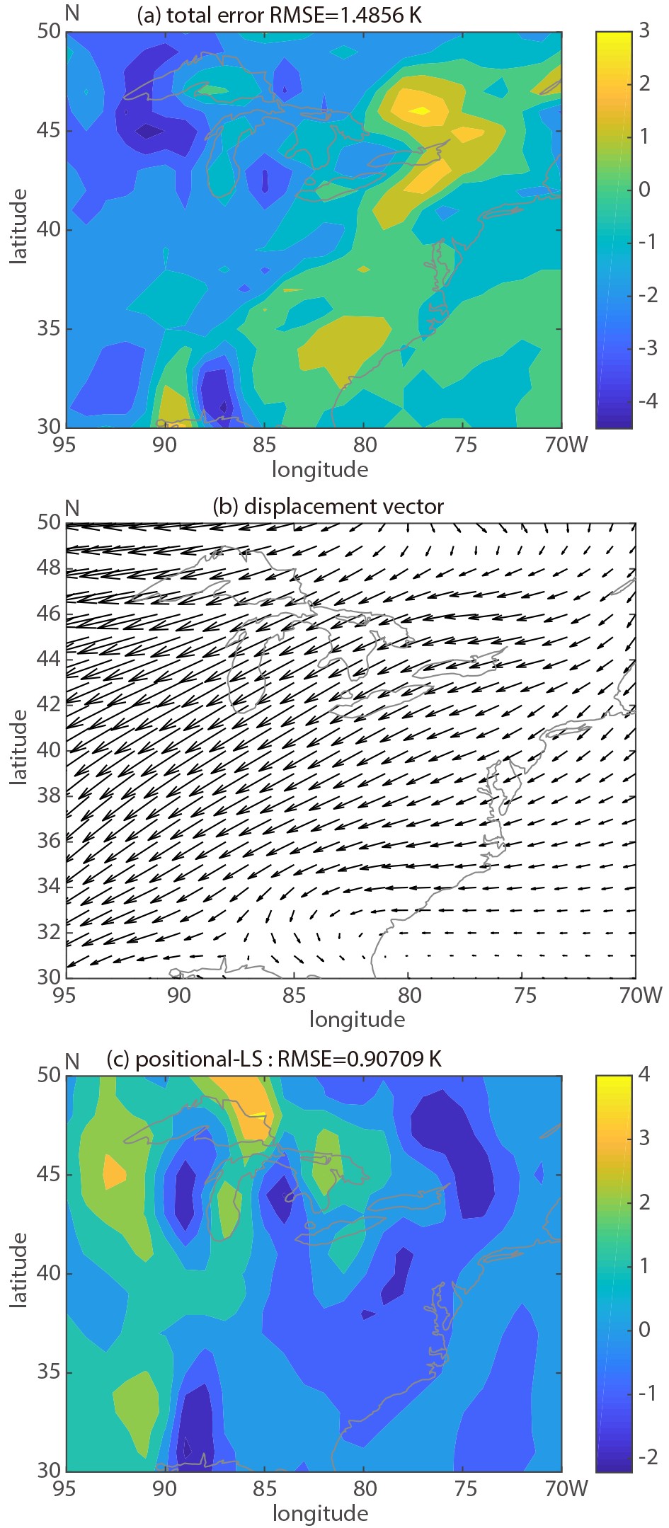Figure6. As in Fig. 3, except for 850 hPa temperature, 24 h lead time and the domain centered on Eastern US.


For a statistically more informative evaluation of FED results, Fig. 7 displays the magnitude of the three orthogonal error components over three large non-overlapping regions (tropics, Northern and Southern Hemisphere), averaged over the month of September 2011. First, we note that as expected, the total error (blue bars in Fig. 7) generally exhibits a growing tendency with increasing lead times. In all regions and at all lead times, large scale positional error (red bars) is the largest of the three components. Approximately 50%, 60%, and 75% of the total error variance is associated with the large-scale positional error for features over the Tropics, the Northern and Southern hemispheres, respectively. Large scale positional error in general also displays a growing tendency as a function of lead time, indicative of chaotic error growth.
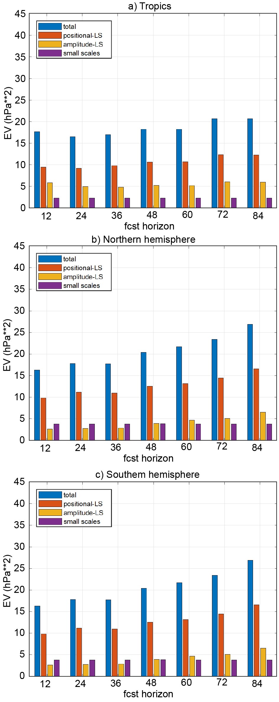Figure7. As in Figure 4, except for various regions of the globe (tropics—30°S?30°N, Northern—30°?90°N, and Southern hemispheres—30°?90°S) and for the entire month of September 2011.


Over the different lead times and domains, large scale structural and small scale error variance is ~20%?30% and ~10%?15% percent of the total error variance, respectively. In contrast to the large scale positional error, these error components do not always exhibit a growing tendency with increasing lead time. For example, large scale structural / small scale errors do not have a clear growing tendency over the Tropics / Tropics and NH, respectively. The lack of error growth in these regions may be indicative of model error in representing natural phenomena in these regions.

A Forecast Error Decomposition (FED) method has been proposed and demonstrated, partitioning the total forecast error into three orthogonal components: large scale positional, large scale structural, and small scale error. FED uses the Field Alignment (FA) technique of Ravela (Ravela, 2007) to align a forecast field with the verifying analysis field on a point-by-point basis to minimize their differences subject to a predefined smoothness constraint. Positional and structural errors are defined and orthogonalized in a low-pass filtered (“smooth”) subspace, ensuring that the filtered-out, high frequency error component also lies orthogonal to the large-scale components. To our knowledge, FED is the first attempt at such an orthogonal error decomposition. For example, the partitioning of Hoffman et al (1995) does not guarantee the orthogonality. While in the present study we fixed the value of the smoothness parameter, in future investigations, more smoothing can be applied at longer lead times, reflecting the increasing level of noise, and decreasing level of information at longer lead times.
The main focus of this study was to demonstrate the use of the FA technique in FED for quantifying major modes of forecast error. The use of FED was illustrated through a case study [Hurricane Katia (2011)] where the approach was applied to two different variables, MSLP and 850 hPa temperature (Figs. 3 and 6), and through MSLP error statistics calculated over a month-long period (Sep. 2011, Fig. 7). Both approaches showed consistent results. A significant portion of forecast error variance (~50%?70%, depending on geographical region and lead time) is associated with large-scale displacement of forecast features. Notably smaller portions of the total error variance are related to large-scale structural and small-scale error variance. The generality of these results will need to be assessed over extended datasets.
In certain applications, feature-based error decomposition techniques have been used extensively. Errors in TC forecasts, for example, have been described in terms of position and intensity errors. Such applications (a) require the identification of certain features (e.g., the center of a TC), and (b) limit the forecast evaluation to the pre-selected feature. In contrast, with its more general approach, FED offers more detailed, gridded information pertaining not only to pre-selected features but to their environment as well. In case of TC forecasts, for example, the quality of the forecasts can be described by displacement vector and structural error fields, instead of just the error in the position and intensity of the central (or another selected) point of the storm (cf. Fig 3).
Though FA has so far been demonstrated only on 2D fields, its extension to 3D is feasible. Even in its current form, the spatially distributed approach of FED naturally lends itself for use in more thorough diagnostic studies. Potential applications include the assessment of systematic errors in terms of positional and amplitude components. Detailed analyses of various experiments can provide useful feedback to model and data assimilation technique developers by suggesting areas that may be dominated more by positional or structural errors, associated more either with initial value (e.g., amplifying) or model related (e.g., systematic structural) uncertainties, respectively.
Forecasters have long expressed an interest in separately assessing uncertainty in the phase (i.e., position) and amplitude of forecast features (see, e.g., NCEP, 2004). Given the encouraging experiments reported here, we advocate for the more widespread use of gridded error decomposition tools such as that tested in the current paper.
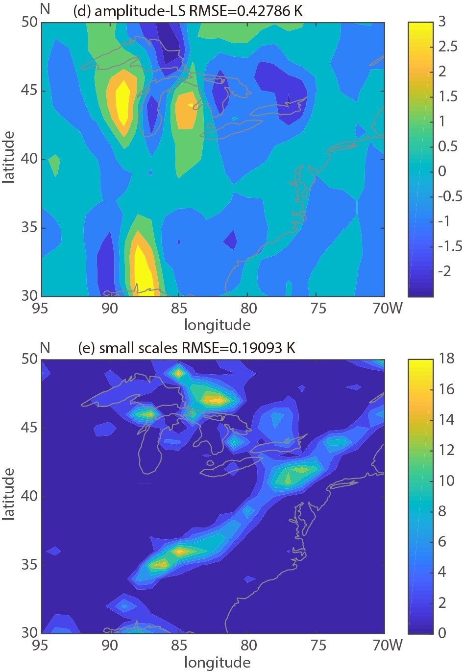Figure6. (Continued)


Acknowledgements. The authors would like to thank Tim MARCHOK of GFDL for helpful discussions, Dr. Michael BRENNAN of NHC for providing along and across track error statistics for Hurricane Katia (2011), and Drs. Jie FENG, Lidia TRAILOVIC, Edward TOLLERUD (all formerly affiliated with GSL), and two anonymous reviewers for their comments on an earlier version of this manuscript.