Jiawei YAO^1,2,
Wansuo DUAN^1,2,,,
Xiaohao QIN¹

Corresponding author: Wansuo DUAN,duanws@lasg.iap.ac.cn;

1.State Key Laboratory of Numerical Modeling for Atmospheric Sciences and Geophysical Fluid Dynamics (LASG), Institute of Atmospheric Physics, Chinese Academy of Sciences, Beijing 100029, China
2.University of Chinese Academy of Sciences, Beijing 100049, China
Manuscript received: 2020-03-18
Manuscript revised: 2020-11-17
Manuscript accepted: 2020-12-03
Abstract:Among all of the sources of tropical cyclone (TC) intensity forecast errors, the uncertainty of sea surface temperature (SST) has been shown to play a significant role. In the present study, we determine the SST forcing error that causes the largest simulation error of TC intensity during the entire simulation period by using the WRF model with time-dependent SST forcing. The SST forcing error is represented through the application of a nonlinear forcing singular vector (NFSV) structure. For the selected 12 TC cases, the NFSV-type SST forcing errors have a nearly coherent structure with positive (or negative) SST anomalies located along the track of TCs but are especially concentrated in a particular region. This particular region tends to occur during the specific period of the TCs life cycle when the TCs present relatively strong intensity, but are still intensifying just prior to the mature phase, especially within a TC state exhibiting a strong secondary circulation and very high inertial stability. The SST forcing errors located along the TC track during this time period are verified to have the strongest disturbing effect on TC intensity simulation. Physically, the strong inertial stability of TCs during this time period induces a strong response of the secondary circulation from diabatic heating errors induced by the SST forcing error. Consequently, this significantly influences the subsidence within the warm core in the eye region, which, in turn, leads to significant errors in TC intensity. This physical mechanism explains the formation of NSFV-type SST forcing errors. According to the sensitivity of the NFSV-type SST forcing errors, if one increases the density of SST observations along the TC track and assimilates them to the SST forcing field, the skill of TC intensity simulation generated by the WRF model could be greatly improved. However, this adjustment is most advantageous in improving simulation skill during the time period when TCs become strong but are still intensifying just prior to reaching full maturity. In light of this, the region along the TC track but in the time period of TC movement when the NFSV-type SST forcing errors occur may represent the sensitive area for targeting observation for SST forcing field associated with TC intensity simulation.
Keywords: tropical cyclone,
sea surface temperature,
sensitivity,
error growth,
inertial stability
摘要:热带气旋（TC）强度的模拟和预报仍有很大不确性，在导致TC强度模拟不确定性的所有误差来源中，海温误差有着重要作用。该研究利用WRF模式，采用非线性强迫奇异向量（NFSV）方法，揭示了对TC强度模拟不确定性影响最大的海温强迫误差，即NFSV型海温强迫误差。对于给定的12个TC个例，研究发现它们的NFSV型海温强迫误差均沿着TC路径分布，且具有几乎一致的特定空间结构，误差能量主要集中在某个特定区域。分析发现，该区域通常出现在TC快速增强且接近强度峰值的时间段，此时的TC尤其具有强次级环流和最高惯性稳定度的状态特征。从误差发展演变看，海温强迫误差首先引起潜热释放的误差，进而扰动次级环流，随后显著影响TC眼区的下沉气流，最后影响暖心强度，导致TC强度的不确定性。在TC快速增强接近成熟的时间段，TC所具有的最高惯性稳定度，使得次级环流对潜热释放误差有最强的响应，从而导致TC移动到该时间段时，其路径上的海温强迫误差能够最大限度地影响TC强度。该机制也使得对TC强度不确性影响最大的海温强迫误差主要集中在该时间段，从而解释了NFSV型海温强迫误差特殊结构形成的主要原因。根据NFSV型海温强迫误差呈现的敏感性可知，如果我们优先在TC增强接近成熟阶段的路径上加强海温观测，并将其同化到海温强迫场，TC强度的模拟水平会显著提高。所以，NFSV型海温强迫误差识别了TC强度模拟的海温目标观测的敏感时间段和敏感区域。
关键词:TC强度,
非线性强迫奇异向量,
可预报性,
海温强迫,

HTML

--> --> -->

A tropical cyclone (TC) is one of the most destructive synoptic scale systems on earth. It frequently brings great economic loss to coastal areas and even interior locations of countries (Peduzzi et al., 2012). It is therefore important to improve the skill of TC forecasts. With recent improvements of model simulation capability, to include data assimilation methods, great progress has been made resulting in greater skill regarding TC track forecasting. However, forecasting TC intensity still presents a huge challenge. The main reason for this is that TC intensity is not only dependent upon large-scale environmental factors such as vertical wind shear and sea surface temperature (SST) but also upon mesoscale/microscale processes represented by parameterizations such as moist convection, microphysics, etc. (Emanuel et al., 2004; Wang and Wu, 2004; Zhang et al., 2011; Hakim, 2013; Zhang and Tao, 2013; Tao and Zhang, 2014; Torn, 2016). The uncertainties of these factors operating at different spatial scales and their interactions with one another, complicate and therefore limit the predictability of TC intensity. Emanuel and Zhang (2016) used the Coupled Hurricane Intensity Prediction System (CHIPS; Emanuel et al., 2004) to explore the sources of TC intensity forecasting uncertainties. They found that the TC intensity errors grow during the early stages of development and is dominated by initial intensity errors, while the errors of TC track and environmental shear become more pronounced in affecting TC intensity during later developmental periods. Torn (2016) compared the role of atmospheric uncertainties and oceanic uncertainties in TC intensity simulation error and found that although the atmospheric uncertainties dominate during the initial period, oceanic uncertainties become equally as important during later periods. One may conclude that the inclusion of oceanic uncertainties can help to improve the predictability of TC intensity.
Previous studies reported the influence of SST on TC intensity either in theories or through observations. On one hand, the ocean is thought to be the energy source for TC genesis and intensification (Riehl, 1950; Emanuel, 1986, 1988; Holland, 1997). Specifically, the theory of maximum potential intensity (MPI), proposed by Emanuel (1986), treated TCs as heat engine. The MPI of TCs is a function of SST, outflow temperature and other relevant parameters, where the outflow temperature over tropical and subtropical oceans is strongly controlled by SST (Reid and Gage, 1981). In particular, the outflow temperature was shown to be linearly correlated to the SST, especially when the SST is higher than about 24 C but smaller than 29 C (DeMaria and Kaplan, 1994; Schade, 2000) [see Fig.1 in Schade (2000)]. Therefore, the MPI of TCs is almost exclusively determined by the SST. Moreover, the rate of TC intensification is also strongly affected by SST (?rnivec et al., 2016; Xu et al., 2016). Specifically, it is known that TCs absorb heat energy from the ocean and intensify due to the strong TC-ocean interaction which is potentially enhanced when TCs encounter warm oceanic eddies or rings (Lloyd and Vecchi, 2011; Yablonsky and Ginis, 2012; Kilic and Raible, 2013; Ma et al., 2017). The rapid intensification of both Hurricane Opal and Katrina, occurred when they moved through warm oceanic eddies. In the case of Katrina, it was the warm Loop Current of the Gulf of Mexico. (Hong et al., 2000; Shay et al., 2000; Scharroo et al., 2005). More specifically, Hong et al. (2000) demonstrated that a 1K SST increase will induce a drop in minimum central pressure of a TC by 10 hPa through a warm eddy sensitivity experiment. On the other hand, due to entrainment/mixing and upwelling processes, SST cooling always occurs along the right side of the track and can be as large as 4 K (Price, 1981; Schade and Emanuel, 1999; Schade, 2000; Davis et al., 2008). The cooler sea surface will inhibit the upward entropy flux and eventually reduce the intensity of TCs. Therefore, in order to improve the forecasting skill regarding TC intensity, a well-simulated SST forcing field is necessary. However, quite a lot of numerical models use a fixed SST forcing field and ignore the “SST cooling”, leading to an overestimation of the TC intensity (Winterbottom et al., 2012; Sun et al., 2014). Even if coupled models were used, the model errors of the atmospheric and oceanic components and its coupling frequency will reflect the error of a simulated SST (Davis et al., 2008; Strazzo et al., 2016; Scoccimarro et al., 2017). We may conclude that the SST error is inevitable. Therefore, it is necessary to estimate the potential effect of SST uncertainties upon TC intensity and then try to minimize this effect, ultimately improving the TC intensity forecast skill.
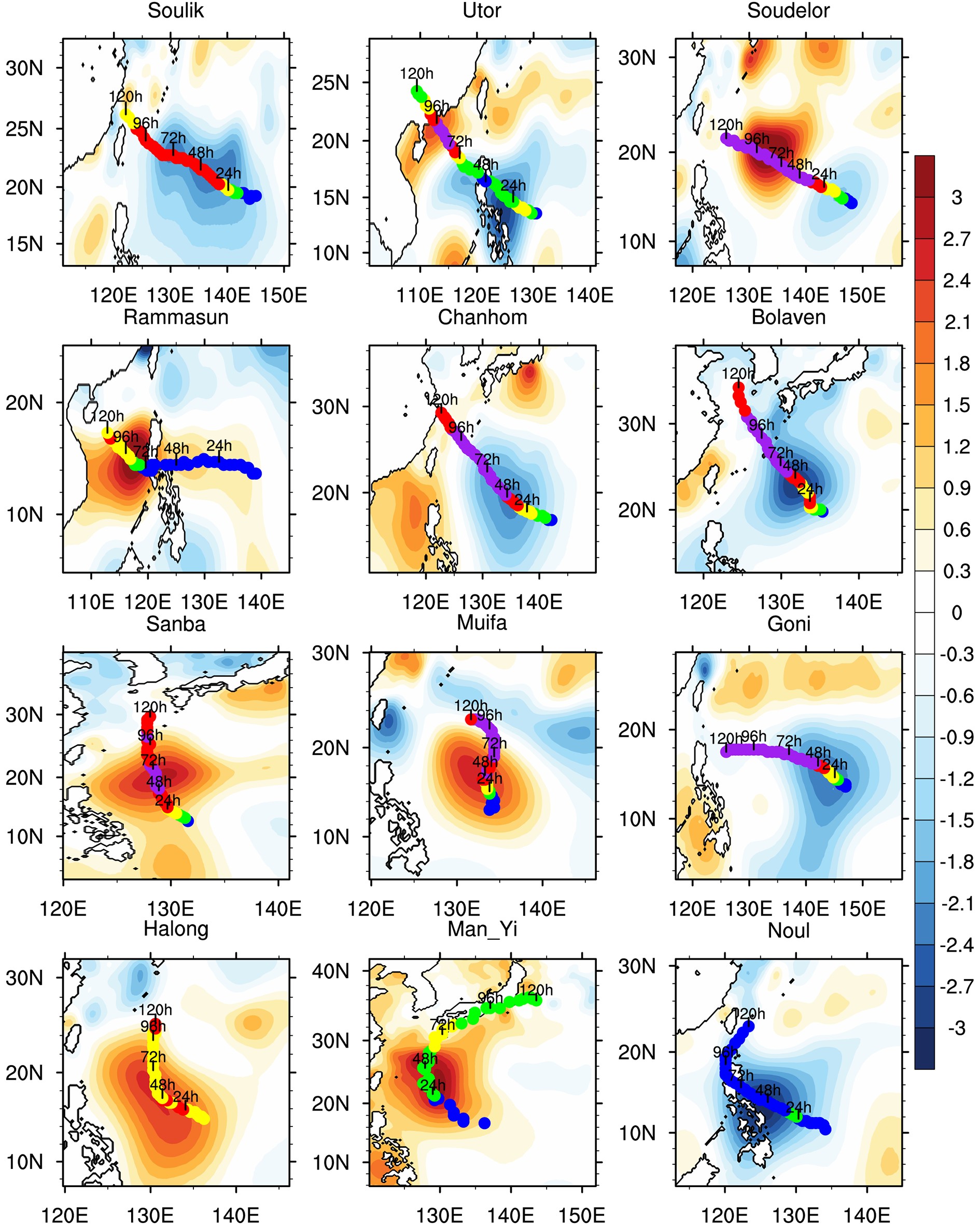Figure1. The patterns of the NFSV-type SST forcing errors (K) of the selected 12 TC cases. The blue, green, yellow, red and purple dots indicate the TC intensity of the unperturbed run within [980, 1000], [970, 980], [960, 970], [950, 960] and [900, 950] (hPa).


Most of operational TC forecasting models are composed of numerical weather forecasting models with a fixed SST forcing field, rather than applying an ocean-atmospheric coupled model, although the latter is of great expectation. Therefore, we analyze these weather forecasting models to explore the effect of the uncertainties of SST forcing on TC intensity simulation errors. To make the SST forcing more realistic, we adopt, in the present study, the observed time-dependent SST, rather than a fixed SST, as an external forcing of TC system and consider the effect of the errors superimposed on these SSTs upon the simulation of TC intensity, in attempt to explore which error has the largest effect on TC intensity. Here, the error of the SST forcing may describe the uncertainties occurring in SST due to inaccurate SST observations or imperfect TC-ocean interactions as indicated by a coupled model. Based on this analysis, we naturally ask how to improve the accuracy of the SST forcing or the TC-ocean interaction factors associated with TC intensity. It is certainly true that an increase in SST observations will improve the SST forcing field; while improvements regarding the TC-ocean interaction factors require improvements within a coupled model, which is also dependent upon having sufficient observations. Obviously, both of these aspects rely upon increasing observations. The question then is, in order to improve the result of TC intensity simulation efficiently, in which regions should the density of SST observations be increased?
The above question is related to a new observational strategy called “targeted observation” (Snyder, 1996; Mu, 2013). The tool of “targeted observation” was developed in the 1990s and originally proposed for an initial value-problem. Its general idea is as follows: to better predict an event at a future time t₁ (verification time) in a focused area (verification area), additional observations are deployed at a future time t₀ (targeted time, t₀ < t₁) in some special areas (sensitive areas) where additional observations are expected to contribute most profoundly to reducing the prediction errors in the verification area [Mu (2013)]. These additional observations can then be introduced into a model by a data assimilation system to form a more reliable initial state, which results in a more accurate prediction or simulation [see Fig. 1 in Majumdar (2016) for a schematic example for targeted observation].
Generally, targeted observation is used to decrease the initial error (Peterson et al., 2006; Buizza et al., 2007; Wu et al., 2007; Qin and Mu, 2012; Duan and Hu, 2015; Zou et al., 2016; Zhang et al., 2017). To deal with uncertainties of external forcing upon simulation skill, Wen and Duan (2019) extended the idea of targeted observation to treat the forcing error and considered which observations are more helpful for reducing forcing error and improving simulation skill. In the present study, TC simulation is investigated from the perspective of the SST forcing influencing TC intensity. Therefore, the targeted observation associated with reducing the forcing error proposed by Wen and Duan (2019) can be reasonably adopted to deal with the external forcing of SST observations for TC intensity simulation.
The key of targeted observation is to determine the sensitive area, defined here as the area where the simulation uncertainties are most sensitive to the forcing errors. In the present study, we would first identify the most sensitive SST forcing error and then subject the sensitive area to targeted observation associated with a TC intensity simulation. In order to identify the most sensitive error of the SST forcing, the approach of Nonlinear Forcing Singular Vector (NFSV) proposed by Duan and Zhou (2013) is useful. The NFSV represents the forcing error leading to the largest forecast/simulation error. The NFSV approach has been applied to the predictability studies of ENSO and Kuroshio Current effectively and succeeded in obtaining the most sensitive forcing error (Duan and Zhao, 2015; Wen and Duan, 2019). Through observation system simulation experiments (OSSEs), Wen and Duan (2019) showed that the region of large values in the NFSV-type errors represents the sensitive area for targeted observation associated with external forcing errors. In light of these successes, the present study uses the NFSV approach to determine the sensitive area for targeted observation associated with the TC intensity simulation. Thus, we seek answers to the following questions. 1) What kind of SST forcing error can lead to the largest TC intensity errors? 2) What kind of properties does the sensitivity of TC intensity on SST error have? 3) Does the structure of NFSV-type errors indicate the sensitivity of TC intensity on SST errors? 4) Which region, in time and space, represents the sensitive area for target observation for TC intensity simulation?
The arrangement of this paper is as follows: the settings of model, approach and algorithm is briefly introduced in section two. The NFSV-type SST forcing errors for 12 TC cases are calculated and corresponding sensitivity are shown in section three. In section four, the TC states responsible for the occurrence of the NFSV-type SST forcing errors are revealed and associated physical mechanisms are explored. In section five, the mechanism of the NFSV-type SST forcing error inhibiting TC intensity is discussed. Finally, a summary and a discussion are made in section six.

2

-->

2.1. Model

The regional model used in the present study is the Advanced Research Weather Research and Forecasting (WRF) model (ARW) in its version 3.8.1 (Skamarock et al., 2008). This particular version of the WRF model is fully compressible and based upon the non-hydrostatic Euler equations and has often been used in studies of TCs. The model adopts the microphysics scheme of Lin et al. (1983) and the Kain-Fritsch scheme for cumulus parameterization (Kain, 2004). The model considers the longwave and shortwave radiation by using the Rapid Radiative Transfer Model (RRTM; Mlawer et al., 1997) and the Dudhia scheme (Dudhia, 1989). The boundary layer is parameterized by the Yonsei University scheme (Hong et al., 2006).The TC simulation conducted by the WRF is subject to SST forcing that is updated every 6 hours; that is to say, TC is forced by a time-dependent SST field. The WRF here adopts the horizontal resolution of 30 km×30 km without nesting and 24 levels in the vertical direction. The model top is set as 5000 Pa and the time step of simulation is 90 s. All TC cases in the present study are simulated for 120 hours.
The atmospheric data (including variables associated with wind, pressure, cloud, soil, precipitation, etc.) adopted here is the FNL reanalysis from National Centers for Environmental Prediction (NCEP), whose resolution is 1×1 degree. The SST observation data is from NCEP and has resolution of 0.083×0.083 degree whose interpolated data is updated every six hours by the ungrib process, which assimilates in the SST data that is used to force the WRF model.

2 -->

2.2. Approach: Nonlinear Forcing Singular Vector

The Nonlinear Forcing Singular Vector (NFSV) was proposed by Duan and Zhou (2013), which is an extension of (linear) forcing singular vector (FSV; Barkmeijer et al., 2003) in nonlinear regime. For convenience, the NFSV is briefly described as follows.
Assume that the Eq. (1) describes a state equation
where G(U) and F(x,t) is model equation tendency and external forcing, and f(x) is a forcing error of the forcing term. According to the definition of NFSV, it is the tendency perturbation that generates the largest deviation from the reference state in a nonlinear model at a given time based on a physical constraint condition. For a given forcing error, the NFSV can be understood as the forcing error that has the largest effect upon the simulation or prediction error at the given future time. This can be formulated into the following optimization Eq. (2):
where J is cost function and the norms ||·||_a and ||·||_b measure the amplitude of the forcing error f and its resultant simulation error against the reference state, respectively. The forcing error, f, is subject to the constraint radius δ; M_t(f) and M_t(0) are the propagators of a nonlinear model with and without forcing error f(x) from time 0 to t, respectively; and U₀ is the initial value of the reference state. By solving Eq. (2), the NFSV, denoted by f* in Eq. (2) can be obtained.

2 -->

2.3. Algorithm: Particle swarm optimization

The particle swarm optimal (PSO) algorithm was initially proposed by Kennedy and Eberhart (1995) to imitate the process of bird foraging, but soon it was widely used to solve optimization problems and, in doing so, achieved great successes (Banks et al., 2008; Zheng et al., 2017). We will use this algorithm to calculate the optimization problem associated with NFSV. Next, we briefly describe the algorithm.
To make the cost function as in Eq. (2) to have the largest value in the given constraint condition, a series of particles characterized by positions (denoted by X; the forcing perturbations here) and velocities (denoted by V; the iteration velocity) are randomly generated. Then the cost function is calculated with these particles. These particles will be updated by iterations according to the values of the cost function. Specifically, the iterations are realized by calculating the Eqs. (3) and (4).
where k is the kth iteration step, m represents the mth particle, ${{P}}_m^k $ is the optimal position of the mth particle (which makes the cost function reach the largest for the former m particles) and ${{P}}_g^k $ is the optimal position of all particles after k iterations, ω is a weight, c₁ and c₂ are the acceleration coefficients, and s₁ and s₂ are two random numbers that are subject to a uniform distribution over the interval [0, 1]. If the cost function satisfies a criterion, the iterations can stop. Assume $J_m^k $ is the cost function of the mth particle after k iterations, and the number of the particles at the kth iteration is M. Then the algorithm obtains M values of the cost function at kth iteration step, i.e. ($J_1^k $, $J_2^k $, …, $J_M^k $). From these values, one can find the largest value $J_i^k $, then the corresponding ith particle position is the optimal particle position at kth iteration step. If the optimal particle position at the following iteration steps is unchanged, the iterations can stop and the NFSV just is the ith particle position, i.e. X.
For a high-dimensional dynamic system, it is impossible to generate particles with the same number as the dimensions of the model dynamical system to calculate the NSFV by using the PSO algorithm. Thus, we apply an empirical orthogonal function (EOF) analysis to reduce the dimensions and obtain the representative particles required by the PSO. For the SST forcing errors associated with TC intensity, we adopt the following strategy to generate the particles of the PSO algorithm.
(i) We take the SST field in the north-west Pacific region (i.e. 10o?35oN, 100o?150oE) every five days from 1 July to 30 September or from 1 June to 31 August during 2006?16. Which period is selected depends upon the season when TCs happen most frequently during the year. Then, we subtract the SST field on 1 July from that on 5 July (or on 1 June from that on 5 June). This method is also applied to the SST fields on 5 July from that on 10 July (or on 5 June from that on 10 June), on 10 July from that on 15 July (or on 10 June from that on 15 June), and so on. Then 198 SST forcing perturbations are obtained.
(ii) An EOF analysis is applied to the 198 SST forcing perturbations and the leading 30 dominant modes are experimentally selected to yield the NFSV. The 30 dominant modes explain 80% of total variance of SST forcing perturbations which is believed to be enough for searching the NFSV using the PSO algorithm.
(iii) We scale the leading 30 modes to have the same amplitude in terms of the adopted norm (see next section) and assign them as the initial positions of particles, while the initial velocities of particles are, at first, guessed as being equal to their initial positions.

In the present study, 12 TC cases are selected according to the best-track data from the Japan Meteorology Agency (JMA) for exploring the sensitivity of TC intensities on the SST forcing errors. The 12 TC cases are chosen according to the following criteria: (1) the TCs which greatly influenced China, (2) the lifetimes of TCs were longer than 5 days and stayed over the ocean during the overwhelming majority of the simulation period, and (3) the TC whose tracks were minimally altered when the SST forcing was modified, with the largest deviation of this subset being less than 60 km when the SST forcing is modified, which almost excludes the impacts of the bias of TC tracks on TC intensities. The brief information concerning the selected 12 TCs is listed in Table 1. The geometric centers of the TCs are identified as the locations with the minimum sea level pressures (MSLPs), which are utilized to represent the TC intensities hereafter. The NFSV represents a special type of SST forcing error, with which the simulated TC intensities depart the most from, as compared to without it, as Eq (5) describes.

Name	No.	Start time (h; UTC)	End time (h; UTC)	Time of TC mature phase (h; UTC)	TC intensity at mature phase
Soulik	201307	0000 Jul 08	0000 Jul 13	0000 Jul 10	925 hPa; 50 m s?1
Utor	201311	0000 Aug 10	0000 Aug 15	1200 Aug 11	925 hPa;53 m s?1
Soudelor	201513	0000 Aug 02	0000 Aug 07	1800Aug 03	900 hPa;57 m s?1
Rammasun	201409	0000 Jul 13	0000 Jul 18	0600 Jul 18	935 hPa; 45 m s?1
Chanhom	201509	0000 Jul 06	0000 Jul 11	1800 Jul 09	935 hPa; 45 m s?1
Muifa	201109	0000 Jul 29	0000 Aug 03	1800 Jul 30	930 hPa; 48 m s?1
Bolaven	201215	0000 Aug 23	0000 Aug 28	1200 Aug 25	910 hPa; 50 m s?1
Sanba	201216	0000 Sep 12	0000 Sep 17	1800 Sep 13	900 hPa; 55 m s?1
Goni	201515	0000 Aug 15	0000 Aug 20	0600 Aug 17	935 hPa; 48 m s?1
Halong	201411	0000 Aug 02	0000 Aug 07	1200 Aug 02	920 hPa; 53 m s?1
Man-Yi	200704	0000 Jul 11	0000 Jul 16	1200 Jul 12	930 hPa; 48 m s?1
Noul	201506	0000 May 07	0000 May 12	0000 May 10	920 hPa; 55 m s?1
Note: The numbers (No.) and intensities are from the best-track data of JMA (Japan Meteorological Agency), the latter of which include the minimum sea level pressure and maximum surface wind speed at the corresponding time.

Table1. Twelve TC cases of investigation


Here, T represents the SST that forces the WRF model during the simulation period and updates every 6 hrs. δT denotes the SST forcing error that is superimposed to T. $\left\| {\delta {{T}}} \right\| \leqslant 1$, where $\left\| {\delta {{T}}} \right\| = \sqrt {\displaystyle\sum {\delta {{{T}}^2}(i,j)/N} } $ constrains the standard deviation of superimposed SST forcing errors not larger than 1 K, which is determined by the mean anomaly of SST in the western North Pacific region [i.e. 10o?35oN, 100o?150oE; (i, j) is the grid point in this region] 5 days before and after a storm passes, $P({{T}},t)$ and $P({{T}} + \delta {{T}},t)$ represent the MSLP at time t without and with the forcing error δT, respectively. For simplicity, we refer to the former as an unperturbed run and the latter as a perturbed run. For each TC case, the MSLPs are calculated at 3 hrs intervals during the 120 hrs (i.e. 5 days) simulation. Thus, there are 41 MSLPs calculations in each run. The cost function J represents the sum of the deviations of these MSLPs in the perturbed run from those in the unperturbed run measured by absolute values, which indicates the total error of the TC intensity simulation during the 120 hrs. Here, the PSO algorithm is utilized to solve Eq. (5) and the NFSV ($\delta {{T}}^*$) denotes the SST forcing error that has the largest effect upon TC intensity, which is referred to as NFSV-type SST forcing errors hereafter for simplicity.
The NFSV-type SST forcing errors are calculated for the predetermined 12 TC cases and plotted in Fig. 1. It is shown that, although the tracks of these 12 TC cases differ a lot from each other, the NFSV-type SST forcing errors are always along the TC tracks. This indicates that the SST errors in the areas along the TC tracks, compared with those in the areas away from the TCs, are likely to exert a greater influence the TC intensities. Although the NFSV-type SST forcing errors are located along the TC tracks, they display the largest anomalies in different time periods (e.g. from 24 h to 48 h for Soulik, from 60 h to 96 h for Rammasun, and so on; see Fig. 1) of the different TCs. Recalling the definition of the aforementioned NFSV scheme, the NFSV-type SST forcing errors represent the forcing errors that result in the largest TC intensity simulation errors over the 120 hrs. Then the distribution of the NFSV-type SST forcing error along the TC track may indicate that the TC intensity simulations that are significantly sensitive to the SST forcing errors occurring in a particular time period of TC movement.
To clarify the above sensitivity of the NFSV-type SST forcing errors, we propose the following experiment. It is known that the ensemble spread is often used to measure the sensitivity. As such, we select 22 SST forcing perturbations randomly from the predetermined 198 perturbations (see section 2.3) to form an ensemble and scaled them to have an amplitude of 1 K, measured by $\left\| {\delta {{T}}} \right\| = $$ \sqrt {\displaystyle\sum {\delta {{{T}}^2}(i,j)/N} } $ [see Eq. (5)], which is the same amplitude as in the NFSV-type forcing errors, for evaluating the sensitivity. Interestingly, when we selected more SST forcing perturbations in this experiment, the result did not change. Therefore, we just use these pre-determined 22 SST forcing perturbations to describe the result. The 22 SST forcing perturbations are superimposed upon the unperturbed SST forcing fields (used in the unperturbed run) for TCs during the period of [t₀, t₀+6], with t₀ being 0 h, 6 h, 12 h, ..., 114 h and t₀+6 indicating the period lengthy being 6 hours, respectively. For each t₀, after the WRF model is integrated with the unperturbed SST forcing from 0 h to t₀ h, the 22 SST forcing perturbations are then superimposed during the interval, [t₀, t₀+6]. Then, the differences of the TC intensities between the unperturbed run and 22 perturbed runs during the interval, [t₀, t₀+6] are obtained. The ensemble spread of the 22 perturbed runs in the TC intensity represents the sensitivity of the TC intensity during the interval, [t₀, t₀+6] for the 22 SST forcing perturbations. With a changing t₀, it is conceivable that the ensemble spread in each 6 hrs can reveal the period of the TC movement, or evolution, that exhibits the strongest sensitivity of TC intensity to the 22 SST forcing perturbations. The spreads in each 6 hrs of all 12 TCs are plotted in Fig. 2. Clearly, the largest spreads occur in different time periods for different TCs. This indicates that the sensitivity of TC intensity to the SST forcing perturbations is dependent on the TCs themselves. Nevertheless, it is found that such sensitivity dependence upon TCs fits the distribution of the NFSV-type SST forcing errors well along the TC track (see Fig. 3). The details are as follows.
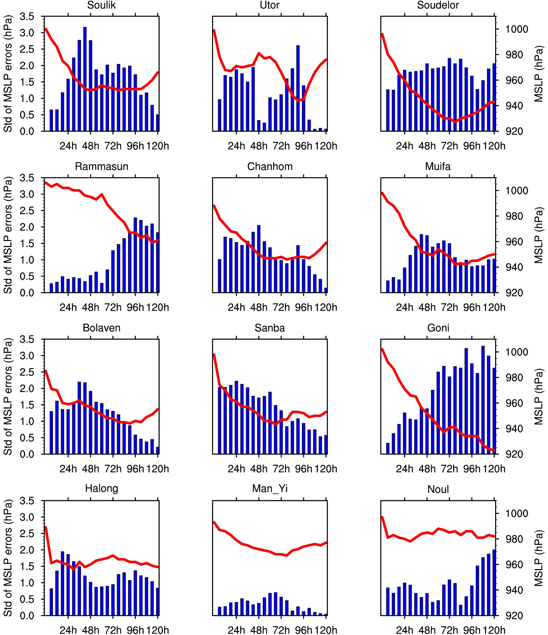Figure2. The spread of TC intensity simulations perturbed by 22 SST forcing perturbations during [t₀, t₀+6] with t₀ being 0 h, 6 h, 12 h, ..., 114 h and the TC intensity of the unperturbed run. Red lines denote the TC intensity [indicated by minimum sea level pressure (MSLP); units: hPa] of the unperturbed run. The blue bars represent the spread of the 22 perturbed runs of the TCs during [t₀, t₀+6] (units: hPa).


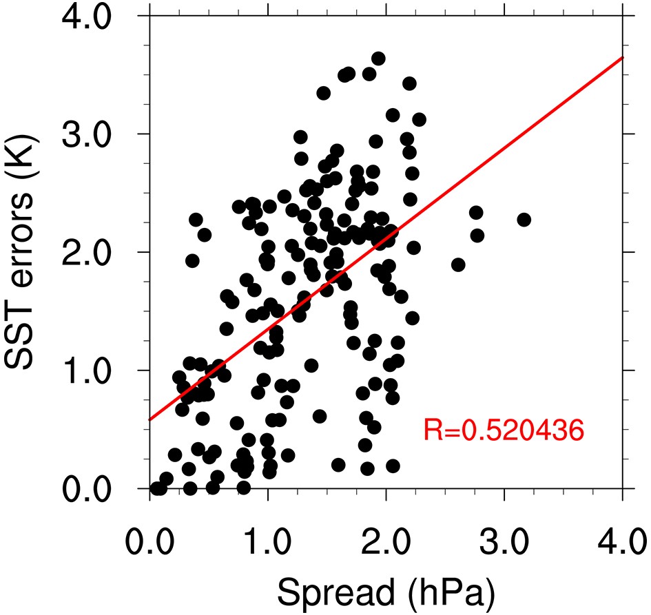Figure3. The regionally-averaged NFSV-type SST forcing errors at t₀ as a function of the spreads of TC intensity simulations perturbed by the 22 SST forcing perturbations during [t₀, t₀+6] with t₀ being 0 h, 6 h, 12 h, ..., 114 h. The red line represents the linear regression line between NFSV-type SST forcing errors and spreads.


The regionally-averaged NFSV-type SST errors of the selected 12 TCs, within a radius of 300 km, centered at the central location of the TC, and at t₀ are respectively calculated, which is plotted in Fig. 3 as a function of the spread of the 22 perturbed runs in TC intensity for each TC during the interval, [t₀, t₀+6]. With the change of t₀, the linear regression between the regionally-averaged NFSV-type SST forcing errors and the ensemble spread is calculated (see the line in Fig. 3). It follows that the regionally-averaged NFSV-type SST forcing errors are significantly correlated with the spread of the intensity in the perturbed runs of the TCs, which demonstrates significance at the 0.01 level when subjected to a t-test. That is to say, the larger the ensemble spread during one time period of TC, the larger the corresponding NFSV-type SST forcing errors. It is therefore obvious that the NFSV-type SST forcing errors can identify the time period when the TC intensity simulations are highly sensitive to the SST forcing errors.
The 22 randomly-selected SST forcing perturbations described above are further-superimposed on the unperturbed SST fields to force the TCs for the whole simulation period of 120 hrs. Then the total error of the TC intensity in each perturbed run, during the 120 hrs, is calculated for each TC. After this is done, the correlation coefficients are calculated at each grid point, for each TC between the total errors of the TC intensities in the perturbed runs and the corresponding member of the 22 SST forcing perturbations (see Fig. 4). Figure 1 shows that the distributions of the correlation coefficients are very similar to those of the corresponding NFSV-type SST errors. More specifically, the spatial correlation coefficients between them can be as large as 0.64, on average, for the 12 TC cases (the details can be seen in Table 2), indicating that the larger the ensemble spread particular to a TC location, the larger the NFSV-type errors there. It can also be seen that the correlation coefficients are much larger along the TC track, which implies that the total error of the TC intensity is especially sensitive to the SST forcing errors along the TC track. The similarity between the distributions of the correlation coefficients and the corresponding NFSV-type SST errors indicates that the NFSV-type SST errors link the sensitivity of the TC intensity simulation errors to the SST forcing errors in space. Furthermore, this relationship confirms that the SST errors in the areas along the TC tracks, especially those during the time period when the NFSV-type SST forcing errors attain large values, may significantly influence the TC intensities.
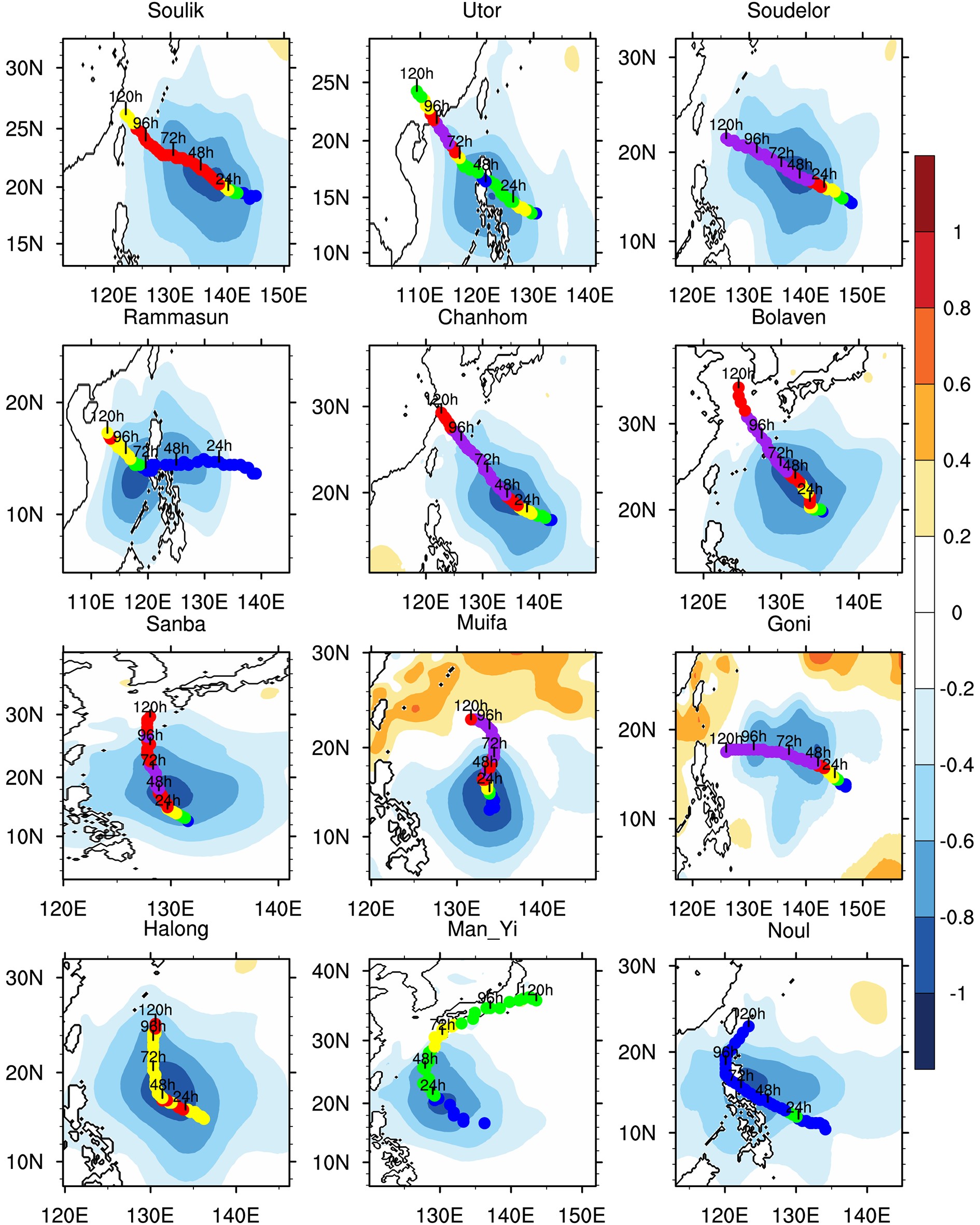Figure4. The spatial correlation coefficients (shaded) between the 22 SST forcing perturbations and the sum of the absolute values of intensity errors during the whole simulation period of 120 hrs for the selected 12 TC cases. The blue, green, yellow, red and purple dots represent the simulated TC intensity within [980, 1000], [970, 980], [960, 970], [950, 960] and [900, 950] (hPa).

	Cases
	Soulik	Utor	Soudelor	Rammasun	Chanhom	Bolaven	Sanba	Muifa	Goni	Halong	ManYi	Noul
Cor.	0.82	0.48	0.41	0.58	0.82	0.55	0.64	0.60	0.59	0.78	0.72	0.72

Table2. The spatial correlation coefficient between intensity errors and the 198 SST perturbations for 12 TC cases.

It is clear now that the NFSV-type SST forcing errors can identify the particular time period of the TC movement when the TC intensities exhibit high sensitivity to the SST forcing errors; but such time periods are dependent on the individual TC cases. The issue then becomes, whether or not these different time periods for different TCs correspond to common physical and environmental states of TCs. That is to say, what physical and environmental factors determine the sensitivity displayed by the NFSV-type SST forcing errors? Since the NFSV-type SST forcing errors cause the largest simulation errors of the TC intensity, we choose to explore the contributing factors of the NFSV-type SST errors by addressing which states of TCs are favorable for the SST forcing errors that yield large TC intensity errors. We go on to explain the physical processes responsible for the TC state that is consistent with the formation of the NFSV-type SST forcing errors.

2

-->

4.1. Which states of the TCs are favorable for the SST forcing error causing large intensity error?

We classify the lifetimes of TC movement into two categories of time periods according to the sensitivities of the simulated TC intensities in perturbed runs to the SST forcing perturbations. Specifically, for the selected 22 SST forcing perturbations and the time periods [t₀, t₀+6] as in section 3, if a time period possesses a spread (among the 22 perturbed runs in TC intensities) greater than 1.5 hPa (i.e. the mean value of the ensemble spreads during [t₀, t₀+6] with the changing t₀), this time period is categorized as a relatively high sensitivity period (referred to as “H-Sen” hereafter); conversely, the other time periods are categorized as relatively low sensitivity periods (referred to as “L-Sen” hereafter).
For the environmental factors, the SST, relative humidity (RH), vertical wind shear (VWS), and translation speed are considered. During the period [t₀, t₀+6] (noting that t₀ changes), all of the above environmental factors are calculated at t₀, t₀+3 hrs, and t₀+6 hrs for the unperturbed run, respectively. At each of these timings, the SST is regionally-averaged in a circular domain with a radius of 300 km centered at the simulated TC center; it is then further averaged consistent with the three timings. This averaged SST represents the environmental SST of the TCs in the period [t₀, t₀+6]. The VWS is similarly calculated, but denotes the difference of the regionally-averaged horizontal wind between 200 hPa and 850 hPa; and the RH is vertically averaged in the layers between 1 km and 6 km in the aforementioned circular domain. The translation speed, is calculated by taking the difference of the centers of the TC at both t₀ and t₀+6 hrs and then dividing this distance by the 6 hrs time interval. All of the above calculations are classified according to H-Sen and L-Sen and the results are shown in Table 3. It is found that the TCs in the H-Sen periods, compared with those in the L-Sen periods, have much more humid inner-cores, move profoundly slower over warmer SSTs, and are accompanied by stronger VWS. In previous studies, all of these environmental factors were shown to benefit the intensification of TCs (Mei et al., 2012; Zhang and Tao, 2013; Tao and Zhang, 2014; Walker et al., 2014; Torn, 2016; Zhao and Chan, 2017). Nevertheless, when we calculate the correlation coefficients between the spread of the 22 perturbed runs in TC intensity during the period [t₀, t₀+6], with the changing t₀, and the environmental factors of SST, RH, VWS, and translation speed in the unperturbed run, they are shown to be very low and thus weakly correlated [see Fig. 5 (a?d)]. This suggests that the environmental factors of TCs cannot be responsible for the relatively high sensitivity in the H-Sen period of TCs.

	SST	RH	VWS	Speed	MSLP	W	Vr	I2
H-Sen	302.0	66.0	8.10	19.82	957.9	0.26	?5.9	0.0042
L-Sen	301.2	53.0	6.50	26.42	965.9	0.17	?4.2	0.0029
P-value	0.0005	0.02	0.0104	0.0007	0.0016	1.8×10?6	2.1×10?5	1.1×10?5
Note: MSLP represents minimum sea level pressure (units: hPa) of the TCs; W, Vr, and I2 denotes corresponding vertical velocity (units: m s?1), radial velocity (units: m s?1), and inertial stability (units: s?2), respectively; and SST, VWS, Speed, and RH represents the absolute value of sea surface temperature (units: K), vertical wind shear (units: m s?1), translation speed of TC (units: m s?1), and the relative humidity (%). P-value indicates the significance level of the differences between the values in H-Sen and those in L-Sen.

Table3. TC states and their environmental factors during H-Sen and L-Sen


Figure5. The scatter plots between spreads of TC intensity simulation yielded by the 22 SST forcing perturbations and corresponding (a) SST forcing (units: K), (b) RH (units: %), (c) translation speed (units: km h^?1), (d) VWS (units: m s^?1), (e) vertical velocity (units: m s^?1), (f) inflow (units: m s^?1), (g) inertial stability (units: 10^?3 s^?2) and (h) MSLP (units: hPa). The red lines represent the linear regression. The red dots are for the H-Sen period and the black dots are for the L-Sen periods. The SST, RH, translation speed, VWS, vertical velocity, inflow, inertial stability and MSLP are calculated as in Table 3 (see section 4).


The characteristics of the TCs themselves in the H-Sen and L-Sen periods are also examined and associated inflow, vertical velocity, and inertial stability influencing TC intensity are calculated, respectively. Specifically, the inflow is calculated by taking the regionally-averaged radial component of the horizontal wind in a circular area centered at the simulated TC center, with the radii between 50 km and 300 km and vertically-averaged from 0 km to 1 km; the vertical velocity is estimated by a similar scheme but estimates the vertical wind by taking the vertically- and regionally-averaged component from 0 km to 15 km within a circular area centered at the simulated TC center with the radii between 50 km and 150 km; and the inertial stability is calculated by the formula ${I^2} = (f_c^{} + \xi)({f_c} + 2v/r)$ (where f_c is the Coriolis parameter, $ v $ represents the tangential wind velocity, $\xi $ denotes the relative vorticity, and $ r $ is the radius), which is then vertically and regionally-averaged from 0 km to 15 km and in a circular area, centered at the simulated TC center, with a radius of 100 km. The above results are also listed in Table 3 according to H-Sen and L-Sen. It is shown that the TC intensity in the H-Sen period is about 957.9 hPa on average, which is stronger than the average of 965.9 hPa in the L-Sen, and is found to be significant at the 0.0016 level using a t-test. This indicates that the TC intensities show higher sensitivity to the SST forcing errors when they are much stronger. We also note similar results from Table 3 with respect to the inflow, vertical velocity, and inertial stability; that is, these variables are much larger in H-Sen period, which is consistent with the presence of relatively strong TCs in the H-Sen periods. Furthermore, we calculate the correlation coefficients between the spread of the 22 perturbed runs in TC intensity during the period [t₀, t₀+6] with the changing t₀ and corresponding inflow, vertical velocity, inertial stability, and MSLP of the unperturbed run. We find that they, compared to those for the environmental factors, are more significantly correlated. This indicates that the TC intensities are much more sensitive to the SST forcing perturbations when the TCs exhibit strong intensity, larger inflow, large vertical velocity, and strong inertial stability (see Fig. 5). Moreover, from Fig. 2, it is shown that the TC cases tend to have the largest forecast spread when the TCs exhibit relatively strong intensity but are still intensifying, just prior to being fully mature, with the notable exception of TC Noul. To facilitate the discussion, such spatio-temporal period is hereafter called the Critical Time and Phase (CTP).
When we further examine the corresponding secondary circulation and inertial stability, it is found that the CTP period shows strong secondary circulation but the highest inertial stability for TCs. As an example, Fig. 6 plots the evolution of inertial stability, inflow, and vertical velocity of the TC Soulik (201307). It is shown that the inertial stability and the vertical velocity reach the largest values during the time period from 24 h to 48 h, while the inflow is still increasing in this period. Here, the time period from 24 h to 48 h fits the CTP of TC Soulik (also see Fig. 2). Therefore, we conclude that the strongest sensitivity of TC intensities to SST forcing perturbations occurs during the CTP of the TCs, especially with a TC state of the highest inertial stability and the strong secondary circulation. Such time periods can also be seen in Fig. 1, i.e. the period with the deepest color in the shaded area, during which the SST errors associated with the NFSV are of the largest assigned values. Particularly, the time period with the deepest color in the shaded area for the TC Soulik is about from 24 h to 48 h, which coincides with the CTP of the TC Soulik Therefore, the NFSV-type SST forcing errors locating at the TC track not only describe the sensitivity of the TC intensities to the SST forcing errors (see section 3) but also capture the time period of the TC movement when the TC intensity presents the strongest sensitivity to the SST forcing errors. Based upon these results, we advance the hypothesis that the TC states of high inertial stability and the strong secondary circulation are responsible for the NFSV-type SST forcing errors being dominated by the errors occurring during the CTP.
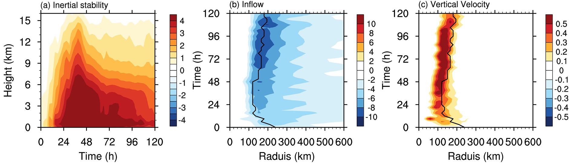Figure6. The evolution of (a) inertial stability (units: 10^?3 s^?2), (b) inflow (units: m s^?1) and (c) vertical velocity (units: m s^?1) for the TC Soulik. The inertial stability is regionally-averaged in a round area centered at the simulated TC center within 50 km; the inflow is an azimuthal mean of radial velocity, which is vertically-averaged in the layers between 0 km and 1.5 km; and the vertical velocity is vertically-averaged in the layers between 3 km to 7.5 km. The black lines in (b) and (c) denote the RMW at 2.0 km.



2 -->

4.2. Why do the SST forcing errors in the H-Sen period influence the TC intensity more significantly?

The eleven TC cases with the strongest sensitivity in their respective CTP are used to address the nature of the physical mechanisms which explain the enhanced sensitivity. To facilitate the discussion, we take TC Soulik as an example. It has been previously mentioned that the distribution of the NFSV-type SST forcing errors reflects the sensitivity of TC intensities to the SST forcing errors; and the NFSV-type SST forcing errors tend to have the largest anomalies during the time period from 24 h to 48 h of TC movement when the TC is during the CTP (see the NFSV-type SST forcing error pattern for the TC Soulik in Fig. 1). This time period is coincident with the strongest sensitivity of TC intensity on the SST forcing errors and is particularly associated with a strong secondary circulation and very highest inertial stability of the unperturbed run. The issue of concern is whether or not the along-track SST forcing errors that occurred during this unique and relative stage and timing in TC evolution, significantly differ from the response of TCs that exist at another timings in the TC growth cycle.
To address this concern, we conduct another group of experiments for intensity simulations of TC Soulik. We superimpose an artificial SST forcing error to the unperturbed SST forcing field at each grid point, where the SST error at each grid point is of uniform magnitude of ?1.0 K, which has the same amplitude as in the NFSV-type SST forcing errors calculated by $\left\| {\delta {{T}}} \right\| = \sqrt {\displaystyle\sum {\delta {{{T}}^2}(i,j)/N} } $ [see Eq. (5)]. We integrate the WRF for 120 hrs and obtain a perturbed simulation of the intensity of TC Soulik, hereafter as “UN-all” simulation. In addition, we also superimpose the above SST forcing error only during the H-Sen period of the TC Soulik (exactly, as its identified from 24 h to 96 h by the criterion determining the H-Sen; see section 4.1 and hereafter as “UN-Sen”) and then, only during the L-Sen periods (i.e. the period from 0 h to 24 h and from 96 h to 120 h; hereafter as “UN-non-Sen”), respectively. In this way, we may obtain two additional perturbed runs of the TC Soulik intensity forecast. Comparison is then made among these three perturbed runs to determine whether or not the SST forcing errors in H-Sen period causes a significantly larger intensity error compared to that in L-Sen period.
The errors of the TC intensities in the experiments of UN-all, UN-Sen, and UN-non-Sen with respect to the unperturbed run are shown in Fig. 7a. It can be seen that the error of the TC intensity in the UN-Sen experiment is significantly larger than that in the UN-non-Sen experiments and accounts for a forecast error of almost 80% compared to that in the UN-all experiment (Fig. 7b). This indicates that the total error of TC intensity in the UN-all experiment is mainly caused by the SST forcing errors during the H-Sen period. In addition, we can notice from Fig. 7a that the growth rate of the TC intensity error in the UN-Sen experiment is much larger than that in the UN-non-Sen experiment. Specifically, during the time periods from 0 h to 24 h and from 96 h to 120 h of the L-Sen periods in the UN-non-Sen experiment, the intensity errors are constrained to be than 6 hPa; while in the UN-Sen experiment, the intensity errors increase by about 10 hPa during the time period from 24 h to 48 h of the H-Sen period, which is the equivalent time interval of 24 hrs as the former two periods(from 0 h to 24 h and from 96 h to 120 h, in the L-Sen period). Furthermore, the time period from 24 h to 48 h of the H-Sen period coincides with the interval when the NFSV-type SST forcing error of the TC Soulik achieves the largest values and the TC intensities are most sensitive to the SST forcing perturbations. The rapid increase of the intensity error during the time period from 24 h to 48 h can also be seen in the UN-all experiment if one uses the slope of the error evolutionary curve to measure the error growth (see Fig. 7a). In particular, the time period from 24 h to 48 h shows the fastest growth of intensity error for the TC Soulik in the UN-all experiment, therefore, contributing the most to the total error of the TC intensity during the entire simulation period. This may explain why the NFSV-type SST forcing errors occur in the H-Sen period, particularly during the time period from 24 h to 48 h in the case of TC Soulik.
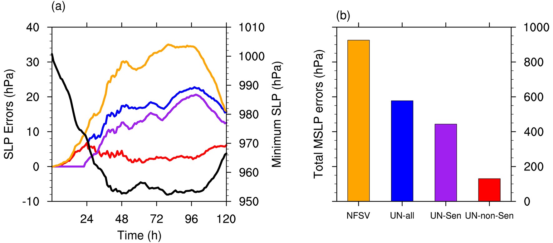Figure7. (a) The evolutionary curves of TC intensity of unperturbed run (black line) for the TC Soulik and its error evolutionary curve of TC intensity perturbed by the NFSV-type SST forcing error (orange); and the error evolutionary curves of TC intensity in the UN-all (blue), UN-Sen (purple), and UN-non-Sen (red) experiments; (b) the total error of the intensity [see Eq. (5)] for the TC simulation perturbed by the NFSV-type SST forcing error (orange), and the TC simulation in the UN-all (blue), UN-Sen (purple), and UN-non-Sen (red) experiments. Note that the maximum intensity error measured by MSLP forced by NFSV-type SST forcing errors can reach up to about 35 hPa during 72?96 h, which is comparable with the 23 hPa of the annual mean of root mean square errors (RMSEs) for TC center pressure forecasts with lead time 72 hrs.


Next, we will explore how the SST forcing errors in the H- and L-Sen periods influences TC intensity by perturbing the processes influencing TC intensity. To facilitate the calculation, we select only the 18 h, 114 h, and 42 h of the unperturbed run as representative of two L-Sen and one H-Sen periods to calculate the TC processes influencing TC intensity and associated simulation errors, where these three timings are all relative to the initial time of their respective time periods for 18 hrs.
We plot in Fig. 8 the azimuthal mean of surface latent heat flux errors, water vapor errors, and diabatic heating errors at 18 h and 114 h in the UN-non-Sen experiments, and at 42 h in the UN-Sen experiments. It is shown that the surface latent heat fluxes at all three timings yield negative errors, which are certainly caused by the negative SST forcing error of magnitude of ?1 K. Nevertheless, the surface latent heat flux error measured by its absolute value at 42 h in the UN-Sen experiment is larger than those at 18 h and 114 h; noting that especially large errors at 42 h occur closer to the inner core, which indicates that the significant decreases of surface latent heat flux in the UN-Sen experiments are due to the effects of the negative SST forcing errors and that the primary area of decrease occurs close to the inner core. According to the theory of wind induced surface heat exchange (WISHE; Emanuel et al., 1994), the surface latent heat flux is related to the wind speed associated with the TC intensity. Therefore, for the same magnitude of SST forcing errors, the stronger intensity of the TC in the unperturbed run will enhance the surface latent heat flux errors induced by the SST forcing errors, which explains why the surface latent heat flux errors in the UN-Sen experiments are larger than those in the UN-non-Sen experiments. The larger decrease of the surface latent heat flux in the UN-Sen experiments results in reduced water vapor in the boundary layer (especially closer to the inner core) of TC area by error, which will reduce the water vapor in the upper layers by the advective vertical term in the model, $\overline w q'$ ($\overline w $ indicates the vertical velocity of the unperturbed run and $q'$ denotes the negative water vapor error in lower layer, i.e. the reduced amount of water vapor in lower layer). Then the stronger secondary circulation of the TC in the unperturbed run during the H-Sen period will go on to favor a decrease of water vapor in the upper layers in the UN-Sen experiments, which reduces the diabatic heating compared to that in the UN-non-Sen experiments. As a result, the secondary circulation of the TC in the UN-Sen experiments is weaker at 42 h than that in the UN-non-Sen experiment due to the reduction of the diabatic heating [see Fig. 8 (d?f)], which, together with the weakened vertical velocity closer to the inner core, causes a large decreases of subsidence in the inner core, especially in the upper layer. The reduced subsidence by errors in the UN-Sen experiment indicates that the entry of high entropy air parcels into the warm core will be inhibited, which will cause considerable negative errors regarding the potential temperature in the upper layers in the UN-Sen experiment compared to that of the UN-non-Sen experiment. It is well known that there is a significant inverse correlation between TC warm core strength measured by the potential temperature in the upper layers and MSLP amplitude (indicating TC intensity); consequently a stronger warm core corresponds to stronger TC intensity (Chang and Wu, 2017). Thus, the TC intensity, as indicated by MSLP, is much lower in the UN-Sen experiment than in the UN-non-Sen experiments [see Fig. 8 (e)], indicating that the SST forcing error, with magnitude of ?1 K at each grid point in the UN-Sen experiment, tends to cause much larger simulation errors of the intensity of TC Soulik. This mechanism may explain why the SST forcing errors in the H-Sen period influence the TC intensity more significantly, and shed light on the physical reason behind the formation of the NFSV-type SST forcing errors.
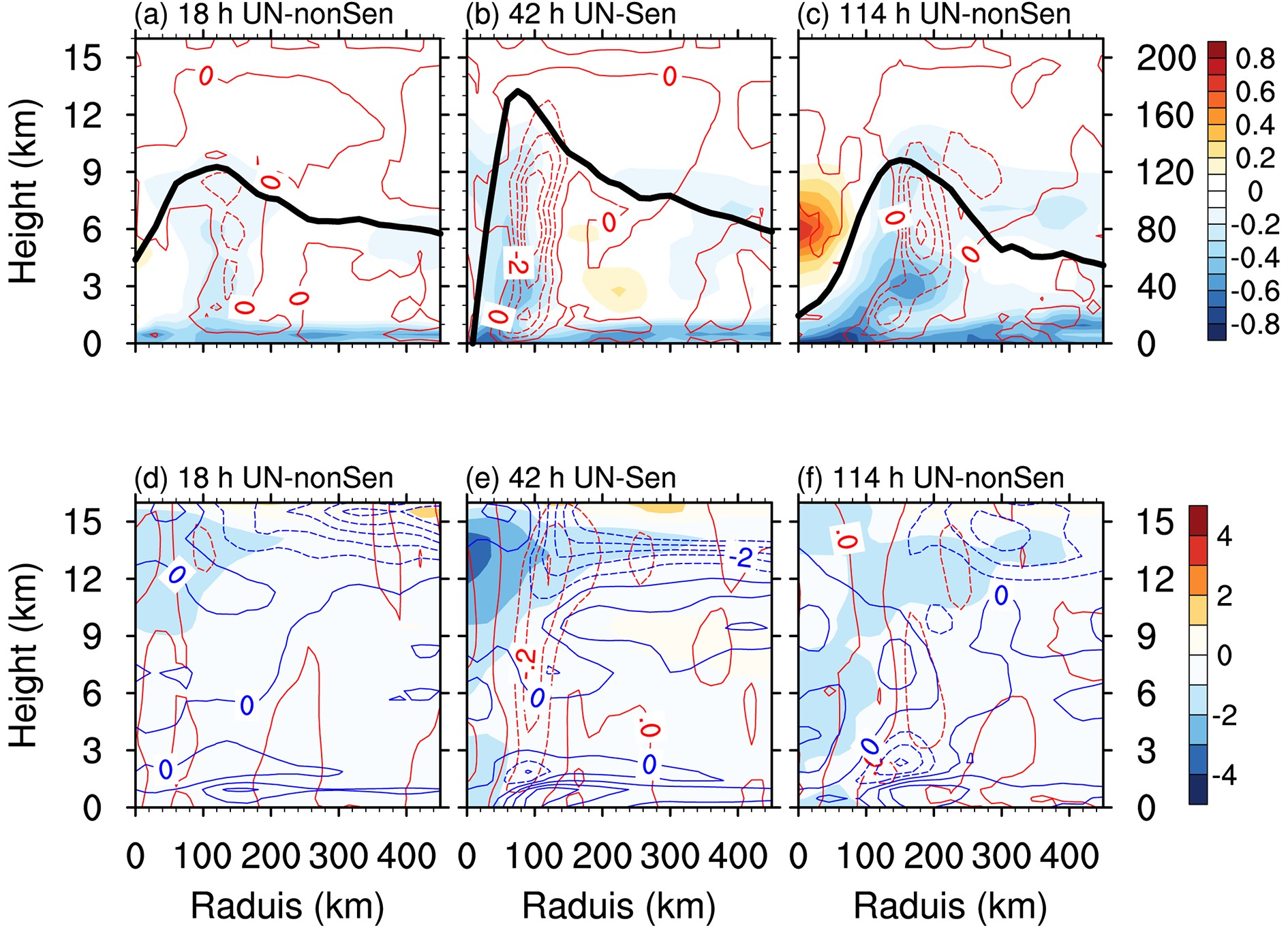Figure8. TC Soulik: azimuthal mean of surface latent heat flux errors (black lines, units: W m^?2), water vapor errors (shaded, units: g kg^?1), and diabatic heating errors (red contours, units: K h^?1, contour interval: 0.5 K h^?1) are plotted at (a) 18 h, (b) 42 h, and (c) 114 h; azimuthal mean of potential temperature errors (shaded, units: K), vertical velocity errors (red contours, units: m s^?1, contour interval: 0.1 m s^?1), and inflow errors (blue contours, units: m s^?1, contour interval: 1 m s^?1) are shown at (d) 18 h, (e) 42 h, (f) 114 h.



2 -->

4.3. The effect of inertial stability

The results in Table 3 and Fig. 5 show that the greatest sensitivities of TC intensity on SST forcing errors are associated with conditions of high inertial stability. We then pose the following two questions. How does the inertial stability affect TC intensities and through what mechanism does the high inertial stability in H-Sen period cause the SST forcing errors to yield such large intensity errors? Here, we show that the high inertial stability in the H-Sen period is favorable for the large growth of errors in TC intensity that is caused by the SST forcing errors. Furthermore, we suggest that this is caused by the response of the secondary circulation to the heat forcing. In the developments to follow, we address this issue by analyzing the Sawyer-Eliassen (SE) equation (Montgomery et al., 2006; Chen et al., 2018) through sensitivity experiments of the unperturbed run associated with TC Soulik with respect to the TC state in the UN-Sen experiment.
The application of the Boussinesq approximation, hydrostatic equilibrium and gradient wind balance, to the SE equation yields the transverse streamfunction which is written as follows (Montgomery et al., 2006; Chen et al., 2018).
here, r and z represent the radius and height, respectively; the overbar denotes the azimuthal mean; $\psi $ is streamfunction related to radial and vertical velocities with $u = - \left({1/r} \right)\left({\partial \psi /\partial z} \right)$ and $w = (1/r)(\partial \psi /\partial r)$, respectively; the coefficients A, B and C describe static stability, baroclinity, and inertial stability, which representing TC stability, and are given as follows.
where $\overline \theta $, $\overline v $ and $\overline \eta $ are azimuthal mean potential temperature, tangential velocity and absolute vertical vorticity, and g and ${\theta _{\rm{0}}}$ are the gravitational acceleration and the reference potential temperature (300 K), respectively; $\overline {{N^2}} $ is the azimuthally averaged Brunt-Vaisala frequency and $\overline \xi = {f_c} + 2\overline v /r$ is the local Coriolis parameter. The heating and momentum forcing terms on the rhs of Eq. (6) are defined as:
where the prime is the deviation from azimuthal mean; $\dot \theta $ is diabatic heating rate. The parameters A, B, C, $\overline Q $ and $\overline F $, are calculated according to the output of the WRF. Obviously, when we know the TC stability [i.e., A, B, and C in the Eqs. (7)?(9)] and the heating $\overline Q $ and momentum sources $\overline F $, the SE equation can be solved by standard successive over-relaxation (SOR; Press et al., 1992), where the momentum sources, $\overline F $, is the term associated with asymmetric advection, friction, subgrid-scale processes, and interpolation errors and so on.
The TC state at 42 h in the UN-Sen experiment (see the last sub-section) is used as input for the SE equation with the intent of diagnosing the role of inertial stability in response to the secondary circulation that is driven by diabatic heating. We replace the coefficient C, originally specific to the inertial stability of the unperturbed run, with that which is specific to the UN-Sen run. This adjustment yields resultant vertical and radial velocities that are shown in Fig, 9. It is shown that the vertical velocity in the convection area and the inflow and outflow measured by the radial velocity are all weaker, with the vertical velocity being especially weaker. In addition, it can be seen from Fig. 9 that the subsidence in the inner core becomes weaker. Collectively, these factors indicate that the secondary circulation becomes much weaker with the replacement of C (denoting the inertial stability) in the UN-Sen experiment while holding the TC states of static stability A, baroclinity B, heating forcing $\overline Q $, and momentum sources $\overline F $ unchanged. We further note that, replacing coefficient A (static stability) has little effect on the secondary circulation, and replacing coefficient B (baroclinity) only slightly affects the response of the secondary circulation in the boundary layer (corresponding figures are omitted here). We conclude that the inertial stability of the unperturbed run modulates the response of secondary circulation to the diabatic heating; and that the higher the inertial stability of the unperturbed run, the stronger the secondary circulation responds to the diabatic heating. To further clarify, high inertial stability will enhance the perturbation, regardless of whether it is positive or negative. In the last sub-section, we have shown that the secondary circulation in the UN-Sen experiments for TC Soulik becomes weaker due to the effect of negative SST forcing errors. From the results shown here, it is inferred that the high inertial stability of the unperturbed run in the H-Sen period enhances the weakening of secondary circulation in the UN-Sen experiments and a reduction of vertical velocity, which will cause considerable errors favoring for weaker subsidence which then leads to much greater negative errors regarding the potential temperature in the warm core. Ultimately, this results in a positive error of the MSLP which leads to an under-estimation of simulated TC intensity. Consequently, the high inertial stability of the unperturbed run during the H-Sen is favorable for the growth of the TC intensity errors caused by the SST forcing errors that occurred during this period, which is the suggested mechanism that contributes to the formation of the NFSV-type SST forcing errors.
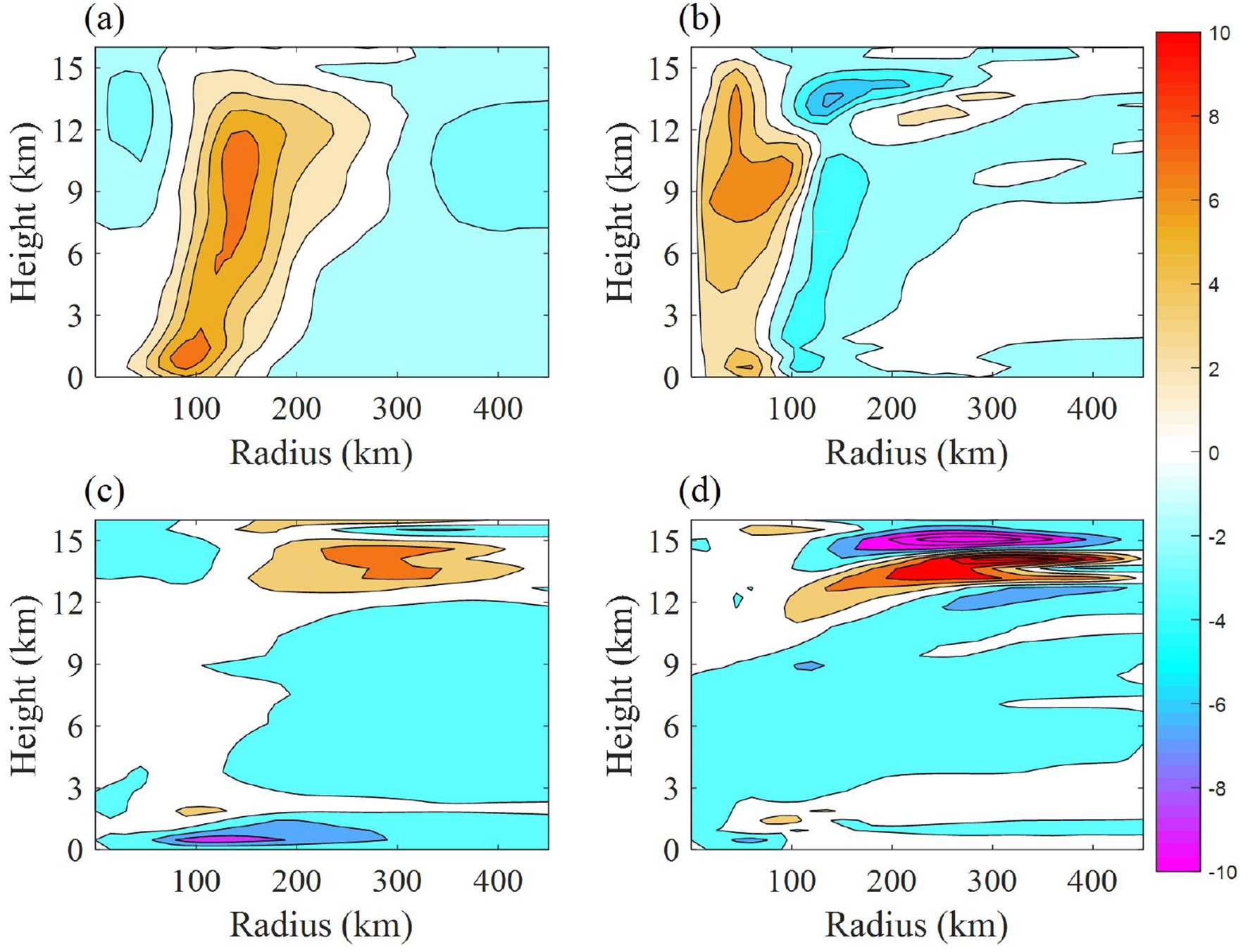Figure9. The azimuthal mean of (a) vertical velocity (units: 0.06 m s^?1) and (c) inflow (units: m s^?1) in the SE equation for the unperturbed run TC Soulik at time 42 h; the differences of the SE solution in (b) vertical velocity (units: 0.006 m s^?1) between the run in (a) and that with the coefficient C in the UN-Sen experiment and in (d) the inflow (0.1 m s^?1) between the run in (a) and that with the coefficient C in the UN-Sen experiment.

In section 4, we showed that the NFSV-type errors occur during the time period (i.e. the H-Sen period above) when the TCs present strong intensities,strong secondary circulations and high inertial stability. Moreover, the NFSV-type SST forcing errors tend to have the largest anomalies when the TCs are in the CTP, which identifies the time period when the intensity of TCs exhibit the strongest sensitivity to the SST forcing errors. In sections 4.2 and 4.3, we analyze TC Soulik as an example to explain why the aforementioned TC states are favorable for the growth of the intensity errors which are caused by the NFSV-type SST forcing error and we furthermore advance a physical mechanism which logically explains the the response of the secondary circulation to the NFSV-type SST forcing error. All evidence leads to the conclusion that the strongest sensitivity of TC intensity to the SST forcing errors along the TC track during the period when the TCs are of the CTP state. Therefore, if we manage to implement additional along-track SST observations during this particular time period, it would help to obtain a much more accurate SST forcing field for the WRF model, ultimately, reducing the simulation uncertainties of the TC intensity. If one uses a coupled model to simulate the TC, the along-track SST in this time period should be better simulated so as to greatly improve the TC intensity simulation skill.
In the present section, we continue to use the TC Soulik to explore how the NFSV-type SST forcing errors perturb the TC intensities by influencing the processes associated with TC intensification. From Fig. 7a, it is shown that, from about 24 h to 48 h, the intensity error caused by the NFSV-type SST forcing error produces larger growth rates (measured by the slope of the error evolutionary curve) than that in the UN-all experiment, which then causes larger intensity errors during the mature phase (i.e. from 48 h to 96 h) of TC Soulik despite the SST forcing errors in the UN-all experiment - having the same amplitude as in the NFSV-type SST forcing errors. We have known that the time period from 24 h to 48 h corresponds to the one when the NFSV-type SST forcing error possesses the largest anomalies and that the TC intensities are most sensitive to the SST forcing errors, which, as revealed in section 4, can explain why the NFSV-type SST forcing errors cause much larger intensity errors of a TC. We now pose the question, how does the NFSV-type SST forcing error influence the processes associated with the TC intensity and finally perturb the TC intensity?
Since we use the minimum MSLP to measure the intensity of TC, it is required to figure out the mechanism of the NFSV-type SST forcing error resulting in the change of the MSLP of the TC. As mentioned above, the MSLP of the TC is strongly correlated with the potential temperature in the upper layers of the TC. Therefore, we derive the potential temperature (PT) error tendency equation by examining the difference between the PT tendency equation component of the WRF model associated with unperturbed run and perturbed run mentioned above. The equation is given in Eq. (12):
Here, the overbar denotes the azimuthal mean, the star signifies the deviation from the azimuthal mean, the prime indicates the error caused by SST forcing error, and R is the residual term associated with unresolved processes as in section 4. However, for the residual term R, we cannot exactly separate the role of each of its inclusive processes. That is to say, the total effect of R is not of clear physics. For simplicity, we only considered the role of the terms with clear physics and do not analyze R here. The meanings of the other terms are listed in Table 4.

Term	Description
I	The tendency of the azimuthal mean of PT error;
II	The azimuthal mean diabatic heating error;
III	The radial advection of the azimuthal mean of PT by the azimuthal mean of radial velocity error;
IV	The radial advection of the azimuthal mean of PT error by the azimuthal mean of the perturbed radial velocity;
V	The azimuthal mean of the eddy component error of radial advection;
VI	The vertical advection of the azimuthal mean of PT error by the azimuthal mean of the perturbed vertical velocity;
VII	The vertical advection of the azimuthal mean of PT by the azimuthal mean of the vertical velocity error;
VIII	The azimuthal mean of the eddy component error of vertical advection.

Table4. The meaning of the terms in the PT error tendency equation


With the NFSV-type SST forcing error disturbed, we calculate the terms of Eq. (12) (confined in the eye region of TC within a round area centered at the simulated TC center with a radius of 50 km) for the TC Soulik. We find that the terms II, V and VII are much larger, which indicates that the diabatic heating error, eddy process error, and vertical advection of the PT by the vertical velocity error play an important role in generating PT error. These three terms are plotted in Fig. 10. It is found that the term VII (i.e. the vertical advection of the azimuthal mean of PT by the azimuthal mean of vertical velocity error) is negative especially in the upper layers (i.e. about 9 km above the surface for TC Soulik). Out of the three terms, Term VII is the largest when measured according to absolute value. This indicates that the term VII plays a dominate role in affecting PT, further noting that the vertical advection denoted by the term VII contributes to suppressing PT growth, especially when the TC is still intensifying just prior to the mature phase [i.e. from 30 to 48 h, which is within the window of the most sensitive period from 24 h to 48 h identified by the NFSV-type SST error]. Since the positive direction of the vertical PT gradient vector is upward, the negative contribution of the term VII to the PT growth mainly results from the positive error of vertical velocity (see Fig. 10f). As we know, in the eye region of TC, the vertical velocity is generally downward. Thus, the positive vertical velocity error reduces downward advection, and limits the amount of high entropy air parcels that enter the warm core which results in a decrease of TC intensity, ultimately yielding a negative error of TC intensity. Compared to term VII, term V, the error of eddy component of radial PT advection is much smaller, which indicates the SST forcing error has a negligible effect upon the asymmetric structure of the vortex associated with TC. Term 2, the diabatic heating error, is also relatively small, which may be due to the latent heat release occurring in the convection region instead of the eye region. In fact, as shown in section 4, the important effect of diabatic heating error, in the convection region, upon TC intensity simulation is uncertain. Therefore, the change of diabatic heating induced by the NSFV-type SST forcing error affects the warm core of TC in an indirect way.
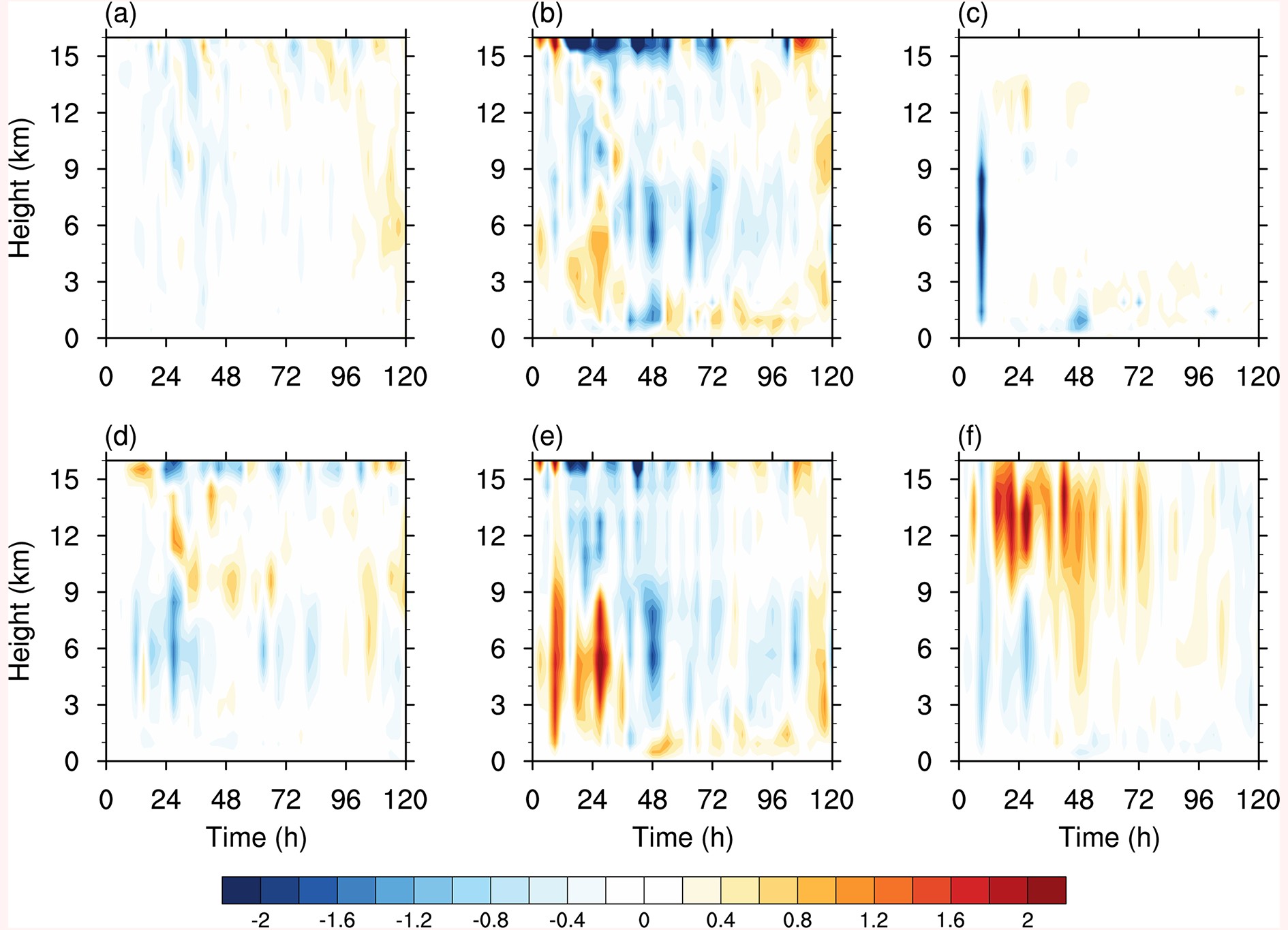Figure10. The time-height cross section of terms in potential temperature (PT) error tendency equation. PT error is caused by NFSV-type SST errors. All the terms are calculated by regional average within a round area centered at the simulated TC center with a radius of 50 km. (a) the term I; (b) the sum of rhs of Eq. (12) except the residual term; (c) the term II; (d) the term V; (e) the term VII; (f) the vertical velocity error (units: 0.1 m s^?1) caused by NFSV-type SST errors.


We plot in Fig. 11a the evolution of the absolute value of negative latent heat flux errors caused by the NFSV-type SST forcing error for TC Soulik. It is obvious that the latent heat flux error increases from 0 h to 48 h, especially within the interval of 24 h to 48 h due to the increase in surface wind consistent with the strong intensity of the TC during this period. Correspondingly, the water vapor error shows similar evolutionary behavior, with the largest reduction during the same sensitive period, from 24 h to 48 h. Then the water vapor advected into the inner core and upper layers is reduced as a consequence of the error, which causes large negative diabatic heating errors in the upper layers especially during the mature phase (i.e. from 48 h to 96 h) of TC Soulik, where the strong secondary circulation of the unperturbed run, as clarified in section 4, enhances the diabatic heating error in the upper layers induced by the water vapor error. Fig. 11b shows negative diabatic heating errors and vertical velocity errors forced by diabatic heating. It is shown that both the vertical velocity and the secondary circulation weaken, due to the effect of negative diabatic heating error. Despite the fact that the maximum of the negative diabatic heating errors do not occur during the most sensitive period of TC Soulik (see Fig. 11b), the strongest inertial stability of the unperturbed run during this period (see Fig. 6a) triggers a response of the secondary circulation to the diabatic heating and significantly increases the errors occurring in the secondary circulation, ultimately decreasing the vertical velocity, to the largest extent, during the most sensitive period from 24 h to 48 h. Particularly, we can see from Fig. 6a that the inertial stability is highest during the period from 24 h to 48 h and correspondingly, the vertical velocity error is the largest during this period. In response, the subsidence in the inner core is increased by a positive error (see Fig. 11c), especially from 24 h to 48 h. This results in reducing potential temperature of the upper layers of the inner core which leads to negative errors in potential temperature which accumulate rapidly from 24 h to 48 h (see Fig. 11c).The potential temperature then exhibits oscillatory behavior during the mature phase (i.e. from 48 h to 96 h) before dropping quickly from 96 h to 120 h, which coincides with the evolutionary behavior of the TC intensity error caused by the NFSV-type SST forcing error shown in Fig. 7a. Thus, the above mechanism interprets how the NFSV-type SST forcing errors perturb the intensity error.
Figure11. Evolution of (a) surface latent heating errors (black line; units: W m^?2) and water vapor errors (shaded; units: g kg^?1) regionally-averaged in a round centered at the simulated TC center within a radius of 300 km, (b) vertical velocity errors (red contours; units: m s^?1, contour interval: 0.1 m s^?1) and diabatic heating errors (shaded; units: 10 K h^?1) regionally-averaged in a ring area centered at the simulated TC center with the radii between 50 km and 150 km, and (c) subsidence errors (shaded; units: 0.1 m s^?1) and potential temperature errors (blue contours; units: K, contour interval: 2 K) regionally-averaged in a round centered at the simulated TC center within a radius of 50 km, which are all yielded by NFSV-type SST forcing errors.


Apart from the TC Soulik, we also explore the other ten TC cases with the strongest sensitivity occuring in the CTP of TCs. They have mechanisms similar to TC Soulik in the NFSV-type SST forcing errors affecting the TC intensity, except that some cases show signs opposite to those of the TC Soulik in the NFSV-type SST forcing errors and their resultant TC intensity uncertainties. Therefore, we can summarize the physical mechanisms as follows. When a NFSV-type SST forcing error with negative anomalies (or positive anomalies, depending on TC cases) occurs, it causes the surface latent heat flux and water vapor in low layers to decrease (increase). This further leads to a reduction (an increase) in diabatic heating which forces a weaker (stronger) secondary circulation and causes the downward vertical velocity in the eye region to decrease (increase). Eventually, the warm core of the TC becomes weaker (stronger) and the TC intensity tends to be under- (over-) estimated. In this process, the unperturbed run of the TC tends to present relatively strong intensity with the highest inertial stability and strong secondary circulation during the time period when the NFSV-type SST forcing error occurs. This property of the unperturbed run greatly enhances the latent heat flux errors in the low layers due to the effect of SST forcing error which goes on to increase the diabatic heating error, thereby, promoting a significant response from the secondary circulation before finally increasing the TC intensity error, most notably during the CTP.

The present study explores which TC features are affected the most by the SST forcing error that leads to TC intensity simulation uncertainties, with the intent of providing useful insights and ideas concerning target observation for SST forcing associated with TC intensity simulation. The approach of applyinga nonlinear forcing singular vector (NFSV) upon 12 TC cases for their 120-hour simulations are used to address this concern. The results show that the SST forcing errors of the NFSV structure often cause the largest simulation error of TC intensity. The NFSV-type SST forcing errors tend to be distributed along the TC track but are mainly concentrated during the time period when the TC is of strong intensity with strong secondary circulation and inertial stability, and exhibit positive or negative SST errors (which are dependent on the particular TC cases). Specifically, the NFSV-type SST forcing error of the TC tends to be dominated by the errors during the time period when the TC is in the CTP. Analysis of both the spatial and temporal distribution of those domains exhibiting model sensitivity (high correlation between SST forcing errors and TC intensity simulation errors) reveals that the critical time period of the TC response is consistent with the CTP of TC. This is identified by the NFSV-type SST forcing errors, which, by design, recognizes the time when the TC intensity is most sensitive to the SST forcing error. Therefore, if one manages to deploy additional SST observations during that particular time period of TC movement and assimilate them to the model SST forcing field, the TC intensity simulation level will be greatly improved. Even if a coupled model is used, the particular time period for targeting SST observations identified here will enable us to know when the SST should be preferentially well-simulated for improving the TC intensity simulation.
By sensitivity experiments and analysis of the SE equation, we show that the high inertial stability of the TC in the CTP determines the degree of the response of the secondary circulation to the SST forcing errors, which finally resolves to what extent the SST forcing errors influence the TC intensity. This indicates that if the SST forcing errors happen to occur during the CTP, the TC intensity will respond through the amplification or muting of the secondary circulation, thereby exerting a control upon subsidence in the core. The high inertial stability present during the CTP of the lifecycle of the TC greatly enhances this process and increases uncertainty of the TC intensity simulation at this time. Clearly, this argument explains the formation of the NFSV-type SST forcing errors for the TC intensity simulation.
By tracing the evolution of the TC intensity error, we suggest a mechanism that the NFSV-type SST forcing errors influence TC intensity. In particular, when the NFSV-type SST forcing error occurs along track and during the aforementioned CTP, the following events are likely to occur if the SST forcing error is negative (positive): it will cause both the low-layer atmospheric temperature and water vapor to be lower (higher) and consequently, the diabatic heating to decrease (increase). At this time, the secondary circulation, dominantly forced by the diabatic heating, becomes weaker (stronger) which causes the downward vertical velocity in the eye region of TC to become smaller (larger), finally causing the warm core of the TC to weaken (strengthen). Since the minimum MSLP is a proxy for TC intensity, coupled with the fact that this is strongly tied to the strength of the warm core, it follows that the TC intensity is under-(over-) estimated which presents large uncertainty. Additionally, the very large inertial stability of the TC the sensitive time period promotes a vigorous response of the secondary circulation to the SST forcing errors and causes a rapid accumulation of the TC intensity errors during this period, ultimately contributing the most to the total error of the TC intensity. This mechanism further illustrates that the NFSV-type SST forcing errors determine the time period and the region (where and when) targeted additional observations of SST forcing are needed to promote a more accurate TC intensity simulation.
Due to the destructive effects of TCs and associated danger, their direct observations, especially those of the ocean component, are often difficult to obtain and therefore very valuable. Even if some of the observations are retained, they are subject to large uncertainties. We have therefore researched,which physical variable, and within which region and time period, would be optimally suited for increasing the spatial density of observations with the intent of improving TC simulations and subsequently deepening the understanding of the TC system. We conclude that SST observations should be enhanced along the TC track, while the TC is strong, but still intensifying, just prior to the mature phase. This particular time period and region close to the eye of the TC provides a great logistical challenge to instrumentation personnel. The issue now becomes one of engineering and deployment. Can the observing equipment and instruments reach the sensitive area during stormy conditions and how will the instruments be deployed? The intent of this paper is restricted to isolating the spatio-temporal domain where the observations are needed and does not address the logistical issues related to instrument deployment, which is, at first glance, difficult and beyond the scope of the present study.
The present study used a version of the WRF model that has a horizontal resolution of 30 km×30 km. This coarse resolution, in of itself, can cause the simulation of TC intensity and structure to exhibit large biases. For example, the uncertainties of the RMW (radius of maximum wind) and the radius of the gale force wind cannot be adequately simulated after the SST forcing errors are superimposed. It then becomes apparent that the NFSV and its resultant sensitive area/ time period for target observations are based on biased TC simulations. Therefore, the evidence presented here discloses which time period and in which region the observations of the SST forcing are particularly important for improving the accuracy of the TC intensity simulation that contains biases. Despite this limitation, we put forward that the sensitive period for TC intensity simulation demonstrated here is still instructive, despite the model resolution that leaves much to be desired. Moreover, the primary results from our study are evidenced from 11 TC cases, all of which have the aforementioned sensitive time period/area in common. The reason why the TC Noul does not show coherent result is still unclear, which needs to be explored in future.
It is known that versions of the WRF model which use finer resolutions require more computational costs for the simulation of TC intensity. Furthermore, the computation of the NFSV is also expensive. When these two factors are combined, the TC simulations based upon a high-resolution WRF model with the NFSV computations, provide a challenge to computational resources. However, considering that the NFSV approach is useful for constructing theories for improving forecasting skill regarding TC intensity, we deem the computational investment worthy. We remain hopeful that the WRF model with finer resolution, together with a much more efficient algorithm for the NFSV approach will be used to accurately identify the sensitive period for target observation for not only SST forcing, but also for other relevant atmospheric variables, such as, initial wind field, initial temperature field, initial pressure field, and initial moisture field associated with TC intensity simulation. Such efforts can then fine tune the strategy for implementing target observations for TC intensity simulations. These considerations represent our subject areas for future investigations.
Acknowledgements. The authors appreciate the anonymous reviewers very much for their very useful comments and suggestions. This work was jointly sponsored by the National Nature Scientific Foundations of China (Grant Nos. 41930971) and the National Key Research and Development Program of China (Grant No. 2018YFC1506402) and the National Nature Scientific Foundations of China (Grant No. 41575061).