Ye PU¹,
Hongbo LIU^1,,,
Ruojing YAN^1,2,
Hao YANG^1,2,
Kun XIA¹,
Yiyuan LI¹,
Li DONG¹,
Lijuan LI¹,
He WANG¹,
Yan NIE^1,2,
Mirong SONG¹,
Jinbo XIE¹,
Shuwen ZHAO^1,2,
Kangjun CHEN¹,
Bin WANG¹,
Jianghao LI^1,2,
Ling ZUO^1,3

Corresponding author: Hongbo LIU,hongboliu@mail.iap.ac.cn;

1.State Key Laboratory of Numerical Modeling for Atmospheric Sciences and Geophysical Fluid Dynamics (LASG), Institute of Atmospheric Physics, Chinese Academy of Sciences, Beijing 100029, China
2.College of Earth and Planetary Sciences, University of Chinese Academy of Sciences, Beijing 100049, China
3.Department of Atmospheric Sciences, Yunnan University, Kunming 650504, China
Manuscript received: 2020-02-07
Manuscript revised: 2020-05-28
Manuscript accepted: 2020-06-18
Abstract:This paper describes the datasets from the Scenario Model Intercomparison Project (ScenarioMIP) simulation experiments run with the Chinese Academy of Sciences Flexible Global Ocean–Atmosphere–Land System Model, GridPoint version 3 (CAS FGOALS-g3). FGOALS-g3 is driven by eight shared socioeconomic pathways (SSPs) with different sets of future emission, concentration, and land-use scenarios. All Tier 1 and 2 experiments were carried out and were initialized using historical runs. A branch run method was used for the ensemble simulations. Model outputs were three-hourly, six-hourly, daily, and/or monthly mean values for the primary variables of the four component models. An evaluation and analysis of the simulations is also presented. The present results are expected to aid research into future climate change and socio-economic development.
Keywords: ScenarioMIP,
CMIP6,
CAS FGOALS-g3
摘要:本文介绍了中国科学院大气物理研究所研发的CAS FGOALS-g3模式在第六次国际耦合模式比较计划(CMIP6)的情景模式比较计划(ScenarioMIP)试验数据集。FGOALS-g3模式由8个共享社会经济路径(SSPs)驱动，它们分别具有不同的未来温室气体排放、浓度和土地利用情景。通过使用历史试验模拟结果进行初始化，模式完成了所有的第1层和第2层试验。模式输出数据包含四个分量模式的3小时、6小时、每日和/或每月平均的主要变量。文章对各组试验的模拟结果进行了初步的评估和分析。本文所涉及的试验结果将有助于对未来气候变化评估以及为社会经济发展制定相关政策提供数据支撑。
关键词:ScenarioMIP,
CMIP6,
CAS FGOALS-g3

HTML

--> --> -->

Climate change and sustainable development are at the frontier of international geoscience research in the 21st century. Their global impacts have made them two of the most important challenges facing human society today (Houghton et al., 1996, 2001; Ye et al., 2003). According to the Fifth Intergovernmental Panel on Climate Change (IPCC) Assessment Report, it is clear that human activity affects the climate system and recent anthropogenic emissions of greenhouse gases are the highest in history. Recent climatic changes have had a wide range of impacts on human and natural systems. Since 1950, many changes in extreme weather events and the climate have been observed, such as a decrease in extreme low temperatures, an increase in extreme high temperatures, extremely high sea levels, and heavy precipitation events in some regions (Alexander et al., 2006; Mudersbach et al., 2013; Wang and Fu, 2013). Continued emissions of greenhouse gases will lead to further warming and long-term changes in all components of the climate system, increasing the likelihood of serious, widespread, and irreversible impacts on human society and Earth’s ecosystems (AR5; IPCC, 2014).
Measurements of economic risk are science-based tools used by governments to make important decisions related to climate change. They are also core components of previous IPCC scientific assessment reports. To better measure the relationship between different socioeconomic development models and climate change risks, the IPCC developed scenario A (SA90) for the first assessment report (FAR) in 1990 (IPCC, 1990), IS92 for the third assessment report (TAR) in 1992 (IPCC, 1992), the SRE scenario for the TAR’s special report on emissions and the fourth assessment report (AR4; IPCC, 2000), and the Representative Concentration Pathway (RCP) for the fifth assessment report (van Vuuren et al., 2011). Phase 6 of the Coupled Model Intercomparison Project (CMIP6) uses six integrated assessment models (IAMs), various shared socioeconomic paths (SSPs), and the latest trends in anthropogenic emissions and land-use changes to generate new prediction scenarios. These scenarios form part of CMIP6 and are referred to as the Scenario Model Intercomparison Project (ScenarioMIP; O’Neill et al., 2016).
ScenarioMIP is a matrix combination of different SSPs and radiative forcing. An SSP describes possible future social development without the effects of climate change or climate policy (Zhang et al., 2019). O’Neill et al. (2016) gave a complete description of ScenarioMIP for CMIP6. For the analysis presented here, we briefly describe each SSP. A total of five pathways (i.e., SSP1, SSP2, SSP3, SSP4, and SSP5) are included in CMIP6, which consider the effects of population changes, economic growth, and urbanization (Calvin et al., 2017; Kriegler et al., 2017; Fricko et al., 2017; Fujimori et al., 2017; van Vuuren et al., 2017). Among the pathways, SSP1 is the most optimistic scenario and maintains sustainable development. In contrast, SSP5 assumes an energy intensive, fossil-fuel-based economy, although it also assumes relatively optimistic development. SSP2 is a middle pathway, which assumes current development trends continue in the future. SSP3 and SSP4 are the most undesirable pathways and assume unsustainable development trends, involving less investment in education and health, fast-growing populations, and increasing inequality. ScenarioMIP uses the IAMs to generate quantitative predictions of greenhouse gas emissions, atmospheric component concentrations, and land-use changes that may occur under different SSP energy scenarios. ScenarioMIP divides the experiments into two groups: Tier 1 and Tier 2. Tier 1 includes new SSP-based scenarios (SSP1-2.6, SSP2-4.5, SSP5-8.5) as continuations of the RCP2.6, RCP4.5, and RCP8.5 forcing levels, and an additional unmitigated forcing scenario (SSP3-7.0) with particularly high aerosol emissions and land-use change. Tier 2 includes additional scenarios of interest as well as additional ensemble members and long-term extensions (SSP1-1.9, SSP4-3.4, SSP4-6.0, SSP5-3.4-over) (O’Neill et al., 2016).
The Chinese Academy of Sciences Flexible Global Ocean–Atmosphere–Land System Model, GridPoint version 3 (CAS FGOALS-g3), developed by the State Key Laboratory of Numerical Modeling for Atmospheric Sciences and Geophysical Fluid Dynamics (LASG), Institute of Atmospheric Physics (IAP), Chinese Academy of Sciences (CAS), has completed the Tier 1 and 2 experiments of ScenarioMIP (Li et al., 2020a). Simulation results have been submitted to the Earth System Grid (ESG) data server (https://esgf-nodes.llnl.gov/projects/cmip6/). Section 2 provides detailed descriptions of the experimental design, model configuration, and output variables of the ScenarioMIP Tier 1 and 2 experiments performed using the CAS FGOALS-g3 model. Section 3 presents a preliminary model verification and future projections for each scenario. A brief usage note is provided in section 4.

2

-->

2.1. Model description

CAS FGOALS-g3 comprises the following five components:
(1) Atmospheric general circulation model (AGCM). The Gridpoint Atmospheric Model of IAP LASG, version 3 (GAMIL3) (Li et al. 2020b), is an updated version of GAMIL2 (Li et al., 2013).
(2) Oceanic general circulation model (OGCM). The LASG/IAP Climate Ocean Model (LICOM3) has been updated from LICOM2 (Liu et al., 2012; Lin et al., 2016). LICOM3 has performed the OMIP simulations and a detailed description of the results is given by Lin et al. (2020).
(3) Land model. The Land Surface Model of the Chinese Academy of Sciences (CAS-LSM), the land component of FGOALS-g3 with the same horizontal resolution as the atmospheric model, is based on the Community Land Model, version 4.5 (CLM4.5).
(4) Sea ice model. The sea ice model is the improved Los Alamos sea ice model, version 4.0, which uses the same grid as the oceanic model.
(5) Coupler. In FGOALS-g3, there are two optional couplers: CPL7, developed by the National Center for Atmospheric Research (NCAR) (Craig et al., 2012), and the Community Coupler, version 2 (C-Coupler2), developed by Tsinghua University (Liu et al., 2018).
A detailed description of CAS FGOALS-g3 is given in Li et al. (2020a).

2 -->

2.2. Experimental design

Following the requirements for ScenarioMIP experiments (O’Neill et al., 2016), we carried out simulations for eight scenarios (Experiment ID in Table 1). In these experiments, the external forcings, including greenhouse gas concentrations, ozone concentrations, anthropogenic aerosol optical properties and an associated Twomey effect, land-use changes, and solar irradiance, are all based on the SSP scenario. All experiments were initialized from 1 January 2015 (branch run from the end of the historical runs, which ended on 31 December 2014) and share the same physical scheme settings, which are exactly same as those of the historical run. Experiment variants are labelled; e.g., r1i1p1f1, indicating the realization, initialization, physical, and forcing indices. We used the branch run method for the Tier 1 and 2 SSP scenario simulations. For example, the label r1i1p1f1 indicates that the initial conditions are the outputs from the historical r1i1p1f1 branch run. Table 1 gives detailed descriptions of each experiment.

	Experiment ID	Variant Label	Description
Tier 1	SSP1-2.6 doi:10.22033/ESGF/CMIP6.3465	r1i1p1f1	Initialized from the historical r1i1p1f1 branch run. All external forcings were from the SSP1-2.6 scenario.
		r2i1p1f1	Initialized from the historical r2i1p1f1 branch run.
		r3i1p1f1	Initialized from the historical r3i1p1f1 branch run.
		r4i1p1f1	Initialized from the historical r4i1p1f1 branch run.
	SSP2-4.5 doi:10.22033/ESGF/CMIP6.3469	r1i1p1f1	Initialized from the historical r1i1p1f1 branch run. All external forcings were from the SSP2-4.5 scenario.
		r2i1p1f1	Initialized from the historical r2i1p1f1 branch run.
		r3i1p1f1	Initialized from the historical r3i1p1f1 branch run.
		r4i1p1f1	Initialized from the historical r4i1p1f1 branch run.
	SSP3-7.0 doi:10.22033/ESGF/CMIP6.3480	r1i1p1f1	Initialized from the historical r1i1p1f1 branch run. All external forcings were from the SSP3-7.0 scenario.
		r2i1p1f1	Initialized from the historical r2i1p1f1 branch run.
		r3i1p1f1	Initialized from the historical r3i1p1f1 branch run.
		r4i1p1f1	Initialized from the historical r4i1p1f1 branch run.
		r5i1p1f1	Initialized from the historical r5i1p1f1 branch run.
	SSP5-8.5 doi:10.22033/ESGF/CMIP6.3503	r1i1p1f1	Initialized from the historical r1i1p1f1 branch run. All external forcings were from the SSP5-8.5 scenario.
		r2i1p1f1	Initialized from the historical r2i1p1f1 branch run.
		r3i1p1f1	Initialized from the historical r3i1p1f1 branch run.
		r4i1p1f1	Initialized from the historical r4i1p1f1 branch run.
Tier 2	SSP1-1.9 doi:10.22033/ESGF/CMIP6.3462	r1i1p1f1	Initialized from the historical r1i1p1f1 branch run. All external forcings were from the SSP1-1.9 scenario.
	SSP4-3.4 doi:10.22033/ESGF/CMIP6.3493	r1i1p1f1	Initialized from the historical r1i1p1f1 branch run. All external forcings were from the SSP4-3.4 scenario.
	SSP5-3.4-over doi:10.22033/ESGF/CMIP6.3499	r1i1p1f1	Initialized from the historical r1i1p1f1 branch run. All external forcings were from the SSP5-3.4-over scenario.
	SSP4-6.0 doi:10.22033/ESGF/CMIP6.3496	r1i1p1f1	Initialized from the historical r1i1p1f1 branch run. All external forcings were from the SSP4-6.0 scenario.

Table1. ScenarioMIP experiment descriptions.


We used the model outputs for the period 2015–2100 in our analysis. Following the requirements of CMIP6 (Martin et al., 2020), monthly mean values for the primary variables of each component model were output. To investigate predicted extreme weather events in each scenario, the atmospheric component also provides additional 6-h and 3-h high-frequency outputs for some variables, including precipitation, specific humidity, and near-surface air temperature, for both future predictions and the historical runs. Details of the primary outputs and diagnostic variables for each component model are given in Tables 2–5.

Variable Name	Description	Output Frequency
cl	Percentage Cloud Cover	Monthly
cli	Mass Fraction of Cloud Ice	Monthly
clivi	Ice Water Path	Monthly
clt	Total Cloud Cover Percentage	3-h*, Daily, Monthly
clw	Mass Fraction of Cloud Liquid Water	Monthly
clwvi	Condensed Water Path	Monthly
evspsbl	Evaporation Including Sublimation and Transpiration	Monthly
hfls	Surface Upward Latent Heat Flux	3-h*, Daily, Monthly
hfss	Surface Upward Sensible Heat Flux	3-h*, Daily, Monthly
hur	Relative Humidity	Daily, Monthly
hurs	Near-Surface Relative Humidity	6-h*, Daily, Monthly
hursmax	Daily Maximum Near-Surface Relative Humidity	Daily
hursmin	Daily Minimum Near-Surface Relative Humidity	Daily
hus	Specific Humidity	6-h*, Daily, Monthly
huss	Near-Surface Specific Humidity	3-h*, Daily, Monthly
mc	Convective Mass Flux	Monthly
o3	Mole Fraction of O3	Monthly
pfull	Pressure at Model Full-Levels	6-h*, Monthly
phalf	Pressure on Model Half-Levels	Monthly
pr	Precipitation	3-h*, 6-h*, Daily, Monthly
prc	Convective Precipitation	3-h*, Daily, Monthly
prhmax	Maximum Hourly Precipitation Rate	6-h*
prsn	Snowfall Flux	3-h*, Daily, Monthly
prw	Water Vapor Path	Monthly
ps	Surface Air Pressure	3-h*, 6-h*, Monthly
psl	Sea Level Pressure	6-h*, Daily, Monthly
rlds	Surface Downwelling Longwave Radiation	3-h*, Daily, Monthly
rldscs	Surface Downwelling Clear-Sky Longwave Radiation	3-h*, Monthly
rls	Net Longwave Surface Radiation	Daily
rlus	Surface Upwelling Longwave Radiation	3-h*, Daily, Monthly
rlut	TOA Outgoing Longwave Radiation	Daily, Monthly
rlutcs	TOA Outgoing Clear-Sky Longwave Radiation	Monthly
rsds	Surface Downwelling Shortwave Radiation	3-h*, Daily, Monthly
rsdscs	Surface Downwelling Clear-Sky Shortwave Radiation	3-h*, Monthly
rsdsdiff	Surface Diffuse Downwelling Shortwave Radiation	3-h*
rsdt	TOA Incident Shortwave Radiation	Monthly
rss	Net Shortwave Surface Radiation	Daily
rsus	Surface Upwelling Shortwave Radiation	3-h*, Daily, Monthly
rsuscs	Surface Upwelling Clear-Sky Shortwave Radiation	3-h*, Monthly
rsut	TOA Outgoing Shortwave Radiation	Monthly
rsutcs	TOA Outgoing Clear-Sky Shortwave Radiation	Monthly
rtmt	Net Downward Radiative Flux at Top of Model	Monthly
sfcWind	Near-Surface Wind Speed	6-h*, Daily, Monthly
sfcWindmax	Daily Maximum Near-Surface Wind Speed	Daily
ta	Air Temperature	6-h*, Daily, Monthly
tas	Near-Surface Air Temperature	3-h*, 6-h*, Daily, Monthly
tasmax	Daily Maximum Near-Surface Air Temperature	Daily, Monthly
tasmin	Daily Minimum Near-Surface Air Temperature	Daily, Monthly
tauu	Surface Downward Eastward Wind Stress	Monthly
tauv	Surface Downward Northward Wind Stress	Monthly
ts	Surface Temperature	Monthly
ua	Eastward Wind	6-h*, Daily, Monthly
va	Northward Wind	6-h*, Daily, Monthly
wap	Omega (= dp/ dt)	6-h*, Daily, Monthly
zg	Geopotential Height	Daily, Monthly

Table2. AGCM output variables from FGOALS-g3 for the ScenarioMIP experiments. TOA means top of atmosphere; * represents additional high-frequency output variables.

Variable Name	Description	Output Frequency
friver	Water Flux into Sea Water from Rivers	Monthly
hfbasin	Northward Ocean Heat Transport	Monthly
hfds	Downward Heat Flux at Sea Water Surface	Monthly
hflso	Surface Downward Latent Heat Flux	Monthly
hfsso	Surface Downward Sensible Heat Flux	Monthly
mlotst	Ocean Mixed Layer Thickness Defined by Sigma T	Monthly
msftbarot	Ocean Barotropic Mass Stream Function	Monthly
msftmz	Ocean Meridional Overturning Mass Stream Function	Monthly
msftmzmpa	Ocean Meridional Overturning Mass Stream Function Due to Parameterized Mesoscale Advection	Monthly
rlntds	Surface Net Downward Longwave Radiation	Monthly
rsntds	Net Downward Shortwave Radiation at Sea Water Surface	Monthly
so	Sea Water Salinity	Monthly
soga	Global Mean Sea Water Salinity	Monthly
sos	Sea Surface Salinity	Monthly
thetao	Sea Water Potential Temperature	Monthly
thetaoga	Global Average Sea Water Potential Temperature	Monthly
tos	Sea Surface Temperature	Monthly
tossq	Square of Sea Surface Temperature	Monthly
umo	Ocean Mass X Transport	Monthly
uo	Sea Water X Velocity	Monthly
vmo	Ocean Mass Y Transport	Monthly
vo	Sea Water Y Velocity	Monthly
vsf	Virtual Salt Flux into Sea Water	Monthly
wfo	Water Flux into Sea Water	Monthly
wmo	Upward Ocean Mass Transport	Monthly
wo	Sea Water Vertical Velocity	Monthly
zos	Sea Surface Height Above Geoid	Monthly
zossq	Square of Sea Surface Height Above Geoid	Monthly

Table3. OGCM output variables from FGOALS-g3 for the ScenarioMIP experiments.

Variable Name	Description	Output Frequency
evspsblsoi	Water Evaporation from Soil	Monthly
evspsblveg	Evaporation from Canopy	Monthly
gwt	Groundwater Intake	Monthly
mrfso	Soil Frozen Water Content	Monthly
mrro	Total Runoff	Monthly
mrros	Surface Runoff	Monthly
mrso	Total Soil Moisture Content	Monthly
mrsos	Moisture in Upper Portion of Soil Column	Monthly
prveg	Precipitation onto Canopy	Monthly
tsl	Temperature of Soil	Monthly
frostdp	Frost Deep	Monthly
snc	Snow Area Percentage	Monthly
snd	Snow Depth	Monthly
thawdp	Thaw Depth	Monthly

Table4. Land model output variables from FGOALS-g3 for the ScenarioMIP experiments.

Variable Name	Description	Output Frequency
sfdsi	Downward Sea Ice Basal Salt Flux	Monthly
siconc	Sea-Ice Area Percentage (Ocean Grid)	Monthly
sidconcdyn	Sea-Ice Area Percentage Tendency Due to Dynamics	Monthly
sidconcth	Sea-Ice Area Percentage Tendency Due to Thermodynamics	Monthly
sidivvel	Divergence of the Sea-Ice Velocity Field	Monthly
sidmassdyn	Sea-Ice Mass Change from Dynamics	Monthly
sidmassgrowthbot	Sea-Ice Mass Change Through Basal Growth	Monthly
sidmassgrowthwat	Sea-Ice Mass Change Through Growth in Supercooled Open Water (Frazil)	Monthly
sidmasslat	Lateral Sea-Ice Melt Rate	Monthly
sidmassmeltbot	Sea-Ice Mass Change Through Bottom Melting	Monthly
sidmassmelttop	Sea-Ice Mass Change Through Surface Melting	Monthly
sidmasssi	Sea-Ice Mass Change Through Snow-to-Ice Conversion	Monthly
sidmassth	Sea-Ice Mass Change from Thermodynamics	Monthly
siflcondtop	Net Conductive Heat Flux in Ice at the Surface	Monthly
sifllatstop	Net Latent Heat Flux over Sea Ice	Monthly
sifllwdtop	Downwelling Longwave Flux over Sea Ice	Monthly
sifllwutop	Upwelling Longwave Flux over Sea Ice	Monthly
siflsenstop	Net Upward Sensible Heat Flux over Sea Ice	Monthly
siflsensupbot	Net Upward Sensible Heat Flux Under Sea Ice	Monthly
siflswdbot	Downwelling Shortwave Flux Under Sea Ice	Monthly
siflswdtop	Downwelling Shortwave Flux over Sea Ice	Monthly
siflswutop	Upwelling Shortwave Flux over Sea Ice	Monthly
siforcecoriolx	Coriolis Force Term in Force Balance (X-Component)	Monthly
siforcecorioly	Coriolis Force Term in Force Balance (Y-Component)	Monthly
siforceintstrx	Internal Stress Term in Force Balance (X-Component)	Monthly
siforceintstry	Internal Stress Term in Force Balance (Y-Component)	Monthly
sipr	Rainfall Rate over Sea Ice	Monthly
sishevel	Maximum Shear of Sea-Ice Velocity Field	Monthly
sisnconc	Snow Area Percentage	Monthly
sistrxdtop	X-Component of Atmospheric Stress on Sea Ice	Monthly
sistrxubot	X-Component of Ocean Stress on Sea Ice	Monthly
sistrydtop	Y-Component of Atmospheric Stress on Sea Ice	Monthly
sistryubot	Y-Component of Ocean Stress on Sea Ice	Monthly
sitemptop	Surface Temperature of Sea Ice	Monthly
sitimefrac	Fraction of Time Steps with Sea Ice	Monthly
siu	X-Component of Sea-Ice Velocity	Monthly
siv	Y-Component of Sea-Ice Velocity	Monthly
sndmassmelt	Snow Mass Rate of Change Through Melt	Monthly
sndmasssi	Snow Mass Rate of Change Through Snow-to-Ice Conversion	Monthly
sndmasssnf	Snow Mass Change Through Snowfall	Monthly

Table5. Sea ice model output variables from FGOALS-g3 for the ScenarioMIP experiments.


We used the following observational datasets for the model validation: Global Precipitation Climatology Project (GPCP, version 2.3) monthly data (Adler et al., 2003), HadCRUT4 monthly mean near-surface temperatures (Morice et al., 2012), China Merged Surface Temperature data (Yun et al., 2019), and the Arctic and Antarctic sea ice area records provided by the National Snow and Ice Data Center (NSIDC; http://nsidc.org/arcticseaicenews/sea-ice-tools/). The ensemble means from the historical runs (six members) and Tier 1 SSP experiments (see Table 1 for ensemble sizes) were used in our analysis. The base period for each anomaly analysis was 1980–2009.

Reasonable reproductions of the past climate form the basis of the future projections generated by most climate models. In our historical runs, the trend of increasing surface temperature (i.e., global warming; 1980–2009 base period is adopted) since 1980 is well reproduced, and the fluctuation around 1990–1995 (related to volcano activities) is also well captured (Fig. 1a). This warming trend remains for all ScenarioMIP experiments until the 2030s when the projections diverge. The surface temperature increase remains roughly linear for high-emission scenarios with large radiative forcings, especially for SSP5-8.5, but also for SSP3-7.0, SSP4-6.0, and SSP2-4.5. By 2100, the positive anomaly is projected to reach 3.2°C (SSP5-8.5), 2.8°C (SSP3-7.0), 1.8°C (SSP4-6.0), or 1.4°C (SSP2-4.5). In contrast, there is no significant temperature increase projected for SSP5-3.4-over, SSP4-3.4, or SSP1-2.6, and a decreasing trend is even projected for SSP1-1.9. The positive anomaly in 2018 is 0.6°C but decreases to 0.4°C after 2050 for SSP1-1.9.
Figure1. Global mean (a) surface air temperature anomaly (units: °C) and (b) precipitation anomaly (units: mm d^?1) time series from observations (black and deep red lines), historical runs (red line) for 1980–2014, and eight SSP scenario experiments for 2015–2100. The base period is 1980–2009.


During the period 1980–2016, the observed global precipitation (GPCP) follows an increasing trend but with large annual fluctuations (Fig. 1b). The FGOALS-g3 model captures this increasing trend, but with less pronounced annual fluctuations. This is reasonable because the result of FGOALS-g3 is the ensemble mean, which smooths some model internal variability. Under all scenarios, the precipitation increases until 2050 when precipitation variability increases and results diverge among the scenarios, as was the case for the surface temperature trends (Fig. 1a). For SSP1-1.9, the precipitation decreases after 2050, and eventually returns to the values of the 2000s and 2010s. For SSP4-3.4 and SSP5-3.4-over, the increasing tends are not significant. By 2100, the anomaly reaches 0.06 mm d^?1 for scenarios SSP2-4.5 and SSP4-6.0, and exceeds 0.10 mm d^?1 for scenarios SSP3-7.0 and SSP5-8.5.
Consistent with the results shown in Fig. 1a, the annual mean global surface temperature follows an overall increasing trend over the period 2070–99 relative to the base period, as radiative forcing increases. However, large spatial discrepancies for the same emission and land-use scenarios exist in the simulations from each experiment (Fig. 2). In general, the surface temperature over the Arctic and high-latitude regions of the NH presents the strongest warming signals, with amplitudes of 1.0°C to >5.0°C for the SSP1-1.9 to SSP5-8.5 scenarios. The surface warming over the continents is generally higher than over the oceans, particularly for the Tibetan and Brazilian plateaus. Although ocean surface warming remains relatively weak, the equatorial East–Central Pacific shows an El Ni?o-like warm tongue for SSP4-3.4 and the last four scenario simulations (Figs. 2c and e–h). The differences in regional patterns of warming are consistent with expectations and previous results. Note that although a global warming trend exists under each scenario, the North Atlantic Ocean is an exception. The northwest–southeast belt-shaped “warm hole” (i.e., cooling anomaly) in this region even strengthens with increased radiative forcing and reaches ?5.0°C for SSP4-6.0 (Fig. 2f). This phenomenon has been observed in other simulation studies (Gervais et al., 2019), and may be related to Arctic sea ice melting and resulting changes to ocean circulation patterns, such as the Atlantic Meridional Overturning Circulation (AMOC). We will describe them in the following contents.
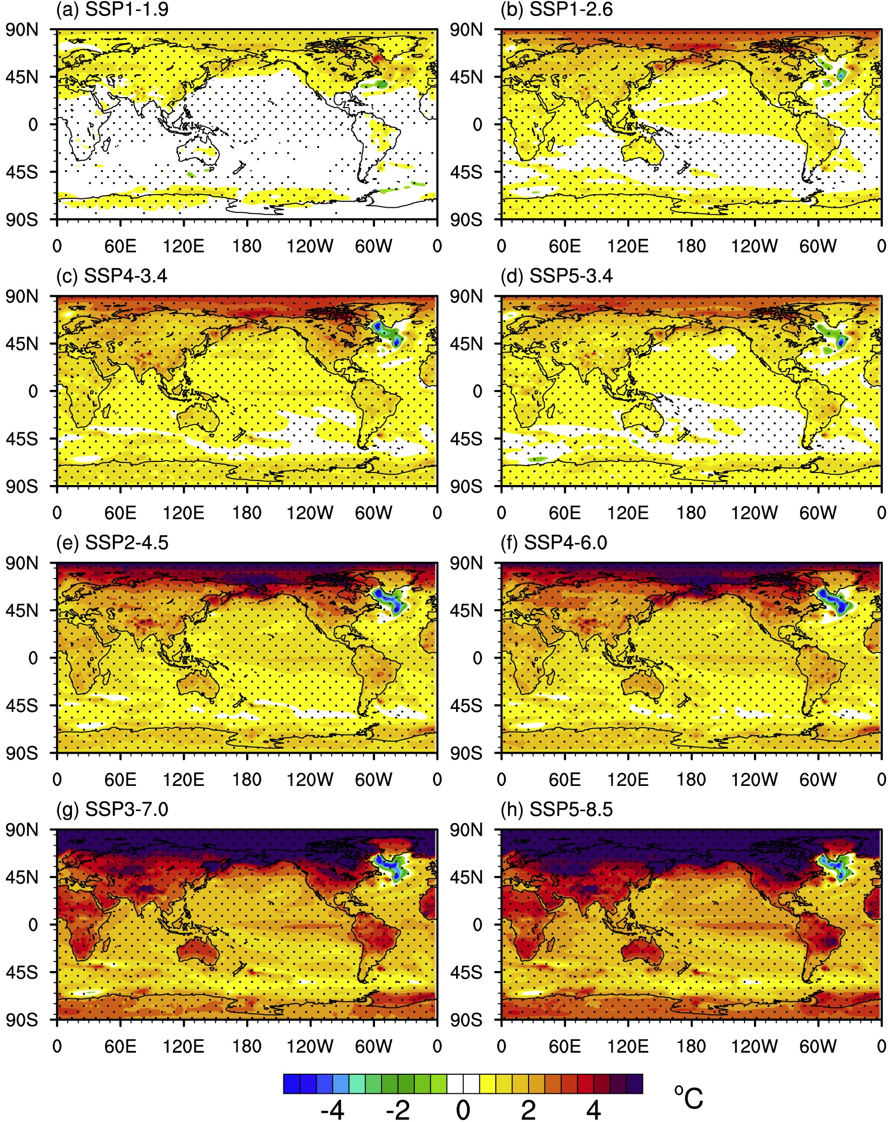Figure2. Annual mean global surface temperature difference (units: °C; 2070–2099 minus 1980–2009) between the eight ScenarioMIP experiments (2070–2099) and historical runs (1980–2009) for scenarios (a) SSP1-1.9, (b) SSP1-2.6, (c) SSP4-3.4, (d) SSP5-3.4-over, (e) SSP2-4.5, (f) SSP4-6.0, (g) SSP3-7.0, and (h) SSP5-8.5. Black dots denote the results significant at the 95% confidence level (similarly for Figs. 3 and 4).


The projected annual mean precipitation shows large variations in the tropical and subtropical regions of both the NH and SH (Fig. 3). Between 2070 and 2099, there is a narrow quasi-east–west belt of increased rainfall over the equatorial Pacific with large amounts of precipitation to the east of the Maritime Continent. The positive rainfall anomalies increase from 0.5 mm d^?1 to >3.0 mm d^?1 as the scenario varies from lower to higher future forcing. In contrast, the tropical Indian Ocean, subtropical southwestern Pacific, tropical western Atlantic, and northern South America all show decreases in rainfall of ?0.5 to ?1.5 mm d^?1. Rainfall anomalies present an obvious dipole feature in the tropical Indian ocean in all scenarios. Lower rainfall intensities in these regions are associated with greater radiative forcing.
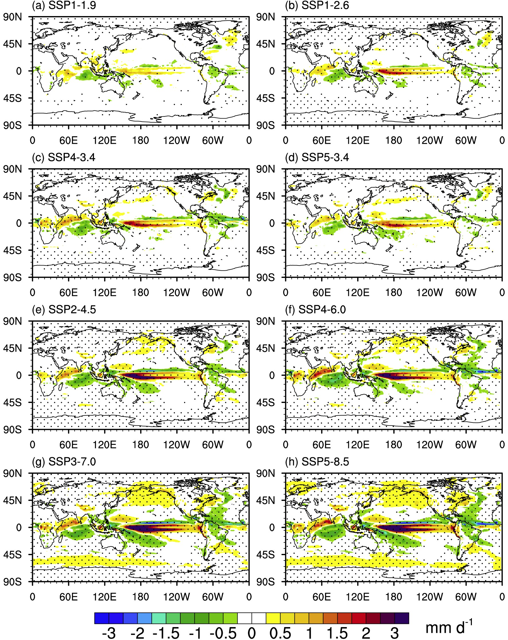Figure3. As in Fig. 2, but for annual mean global precipitation (units: mm d^?1).


The spatial distributions of winter snow cover over the NH for the period 2070–2099 relative to the base period for eight scenarios are shown in Fig. 4. Clear negative anomalies are evident in the NH under the various emission scenarios. Western Europe and southern North America experience the most significant decrease. With increasing carbon dioxide concentrations and anthropogenic radiative forcing, these negative anomalies grow. For SSP3-7.0 and SSP5-8.5, most areas north of 30°N show negative anomalies, with values less than ?0.2 over Eurasia and North America (Figs. 4g and h). Results suggest that to maintain snow cover over the NH, it will be important to control greenhouse gas emissions in the future.
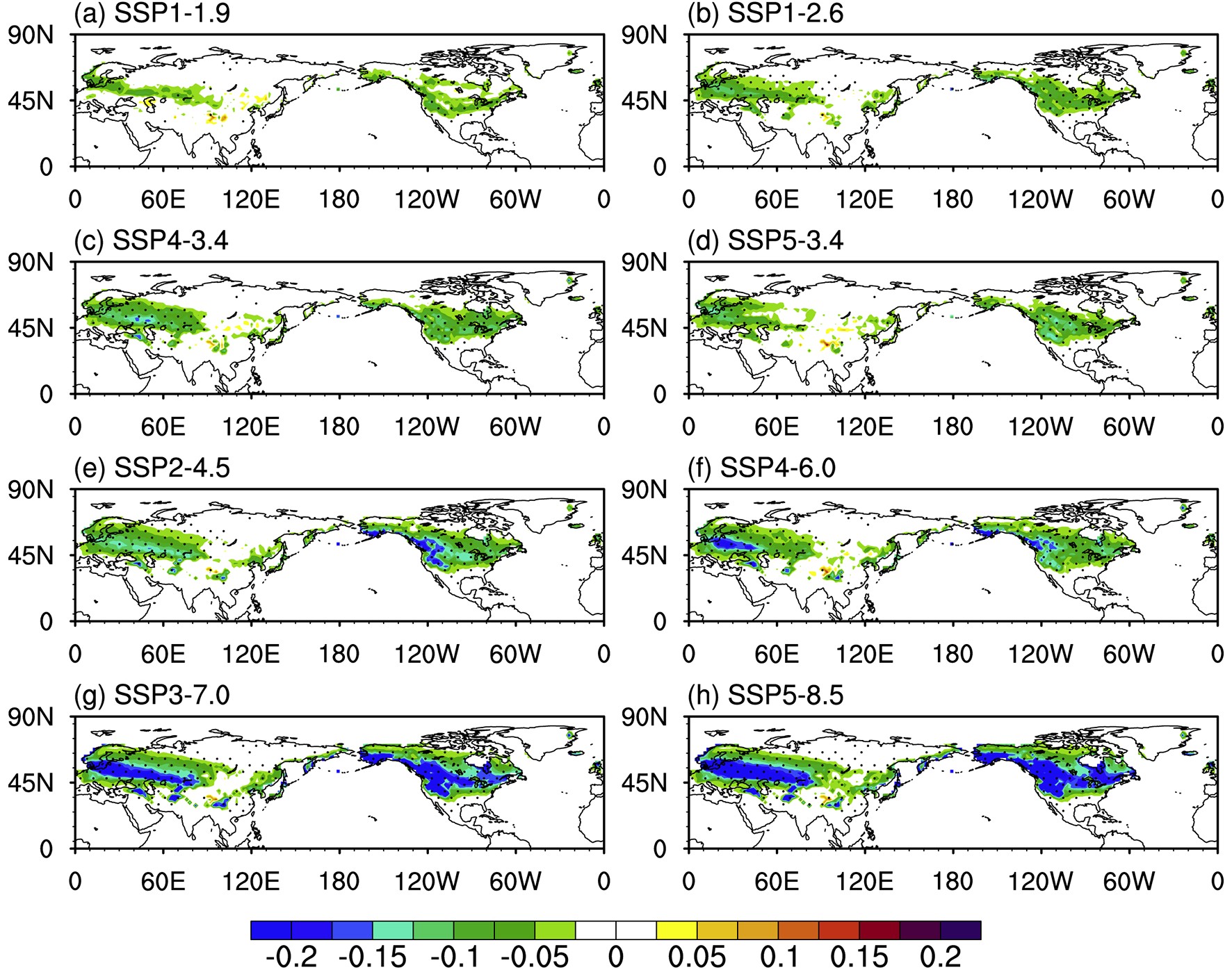Figure4. As in Fig. 2, but for the spatial distribution of winter snow cover fraction over the NH.


The AMOC plays an important role in regulating the climate by transporting heat northward in the Atlantic and thus maintaining the warmth of the NH. The annual mean maximum volume transport stream function at 26.5°N [units: Sverdrups (Sv)] in the Atlantic is used to measure the intensity of the AMOC. The historical and eight scenario simulations of the AMOC are shown in Fig. 5. From 1980 to 2015, the simulated AMOC from historical runs maintains an intensity of approximately 27.0 Sv, with a weak increase during the 1980s and a decrease in the early 1990s. Similar to surface temperature, the projected AMOC shows an overall weakening trend from 2015 to 2100 for SSP2-4.5, SSP4-6.0, SSP3-7.0, and SSP5-8.5. By 2100, the AMOC shows a decrease in intensity of 26% (37%) for SSP2-4.5 and SSP4-6.0 (SSP3-7.0 and SSP5-8.5). Due to the internal variability of AMOC, the regulation of deep water formation in the Greenland–Iceland–Norwegian Seas and Arctic sea ice melting, the projected AMOC shows large fluctuations under small-to-medium radiative forcing scenarios. This is similar to the results of FGOALS-g2 (Huang et al., 2014). For example, in the 2090s, the AMOC exhibits a strong rebound with a 4% intensity increase relative to 2014 values for SSP1-1.9. For SSP1-2.6, SSP4-3.4, and SSP5-3.4-over, the AMOC also rebounds, but to a lesser extent than for SSP1-1.9.
Figure5. AMOC (units: Sv) time series from historical runs (red line) for 1980–2014 and eight SSP scenario experiments for 2015–2100.


Figure 6 presents the sea ice area (SIA) anomaly time series over both hemispheres for the NSIDC observations, the historical runs, and the eight ScenarioMIP experiments. Overall, the variation of the SIA over the SH is greater than in the NH in both observations and simulations. The observed SIA over the NH first rises at the end of the 1980s and then gradually decreases over the subsequent 30 years (Fig. 6a). In contrast, the SIA over the SH has continuously increased, with relatively large annual variations, since 1980, and reached a peak around 2014 before decreasing sharply to its lowest point in 2017. The SIA anomalies associated with the historical runs over the NH are more consistent with the observations (i.e., they follow a decreasing trend), but show large discrepancies over the SH, especially between 2008 and 2014 (Fig. 6b). The rate of projected SIA decay over the NH is the largest for SSP5-8.5, followed by SSP3-7.0. The projected SIA over the NH is constant for SSP1-1.9, SSP1-2.6, SSP4-3.4, and SSP5-3.4-over, and even increases in the mid-21st century for SSP1-1.9. Although the SIA over the SH exhibits similar variations to those over the NH for each SSP, the decay rate decreases (e.g., for SSP5-8.5 and SSP3-7.0) and the amplitude of the annual fluctuations increases for all ScenarioMIP experiments.
Figure6. SIA anomaly (units: 10⁶ km²) time series for the (a) NH and (b) SH from NSIDC observations (1980–2019), historical runs (1980–2014), and eight ScenarioMIP runs (2015–2100). The base period is 1980–2009.

The AGCM and land surface model use the same horizontal resolution; i.e., an equal area-weighted 180 × 80 horizontal grid in the zonal and meridional directions. The OGCM and sea ice model use the same tripolar 360 × 218 grid. The model outputs on their native grids have been saved and transformed to the Climate Model Output Rewriter (CMOR) file structure as required by CMIP6. According to the standard of CMOR, each variable is stored in a separate file. The dataset format is Network Common Data Form (NetCDF), version 4. The data can be downloaded from CMIP6 website.
Acknowledgements. This study was supported by the National Key Research and Development Program of China (Grant Nos. 2017YFA0603903, 2017YFA0603901, and 2017YFA0603902), the Strategic Priority Research Program of Chinese Academy of Sciences (Grant No. XDB42010404) and the National Basic Research (973) Program of China (Grant Nos. 2015CB954102).

The data that support the findings of this study are available at https://esgf-node.llnl.gov/projects/cmip6/. The citation for ScenarioMIP is “CAS FGOALS-g3 model output prepared for CMIP6 ScenarioMIP. Earth System Grid Federation. Doi :10.22033/ESGF/CMIP6.2056”. Users are encouraged to download and share the data mentioned in this paper. All the datasets are free.

No potential conflicts of interest are reported by the authors.
Open Access This article is distributed under the terms of the Creative Commons Attribution 4.0 International License (http://creativecommons.org/licenses/by/4.0/), which permits unrestricted use, distribution, and reproduction in any medium, provided you give appropriate credit to the original author(s) and the source, provide a link to the Creative Commons license, and indicate if changes were made.