HTML
--> --> -->In this study, we show that stratospheric ozone recovery leads to decreases in cloud at SH high latitudes, and that the radiative effects of these cloud decreases also play important roles in causing ocean surface cooling and increasing Antarctic sea-ice.
The model used here is the Community Atmosphere Model, version 4 (CAM4) (Neale et al., 2013). To distinguish ozone-induced cloud radiative effects on sea-ice from the dynamic effects that have been studied in previous works (Sigmond and Fyfe, 2010; Bitz and Polvani, 2012; Smith et al., 2012), CAM4 is coupled with a slab ocean of 50 m in depth and a thermodynamic sea-ice model. Therefore, neither sea-ice formation nor melting involves sea-ice dynamics or ocean heat transports. Both simulations are run for 50 years to reach equilibrium, and the averages of the simulation results over the last 30 years are used for analysis. The simulations here are similar to those in Smith et al. (2012), except that they used a coupled atmospheric and oceanic general circulation models (AOGCM) that has fully interactive stratospheric chemistry. The simulations here are also similar to those in some of other previous work (Sigmond and Fyfe, 2010; Bitz and Polvani, 2012; Grise et al., 2013), except that their simulations are for ozone depletion.
3.1. Sea-ice response to ozone recovery
Figure 1a shows the differences in annual-mean sea-ice fraction between simulations O3-2055 and O3-2000. Increases in sea-ice fraction are found around the Antarctic, and the maximum increase is near the annual-mean sea-ice edge, which is marked by the black line. The largest increase in sea-ice fraction is about 7%, which is over the Amundsen-Bellingshausen Sea. The results are consistent with previous simulation results in AOGCMs (Sigmond and Fyfe, 2010; Bitz and Polvani, 2012; Smith et al., 2012). Figure 1b shows the seasonal variations of sea-ice extent (SIE) in response to ozone recovery, overlapped with the simulated climatological mean SIE (red line). The simulated climatological mean SIE seasonality is consistent with observations. The SIE response to ozone recovery is positive in all months. The largest SIE increase occurs in late autumn and early winter (May and June). The absolute values of the largest SIE increase and the annual-mean SIE increase are about 0.75×10⁶ km2 and 0.5×10⁶ km2, respectively. The annual-mean SIE increase is about 4% of the annual-mean climatological SIE. The results here are quantitatively comparable to those in AOGCM simulations (Sigmond and Fyfe, 2010; Bitz and Polvani, 2012; Smith et al., 2012). It indicates that ozone recovery is able to force sea-ice increases in the absence of sea-ice dynamics and ocean heat transports.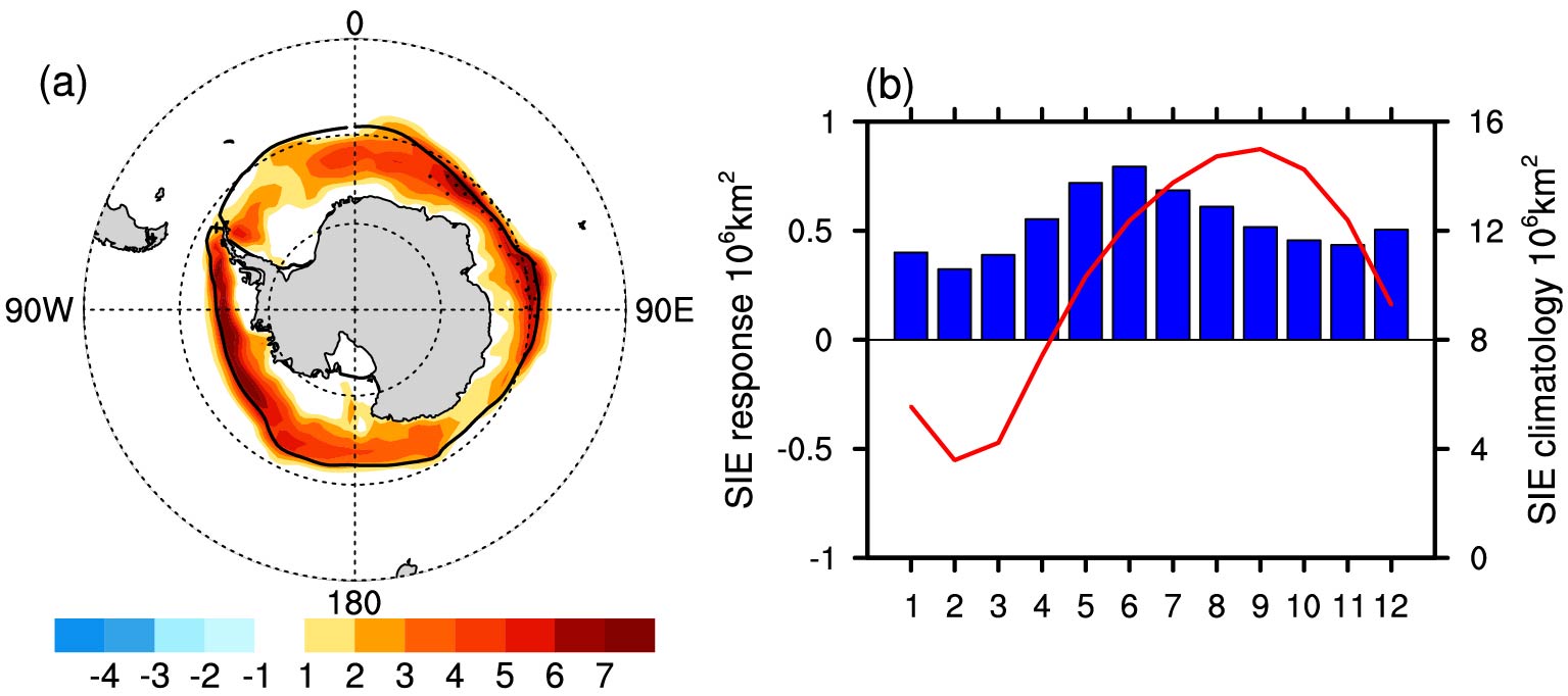 Figure1. Responses to ozone recovery of (a) annual-mean sea-ice fraction and (b) monthly-mean SIE in the SH. In (a), the bold black line denotes the annual-mean sea-ice edge, which is denoted by 15% sea-ice concentration, and the color interval is 1% (Student's t-test). Stippled areas are the regions where the differences are significant at the 95% confidence level. In (b), the left-hand vertical axis is the SIE response (blue bars) and the right-hand vertical axis is the absolute value of SIE (red line).
2
3.2. Responses of surface temperature and radiation budget to ozone recovery
Increasing sea-ice is associated with surface cooling of the Southern Ocean. Figure 2a shows the response of surface temperatures to ozone recovery. Significant cooling is found at SH middle and high latitudes, especially around the climatological sea-ice edge (bold black line). The largest cooling is about 1°C, located in the Amundsen-Bellingshausen Sea. Because sea surface temperatures (SSTs) at the sea-ice edge are just at the marginal of the freezing point, a 1°C decrease of SSTs can lead to sea-ice expansion.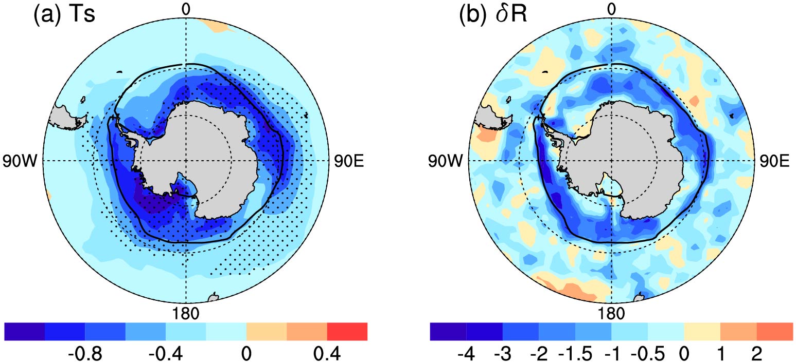 Figure2. Annual-mean responses of (a) surface temperatures and (b) surface radiation budget, including both SR and IR. Units: W m?2. Negative δR indicates a reduction in downward radiation absorbed by the surface. In (a), the color interval is 0.2 K, and dots mark the regions where responses have statistically significant levels higher than the 95 % confidence level (Student's t-test). In (b), the color bar is not linear. The black lines in both plots denote the annual-mean sea-ice edge.
The ocean surface cooling is associated with a reduction in the radiation budget at the surface. Figure 2b shows the annual-mean response of net surface radiation fluxes (δR) to ozone recovery, i.e., the sum of solar radiation (SR) absorbed by the surface and downward infrared radiation (IR). Negative δR indicates a decrease in radiation absorbed by the surface. In general, δR reduction is situated over SH middle and high latitudes. In particular, a band of relatively large δR reduction is right near the sea-ice edge. The largest δR reduction is greater than 3.0 W m?2. The question is how ozone recovery causes such a large reduction in the surface radiation budget, which is the major interest in this paper. We address this question as follows.
Using surface radiative kernels (Huang et al., 2017), we decompose δR into the direct radiative forcing of ozone recovery and other radiative effects such as changes in water vapor, clouds, and surface albedo. The instantaneous radiative forcing of ozone recovery is calculated with a rapid radiative transfer model (RRTM) (Mlawer et al., 1997). Clouds are prescribed in the RRTM using our simulation output. The annual-mean instantaneous radiative forcing at the surface due to ozone recovery is negative (Fig. 3a). This is because ozone recovery causes more ultraviolet radiation absorbed in the stratosphere, so that less SR reaches the surface. However, the largest negative value is only about 0.2 W m?2. The radiative forcing of water vapor changes is also negative (Fig. 3b). This is because atmospheric temperatures decrease as the surface cools. As a result, water vapor in the atmosphere is also decreased, and the radiative forcing of water vapor changes is negative. Increasing sea-ice also leads to a decrease in surface evaporation, which also contributes to the water vapor decrease. The largest negative forcing of water vapor is less than 0.5 W m?2. The sum of radiative forcing due to ozone recovery and the water vapor decrease is much weaker than that in Fig. 2a. These results suggest that the direct radiative forcing of ozone recovery and a decrease in water vapor are not the key factors causing surface cooling. Thus, there must be other factors responsible for the surface radiation reduction and surface cooling.
 Figure3. Annual-mean radiative forcings at the surface: (a) direct radiative forcing of ozone recovery; (b) radiative forcing of water vapor changes; (c) cloud radiative forcing (both, SR and IR); (d) surface albedo effect. Units: W m?2. Note that the color bar is not linear in scale. The black lines denote the annual-mean sea-ice edge.
Figure 3c shows much larger cloud-induced positive forcing at the surface, especially at the ice edge. The positive cloud forcing indicates that there must be decreases in cloud near the ice edge. Indeed, Fig. 4a shows a band of decreased cloud around the Antarctic, with the largest decrease greater than 2.5%. Meanwhile, clouds increase at SH midlatitudes, suggesting an equatorward shift of clouds. As we will address in section 3.4, the equatorward shift of clouds is because of the atmospheric thermal structure changes due to ozone recovery. Decreased cloud causes increased SR at the surface around the sea-ice edge Fig. 4b, and the largest increase in SR is greater than 4 W m?2. Decreased cloud also causes decreased downward IR at the surface (Fig. 4c), with the largest decrease being about 2 W m?2. Overall, cloud-induced radiative forcing at the surface is positive near the ice edge (Fig. 3c).
 Figure4. Annual-mean responses to ozone recovery: (a) cloud fraction; (b) cloud-induced SR; (c) cloud-induced downward IR. In (a), the color interval is 0.4%. In (b, c), the color interval is 0.5 W m?2. The black lines denote the annual-mean sea-ice edge. Regions with dots are the places where responses to ozone recovery is statistically significant at the 95% confidence level.
On the other hand, surface albedo causes large negative forcing (Fig. 3d). The largest negative value is greater than 4 W m?2. Such a large negative forcing is caused by increasing sea-ice, i.e., ice-albedo feedback. It suggests that the effect of ice-albedo plays the major role in causing the negative radiative forcing. Indeed, the spatial pattern of surface radiation reduction (Fig. 2b) largely resembles that of the ice-albedo forcing (Fig. 3d).
From Figs. 3 and 4, we can see that downward IR reduction due to cloud decreases and the ice-albedo effect due to increasing sea-ice are the two major negative forcings, while the direct radiative forcing of ozone recovery and the forcing of water vapor changes are weaker by one order of magnitude. Thus, surface cooling should be mainly caused by the two major negative forcings. For the two negative forcings, the albedo effect of increasing sea-ice can only enhance surface cooling, but not the forcing in initializing surface cooling. This is because increasing sea-ice is a result of surface cooling. Therefore, decrease downward IR due to cloud decreases should be the major forcing in initializing surface cooling, especially in the winter half of the year when cloud changes have little effect on SR over the Antarctic.
2
3.3. Seasonal variations
To address how cloud decreases and the associated decrease in downward IR cause surface cooling, we plot the seasonal variations of clouds and associated variables in responding to ozone recovery in Fig. 5. Clouds decrease in all months, with the largest decrease is in April and May (Fig. 5a). Note that the large cloud decrease in August cannot be a result of ozone recovery because no ultraviolet radiation is absorbed by ozone recovery during the polar night. Instead, it is more likely a result of large fluctuations in polar temperatures due to dynamic processes in the winter season. We will return to this point in section 3.4.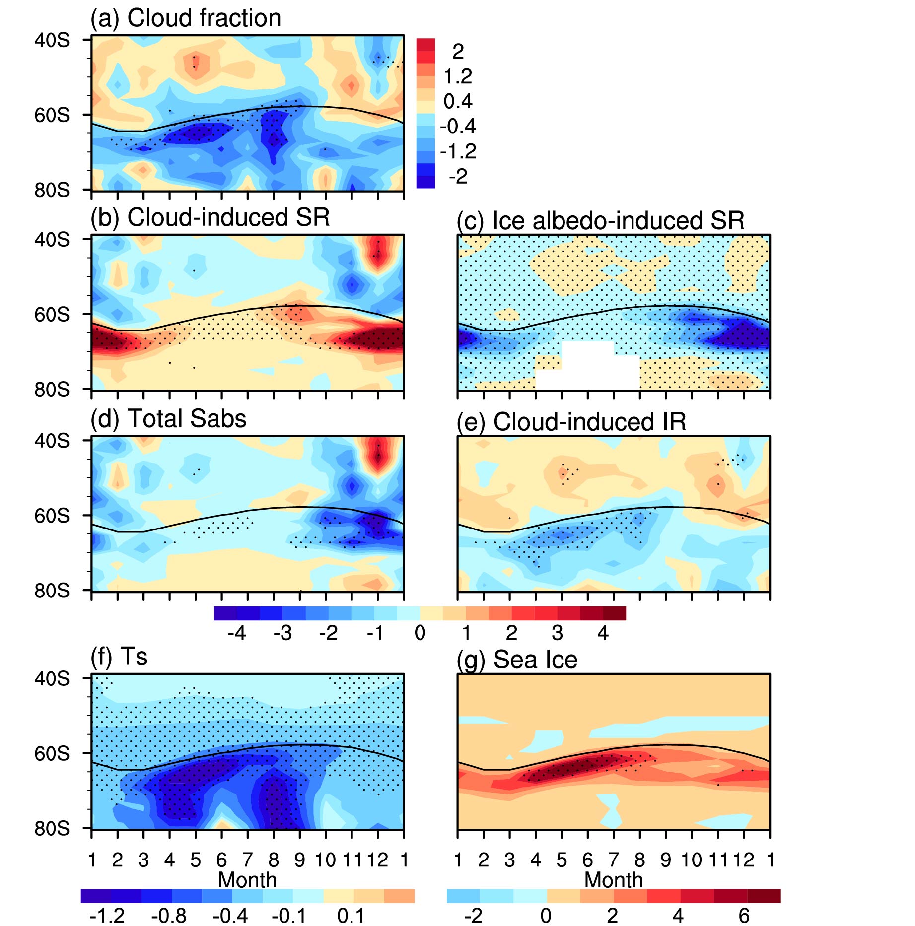 Figure5. Seasonal variations of zonal-mean responses to ozone recovery: (a) cloud fraction (%); (b) cloud-induced SR; (c) surface albedo effect; (d) net SR; (e) cloud-induced downward IR; (f) surface temperature; (g) sea-ice fraction. Black lines in all plots denote the sea-ice edge. In (a), the color interval is 0.4%. In (b–e), the color interval is 1 W m?2. The color interval in (f) is nonlinear, and the units are °C. The color interval in (g) is 1%. Regions with dots are the places where responses are statistically significant at the 95% confidence level.
Cloud decreases cause increasing SR at the surface mainly in austral summer (Fig. 5b). This is because summer is the polar-day season, and cloud decreases result in more SR increases than in other seasons. On the other hand, increasing sea-ice reflects SR back to space in austral summer, generating negative SR forcing at the surface (Fig. 5c). It is important to note that the negative forcing of the albedo effect is larger than the cloud-induced SR increase. Thus, SR absorbed by the surface is actually negative in austral summer (Fig. 5d). The largest negative value of SR absorbed by the surface is about 3 W m?2 in November-December.
Cloud-induced downward IR at the surface is negative in all months, with the largest values (about 2 W m?2) in austral autumn (Fig. 5e). Figure 5f shows that surface cooling exists all year round, with the largest cooling in March?June. Increasing sea-ice also lasts all year round, peaking in April?June (Fig. 5g). The seasonal variation of sea-ice is consistent with that of surface cooling.
The direct radiative forcing of ozone recovery at the surface and the radiative forcing of water vapor changes also show seasonal variations (Fig. 6). Ozone recovery has the largest negative forcing in October?January, with values less than 0.2 W m?2. The radiative forcing of water vapor changes is over March?July, with values less than 0.4 W m?2. As mentioned above, they are much weaker than the cloud-induced reduction of downward IR.
 Figure6. Seasonal variations of zonal-mean radiative forcing: (a) ozone recovery; (b) water vapor decreases. Units: W m?2. Black lines in both plots denote seasonal variations of the zonal-mean sea-ice edge.
The results in Fig. 5 reveal that cloud decreases at SH high latitudes are the major forcing in causing ocean surface cooling, and that austral autumn is the critical season when cloud-induced reduction of downward IR initiates surface cooling and increases in sea-ice. Cloud decreases mainly exist in austral autumn. In this season, the radiative effect of cloud decreases is mainly to reduce downward IR, while cloud-induced solar forcing is relatively weak because it is the season of sunset over the Antarctic. Thus, cloud decreases lead to surface cooling and increasing sea-ice. It is important to note that the sea-ice increase lasts all year round once it is initiated in austral autumn, and that its reflection of SR also lasts all year round. Although cloud decreases lead to large SR increases at the surface in austral summer, the increases of SR are offset by the reflection of increasing sea-ice. As a result, the ocean surface is also cooled in austral summer, and sea-ice also increases.
To summarize the seasonal variations, the largest decreases in cloud at SH high latitudes in austral autumn, due to ozone recovery, cause reduced downward IR and initialize surface cooling and increasing sea-ice. The increased sea-ice reflects SR and enhances surface cooling through the ice-albedo feedback process.
2
3.4. Cloud response to ozone recovery
The above results have shown how decreases in cloud at SH high latitudes cause surface cooling and increasing sea-ice. However, important questions remain to be answered, such as how ozone recovery leads to these cloud decreases, and why the largest decrease occurs in austral autumn. To answer these questions, we next analyze the relationship between cloud changes and ozone-induced atmospheric temperature changes. Figure 7 shows vertical cross-sections of zonal-mean temperature changes in response to ozone recovery in all four seasons. Ozone recovery leads to warming in the mid and high-latitude lower stratosphere, especially in the polar region. The strongest and significant warming is in December?January?February (DJF), with the largest value greater than 1.2°C (Fig. 7a). Although the warming in March?April?May (MAM) is relatively weak, it is statistically significant. In particular, the maximum warming region is over the ice edge (60°S to 70°S) (Fig. 7b). The warming in June?July?August (JJA) is less significant and cannot be explained by ozone recovery because JJA is the polar-night season (Fig. 7c). The insignificant warming is likely due to wave-driven dynamic heating, which has large fluctuations. The warming in September?October?November (SON) is large, but not statistically significant (Fig. 7d). It is probably because SON is the season when the Antarctic polar vortex breaks up and wave-driven dynamic heating causes large temperature fluctuations. Associated with the polar warming, the polar night jet shifts toward the equator in SON, DJF, and MAM (figures not shown), consistent with previous simulation results.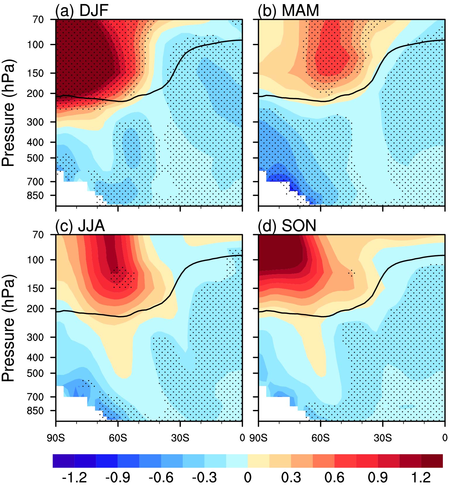 Figure7. Vertical cross section of zonal-mean temperature changes in response to ozone recovery: (a) DJF; (b) MAM; (c) JJA; (d) SON. Color interval: 0.15°C. The black lines denote the tropopause. Regions with dots are the places where responses are statistically significant at the 95% confidence level.
Figure 8 shows the zonal-mean cloud changes in response to ozone recovery. Significant cloud decreases are found in DJF and MAM (Fig. 8a and b). The common feature in the two seasons is that the largest and significant cloud decreases are around the tropopause. In particular, a band of cloud decreases is situated right over the ice edge and extends from the tropopause to the middle troposphere in MAM. In contrast, cloud decreases in JJA and SON are not statistically significant (Fig. 8c and 8d). This is consistent with the less significant temperature changes in JJA and SON. It has been suggested that the lower-stratospheric warming, due to ozone recovery, enhances static stability and reduces relative humidity in the upper troposphere and near the tropopause, and both contribute to cloud decreases (Jenkins, 1999; Yang et al., 2012; Xia et al., 2016, 2018). From Fig. 7, we can see that the contrast in temperature changes between the lower stratosphere and troposphere is larger in DJF and MAM than in JJA and SON. In DJF and MAM, warming in the lower stratosphere contrasts with cooling in the troposphere (Figs. 7a and b). However, the vertical temperature contrast in JJA and SON is weaker (Figs. 7c and d). Therefore, static stability is enhanced more by ozone recovery in DJF and MAM than in JJA and SON. In other words, convections near the tropopause is weakened more in DJF and MAM than in JJA and SON, leading to less cloud formation in DJF and MAM. The simulation results for clouds here are consistent with previous results in which significant increases in cirrus clouds were found to be associated with ozone depletion (Nowack et al., 2015).
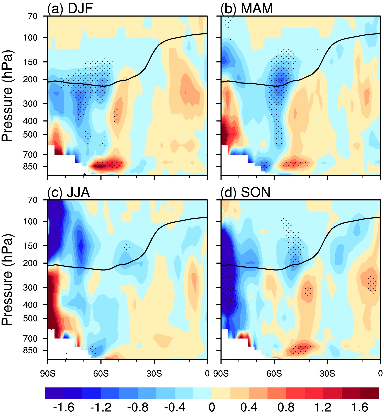 Figure8. Vertical cross section of zonal-mean cloud changes in response to ozone recovery: (a) DJF; (b) MAM; (c) JJA; (d) SON. Color interval; 0.2%. The black lines denote the tropopause. Regions with dots are the places where responses are statistically significant at the 95% confidence level.
To further confirm the relationship of changes between temperature and clouds, we regress the seasonal-mean area-weighted temperatures over 50°–90°S and between 250 and 150 hPa onto the zonal-mean cloud fraction, using the last 40 years' simulation output (Fig. 9). It is found that high clouds over the sea-ice edge between 60°–70°S are closely related to the temperature changes around the tropopause, except for DJF. The results in Fig. 9 indicate that high clouds decrease as temperatures near the tropopause increase. It is important to note that the regression coefficient reaches about 1.4% K?1 over the ice edge in MAM much larger than the values of 0.8% K?1 in DJF. Thus, cloud fraction is more sensitive to tropopause temperature changes in MAM than in DJF. Although high clouds in JJA and SON also have close correlations with tropopause temperatures, the responses of high clouds to ozone recovery are not significant, because tropopause temperature changes are not significant in the two seasons.
 Figure9. Regression of seasonal-mean area-weighted temperature over 50°–90°S and between 250 and 150 hPa onto the zonal-mean cloud fraction: (a) DJF; (b) MAM; (c) JJA; (d) SON. The units are % K?1. Regions with dots are the places where responses are statistically significant at the 95% confidence level.
It is worth pointing out that, in this study, the atmospheric GCM is coupled only with a slab ocean to distinguish ozone-induced cloud radiative effects on sea-ice. Thus, our simulation result has its own limitations because ocean heat transports and dynamic sea-ice are excluded. As demonstrated in previous AOGCM studies (Sigmond and Fyfe, 2010; Bitz and Polvani, 2012; Smith et al., 2012), ozone-induced changes in atmospheric and oceanic circulations significantly alter ocean heat transports and sea-ice dynamics, and consequently impact SSTs and Antarctic sea-ice. Thus, these dynamic processes, together with the cloud radiative effects, all have important contributions to increasing Antarctic sea-ice. In fact, ozone-induced cloud radiative effects have been included in previous AOGCM simulations. It is important to diagnose the respective contributions of cloud radiative effects and dynamic processes in AOGCM simulations in future studies.
Another issue that needs to be further addressed is the sea-ice feedback to cloud formation. In the present study, we have emphasized the importance of ice-albedo feedback to the surface radiation budget. Increasing sea-ice will also reduce water evaporation from the ocean surface, and lower the water vapor content in the atmosphere. Consequently, it will reduce cloud formation. This requires diagnosis of the feedback of sea-ice to cloud formation in future studies.
Acknowledgements. This research is supported by the National Key R&D Program of China (2018YFA0605901). Y. XIA and Y. Y. HU are supported by the National Natural Science Foundation of China (NSFC) (Grant Nos. 41530423 and 41761144072). Y. XIA is supported by the China Postdoctoral Science Foundation funded project (Grant No. 2018M630027). Y. HUANG is supported by the Discovery Program of the Natural Sciences and Engineering Council of Canada (Grant No. RGPIN 418305-13) and the Team Research Project Program of the Fonds de Recherché Nature et Technologies of Quebec (Grant No. PR-190145). J. P. LIU is supported by the Climate Observation and Earth System Science Divisions, Climate Program Office, NOAA, U.S. Department of Commerce (Grant Nos. NA15OAR4310163 and NA14OAR4310216). J. T. LIN is supported by the NSFC (Grant No. 41775115) and the 973 program (Grant No. 2014CB441303).
Open Access This article is distributed under the terms of the Creative Commons Attribution 4.0 International License (http://creativecommons.org/licenses/by/4.0/), which permits unrestricted use, distribution, and reproduction in any medium, provided you give appropriate credit to the original author(s) and the source, provide a link to the Creative Commons license, and indicate if changes were made.
