Hui-Juan Wang^1,2, Zun-Yan Di¹, Zhi-Gang Wang^,11Department of Physics, North China Electric Power University, Baoding 071003, China
²School of Nuclear Sicence and Engineering, North China Electric Power University, Beijing 102206, China

Received:2020-07-30Revised:2020-09-28Accepted:2020-11-4Online:2021-02-04


Abstract
We construct both the scalar-diquark-scalar-diquark-antiquark type and axialvector-diquark-axialvector-diquark-antiquark type interpolating currents to study the charmed pentaquark states ${susc}\bar{u}$ with ${J}^{P}={\tfrac{1}{2}}^{\pm }$. We employ the QCD sum rules to investigate the masses and pole residues of the charmed pentaquark states by taking into account the vacuum condensates up to dimension 13 in the operator product expansion. Our calculation results indicate that the scalar-diquark-scalar-diquark-antiquark type and axialvector-diquark-axialvector-diquark-antiquark type charmed pentaquark states ${susc}\bar{u}$ with ${J}^{P}={\tfrac{1}{2}}^{-}$ can be possible candidates of the excited Ω_c states observed in the LHCb collaboration.
Keywords： charmed baryon states;charmed pentaquark states;QCD sum rules


PDF (1027KB)MetadataMetricsRelated articlesExportEndNote|Ris|BibtexFavorite
Cite this article
Hui-Juan Wang, Zun-Yan Di, Zhi-Gang Wang. Analysis of the excited Ω_c states as the $\tfrac{1}{2}$^± pentaquark states with QCD sum rules. Communications in Theoretical Physics, 2021, 73(3): 035201- doi:10.1088/1572-9494/abc7b1

1. Introduction

In 2017, five new narrow excited Ω_c states named Ω_c(3000), Ω_c(3050), Ω_c(3066), Ω_c(3090) and Ω_c(3119) were observed in the LHCb collaboration [1]. These new observed hadrons were reported to be the excited states of Ω_c which is composed of one c quark and two s quarks. The decay widths of these states were also measured, which were only a few MeV. However, the quantum numbers of theses excited states are not confirmed until now.

The above discovery inspired a large amount of theoretical studies of these excited Ω_c states with different asssumptions of their structures. Conventionally, these states were interpreted in three-quark frames [2–13] and assigned as the orbitally or radially excited states of the Ω_c baryons. In [9], the authors employed the QCD sum rules on the light-cone to study the decay properties of Ω_c baryons and assigned Ω_c(3000), Ω_c(3050) and Ω_c(3119) to be $\left(1P,{\tfrac{1}{2}}^{-}\right)$, $\left(1P,{\tfrac{3}{2}}^{-}\right)$ and $\left(2S,{\tfrac{3}{2}}^{+}\right)$, respectively. In [10], the authors assigned Ω_c(3066) and Ω_c(3119) as the 2S states, and used the QCD sum rules to calculate the masses of these states. In [11], the authors employed the ³p₀ model to study the decay widths of the charmed baryons and interpreted Ω_c(3066) and Ω_c(3090) to be 1P-wave with ${J}^{P}={\tfrac{3}{2}}^{-}$ and ${\tfrac{5}{2}}^{-}$, respectively. The possibility of the assignment of the 1D-wave states were also discussed in [11]. In [12], we assigned Ω_c(3000) and Ω_c(3119) to be $\left(1P,{\tfrac{1}{2}}^{-}\right)$ and $\left(2S,{\tfrac{3}{2}}^{+}\right)$, respectively, and assigned Ω_c(3090) to be $\left(1P,{\tfrac{3}{2}}^{-}\right)$ or $(2S,{\tfrac{1}{2}}^{+})$. In [13], our calculation predicted Ω_c(3000), Ω_c(3050), Ω_c(3066), Ω_c(3090) and Ω_c(3119) to be the P-wave baryon states with ${J}^{P}={\tfrac{1}{2}}^{-}$, ${\tfrac{1}{2}}^{-}$, ${\tfrac{3}{2}}^{-}$, ${\tfrac{3}{2}}^{-}$ and ${\tfrac{5}{2}}^{-}$, respectively.

In 2015, the LHCb reported the exotic structure P_c(4450) which also has a narrow decay width of 39±5±19 MeV [14]. In [15], the analysis of the low-lying pentaquark states with S=−3 and negative parity indicated that baryon excitation by pulling out a $q\overline{q}$ pair may need less energy than by the tranditional orbital excitation. The ground states of Ω_c are Ω_c(2695) and Ω_c(2770) with spin-parity ${J}^{P}={\tfrac{1}{2}}^{+}$ and ${\tfrac{3}{2}}^{+}$ which had been observed experimentally. The mass gaps between the excited Ω_c states and the ground states are 230–424 MeV, which are large enough to excite a light quark-antiquark pair. It means these excited states can be the multiquark candidates.

Kim et al proposed Ω_c(3050) and Ω_c(3119) to be exotic pentaquarks with ${J}^{P}={\tfrac{1}{2}}^{+}$ and ${\tfrac{3}{2}}^{+}$, respectively, in the chiral quark-soliton model. The calculation of the strong decays of Ω_c(3050) and Ω_c(3119) supported the assignment and naturally explained the LHCb obsevation that Ω_c(3050) and Ω_c(3119) have anomalously small widths [16]. In [17], the investigation found that the pentaquark configurations take sizable probabilities in these Ω_c baryons. Yang and Ping studied both the three-quark system with ssc and the five-quark system with ${sscu}\overline{u}$ and ${sscd}\overline{d}$ by performing the dynamical calculation of Ω_c in the framework of the chiral quark model [18]. Those excited states were also considered as candidates of molecular states [19–21]. In [22], we designed these excited states as axialvector-diquark-scalar-diquark-antiquark type charmed pentaquark states with ${J}^{P}={\tfrac{3}{2}}^{\pm }$.

In our previous work, we have ever assigned the five Ω_c states as conventional three-quark baryon states [12, 13] and axialvector-diquark-scalar-diquark-antiquark type charmed pentaquark states [22]. A hadron could have a lot of Fock states, which can couple to different interpolating currents with certain quantum numbers. Up to now, the mass spectrums of these Ω_c states were not determined, we can construct different three-quark and pentaquark interpolating currents to investigate the inner structures of these hadrons. In the present work, in order to explore the possible interpretation of pentaquark states for these Ω_c states, we construct both the scalar-diquark-scalar-diquark-antiquark type and axialvector-diquark-axialvector-diquark-antiquark type interpolating currents to study the charmed pentaquark states ${susc}\bar{u}$ with ${J}^{P}={\tfrac{1}{2}}^{\pm }$. By considering the vacuum condensates up to dimension 13 we investigated the masses and pole residues of the charmed pentaquark states through the QCD sum rules. Comparing the results with the measurement of LHCb, it is found that the scalar-diquark-scalar-diquark-antiquark type and axialvector-diquark-axialvector-diquark-antiquark type charmed pentaquark states ${susc}\bar{u}$ with ${J}^{P}={\tfrac{1}{2}}^{-}$ can be possible candidates of the excited Ω_c states observed in the LHCb collaboration.

2. QCD sum rules for the ${\tfrac{1}{2}}^{\pm }$ charmed pentaquark states

The two-point correlation function in QCD rum rules is written as follow(1)$\begin{eqnarray}{\rm{\Pi }}(p)={\rm{i}}\int {{\rm{d}}}^{4}x{{\rm{e}}}^{{\rm{i}}p\cdot x}\left\langle 0| T\left\{J(x)\bar{J}(0)\right\}| 0\right\rangle ,\end{eqnarray}$where(2)$\begin{eqnarray}\begin{array}{rcl}J(x) & = & {J}_{1}(x),{J}_{2}(x),\\ {J}_{1}(x) & = & {\varepsilon }^{{ila}}{\varepsilon }^{{ijk}}{\varepsilon }^{{lmn}}{s}_{j}^{{\rm{T}}}(x)C{\gamma }_{5}{u}_{k}(x){s}_{m}^{{\rm{T}}}(x)C{\gamma }_{5}{c}_{n}(x)C{\bar{u}}_{a}^{{\rm{T}}}(x),\\ {J}_{2}(x) & = & {\varepsilon }^{{ila}}{\varepsilon }^{{ijk}}{\varepsilon }^{{lmn}}{s}_{j}^{{\rm{T}}}(x)C{\gamma }_{\mu }{u}_{k}(x){s}_{m}^{{\rm{T}}}(x)C{\gamma }^{\mu }{c}_{n}(x)C{\bar{u}}_{a}^{{\rm{T}}}(x),\end{array}\end{eqnarray}$i, j, k, l, m, n and a are color indices, C is the charge conjugation matrix. In this work, we construct the scalar-diquark-scalar-diquark-antiquark type and axialvector-diquark-axialvector-diquark-antiquark type interpolating currents to study the charmed pentaquark states ${susc}\bar{u}$ with ${J}^{P}={\tfrac{1}{2}}^{\pm }$.

At the phenomenological side, a complete set of intermediate pentaquark states with the same quantum numbers as the current operators J(x) and iγ₅J(x) are inserted into the correlation functions Π(p) to obtain the hadronic representation [23]. The result is obtained as follow after isolating the lowest states with ${J}^{P}={\tfrac{1}{2}}^{\pm }$.(3)$\begin{eqnarray}{\rm{\Pi }}(p)={\lambda }_{-}^{2}\displaystyle \frac{{/}\!\!\!{p}+{M}_{-}}{{M}_{-}^{2}-{p}^{2}}+{\lambda }_{+}^{2}{\displaystyle \frac{{/}\!\!\!{p}-{M}_{+}}{{M}_{+}^{2}-{p}^{2}}}_{}+\cdots ,\end{eqnarray}$where M_± and λ_± are the masses and the pole residues of the lowest states corresponding to ${J}^{P}={\tfrac{1}{2}}^{\pm }$, respectively.

The currents J(0) couple potentially to the charmed pentaquark states with ${J}^{P}={\tfrac{1}{2}}^{\pm }$ [24](4)$\begin{eqnarray}\begin{array}{rcl}\langle 0| J(0)| {P}_{-}(p)\rangle & = & {\lambda }_{-}{U}^{-}(p,s),\\ \langle 0| J(0)| {P}_{+}(p)\rangle & = & {\lambda }_{+}{\rm{i}}{\gamma }_{5}{U}^{+}(p,s).\end{array}\end{eqnarray}$

Based on dispersion relation, we can obtain the hadronic spectral densities at the phenomenological side(5)$\begin{eqnarray}\begin{array}{rcl}\displaystyle \frac{\mathrm{Im}{\rm{\Pi }}(s)}{\pi } & = & {/}\!\!\!{p}\left[{\lambda }_{-}^{2}\delta \left(s-{M}_{-}^{2}\right)+{\lambda }_{+}^{2}\delta \left(s-{M}_{+}^{2}\right)\right]\\ & & +\left[{M}_{-}{\lambda }_{-}^{2}\delta \left(s-{M}_{-}^{2}\right)-{M}_{+}{\lambda }_{+}^{2}\delta \left(s-{M}_{+}^{2}\right)\right]\\ & = & {/}\!\!\!{p}\,{\rho }_{H}^{1}(s)+{\rho }_{H}^{0}(s).\end{array}\end{eqnarray}$

We can obtain the QCD sum rules at the hadron side by introducing the weight function $\exp \left(-\tfrac{s}{{T}^{2}}\right)$,(6)$\begin{eqnarray}\begin{array}{l}{\displaystyle \int }_{{m}_{c}^{2}}^{{s}_{0}}{\rm{d}}s\left[\sqrt{s}{\rho }_{H}^{1}(s)\mp {\rho }_{H}^{0}(s)\right]\exp \left(-\displaystyle \frac{s}{{T}^{2}}\right)\\ \quad =\,2{M}_{\pm }{\lambda }_{\pm }^{2}\exp \left(-\displaystyle \frac{{M}_{\pm }^{2}}{{T}^{2}}\right),\end{array}\end{eqnarray}$where the subscript H denotes the hadron side, s₀ is the continuum threshold parameter and T² is the Borel parameter [24]. According to equations (5) and (6), we can separate the negative parity state from the positive parity state clearly.

We briefly outline the operator product expansion for the correlation functions Π_1,2(p). Using Wick theorem we contract the s, u and c quark fields in the correlation function Π_1,2(p) and obtain the results as follow:(7)$\begin{eqnarray}\begin{array}{rcl}{{\rm{\Pi }}}_{1}(p) & = & {\rm{i}}\,{\varepsilon }^{{ila}}{\varepsilon }^{{ijk}}{\varepsilon }^{{lmn}}{\varepsilon }^{{i}^{{\prime} }{l}^{{\prime} }{a}^{{\prime} }}{\varepsilon }^{{i}^{{\prime} }{j}^{{\prime} }{k}^{{\prime} }}{\varepsilon }^{{l}^{{\prime} }{m}^{{\prime} }{n}^{{\prime} }}\displaystyle \int {{\rm{d}}}^{4}x{{\rm{e}}}^{{\rm{i}}p\cdot x}\\ & & \left\{-\mathrm{Tr}\left[{\gamma }_{5}{U}_{{{kk}}^{{\prime} }}(x){\gamma }_{5}{{CS}}_{{{jj}}^{{\prime} }}^{{\rm{T}}}(x)C\right]\right.\\ & & \times \mathrm{Tr}\left[{\gamma }_{5}{C}_{{{nn}}^{{\prime} }}(x){\gamma }_{5}{{CS}}_{{{mm}}^{{\prime} }}^{{\rm{T}}}(x)C\right]\,{{CU}}_{{a}^{{\prime} }a}^{{\rm{T}}}(-x)C\\ & & +\mathrm{Tr}\left[{\gamma }_{5}{U}_{{{kk}}^{{\prime} }}(x){\gamma }_{5}{{CS}}_{{{mj}}^{{\prime} }}^{{\rm{T}}}(x)C{\gamma }_{5}{C}_{{{nn}}^{{\prime} }}(x)\right.\\ & & \times \left.\left.{\gamma }_{5}{{CS}}_{{{jm}}^{{\prime} }}^{{\rm{T}}}(x)C\right]\,{{CU}}_{{a}^{{\prime} }a}^{{\rm{T}}}(-x)C\right\},\end{array}\end{eqnarray}$(8)$\begin{eqnarray}\begin{array}{rcl}{{\rm{\Pi }}}_{2}(p) & = & {\rm{i}}\,{\varepsilon }^{{ila}}{\varepsilon }^{{ijk}}{\varepsilon }^{{lmn}}{\varepsilon }^{{i}^{{\prime} }{l}^{{\prime} }{a}^{{\prime} }}{\varepsilon }^{{i}^{{\prime} }{j}^{{\prime} }{k}^{{\prime} }}{\varepsilon }^{{l}^{{\prime} }{m}^{{\prime} }{n}^{{\prime} }}\displaystyle \int {{\rm{d}}}^{4}x{{\rm{e}}}^{{\rm{i}}p\cdot x}\\ & & \left\{-\mathrm{Tr}\left[{\gamma }_{\mu }{U}_{{{kk}}^{{\prime} }}(x){\gamma }_{\nu }{{CS}}_{{{jj}}^{{\prime} }}^{{\rm{T}}}(x)C\right]\right.\\ & & \times \mathrm{Tr}\left[{\gamma }^{\mu }{C}_{{{nn}}^{{\prime} }}(x){\gamma }^{\nu }{{CS}}_{{{mm}}^{{\prime} }}^{{\rm{T}}}(x)C\right]\,{{CU}}_{{a}^{{\prime} }a}^{{\rm{T}}}(-x)C\\ & & +\mathrm{Tr}\left[{\gamma }_{\mu }{U}_{{{kk}}^{{\prime} }}(x){\gamma }_{\nu }{{CS}}_{{{mj}}^{{\prime} }}^{{\rm{T}}}(x)C{\gamma }^{\mu }{C}_{{{nn}}^{{\prime} }}(x)\right.\\ & & \left.\left.\times {\gamma }^{\nu }{{CS}}_{{{jm}}^{{\prime} }}^{{\rm{T}}}(x)C\right]\,{{CU}}_{{a}^{{\prime} }a}^{{\rm{T}}}(-x)C\right\},\end{array}\end{eqnarray}$where U_ij(x), S_ij(x) and C_ij(x) are the full u, s and c quark propagators, respectively [23](9)$\begin{eqnarray}\begin{array}{rcl}{U}_{{ij}}(x) & = & \displaystyle \frac{{\rm{i}}{\delta }_{{ij}}{/}\!\!\!{x}}{2{\pi }^{2}{x}^{4}}-\displaystyle \frac{{\delta }_{{ij}}\langle \bar{q}q\rangle }{12}-\displaystyle \frac{{\delta }_{{ij}}{x}^{2}\langle \bar{q}{g}_{s}\sigma {Gq}\rangle }{192}\\ & & -\displaystyle \frac{{\rm{i}}{g}_{s}{G}_{\alpha \beta }^{a}{t}_{{ij}}^{a}({/}\!\!\!{x}{\sigma }^{\alpha \beta }+{\sigma }^{\alpha \beta }{/}\!\!\!{x})}{32{\pi }^{2}{x}^{2}}\\ & & -\displaystyle \frac{1}{8}\langle {\bar{q}}_{j}{\sigma }^{\mu \nu }{q}_{i}\rangle {\sigma }_{\mu \nu }+\cdots ,\end{array}\end{eqnarray}$(10)$\begin{eqnarray}\begin{array}{rcl}{S}_{{ij}}(x) & = & \displaystyle \frac{{\rm{i}}{\delta }_{{ij}}{/}\!\!\!{x}}{2{\pi }^{2}{x}^{4}}-\displaystyle \frac{{\delta }_{{ij}}{m}_{s}}{4{\pi }^{2}{x}^{2}}-\displaystyle \frac{{\delta }_{{ij}}\langle \bar{s}s\rangle }{12}\\ & & +\displaystyle \frac{{\rm{i}}{\delta }_{{ij}}{/}\!\!\!{x}{m}_{s}\langle \bar{s}s\rangle }{48}-\displaystyle \frac{{\delta }_{{ij}}{x}^{2}\langle \bar{s}{g}_{s}\sigma {Gs}\rangle }{192}\\ & & +\displaystyle \frac{{\rm{i}}{\delta }_{{ij}}{x}^{2}{/}\!\!\!{x}{m}_{s}\langle \bar{s}{g}_{s}\sigma {Gs}\rangle }{1152}-\displaystyle \frac{{\rm{i}}{g}_{s}{G}_{\alpha \beta }^{a}{t}_{{ij}}^{a}({/}\!\!\!{x}{\sigma }^{\alpha \beta }+{\sigma }^{\alpha \beta }{/}\!\!\!{x})}{32{\pi }^{2}{x}^{2}}\\ & & -\displaystyle \frac{1}{8}\langle {\bar{s}}_{j}{\sigma }^{\mu \nu }{s}_{i}\rangle {\sigma }_{\mu \nu }+\cdots ,\end{array}\end{eqnarray}$(11)$\begin{eqnarray}\begin{array}{rcl}{C}_{{ij}}(x) & = & \displaystyle \frac{{\rm{i}}}{{\left(2\pi \right)}^{4}}\displaystyle \int {{\rm{d}}}^{4}k{{\rm{e}}}^{-{\rm{i}}k\cdot x}\left\{\displaystyle \frac{{\delta }_{{ij}}}{{/}\!\!\!{k}-{m}_{c}}\right.\\ & & \left.-\displaystyle \frac{{g}_{s}{G}_{\alpha \beta }^{n}{t}_{{ij}}^{n}}{4}\displaystyle \frac{{\sigma }^{\alpha \beta }({/}\!\!\!{k}+{m}_{c})+({/}\!\!\!{k}+{m}_{c}){\sigma }^{\alpha \beta }}{{\left({k}^{2}-{m}_{c}^{2}\right)}^{2}}+\cdots \right\},\end{array}\,\end{eqnarray}$here, ${t}^{n}=\tfrac{{\lambda }^{n}}{2}$, λⁿ is the Gell-Mann matrix [23]. In equations (9) and (10), we retain the terms $\langle {\bar{q}}_{j}{\sigma }_{\mu \nu }{q}_{i}\rangle $ and $\langle {\bar{s}}_{j}{\sigma }_{\mu \nu }{s}_{i}\rangle $ respectively, which come from the Fierz re-ordering of $\langle {q}_{i}{\bar{q}}_{j}\rangle $ and $\langle {s}_{i}{\bar{s}}_{j}\rangle $ to absorb the gluons so as to extract the mixed condensate $\langle \bar{q}{g}_{s}\sigma {Gq}\rangle $ and $\langle \bar{s}{g}_{s}\sigma {Gs}\rangle $. The terms $-\tfrac{1}{8}\langle {\bar{q}}_{j}{\sigma }^{\mu \nu }{q}_{i}\rangle {\sigma }_{\mu \nu }$ and $-\tfrac{1}{8}\langle {\bar{s}}_{j}{\sigma }^{\mu \nu }{s}_{i}\rangle {\sigma }_{\mu \nu }$ were introduced in [25–27]. We can get the correlation function Π(p²) at the quark level by performing integral operation in both the coordinate space and the momentum space. According to the dispersion relation, the QCD spectral densities can be obtained as follow(12)$\begin{eqnarray}\displaystyle \frac{\mathrm{Im}{\rm{\Pi }}(s)}{\pi }={/}\!\!\!{p}\,{\rho }_{\mathrm{QCD}}^{1}(s)+{\rho }_{\mathrm{QCD}}^{0}(s).\end{eqnarray}$

After obtaining the QCD spectral densities ${\rho }_{\mathrm{QCD}}^{1}(s)$ and ${\rho }_{\mathrm{QCD}}^{0}(s)$, we take the quark-hadron duality below the continuum threshold parameter s₀ and introduce the weight function $\exp \left(-\tfrac{s}{{T}^{2}}\right)$ to obtain the QCD sum rules:(13)$\begin{eqnarray}\begin{array}{l}{\displaystyle \int }_{{m}_{c}^{2}}^{{s}_{0}}{\rm{d}}s\left[\sqrt{s}{\rho }_{H}^{1}(s)\pm {\rho }_{H}^{0}(s)\right]\exp \left(-\displaystyle \frac{s}{{T}^{2}}\right)\\ \quad =\,{\displaystyle \int }_{{m}_{c}^{2}}^{{s}_{0}}{\rm{d}}s\left[\sqrt{s}{\rho }_{\mathrm{QCD}}^{1}(s)\pm {\rho }_{\mathrm{QCD}}^{0}(s)\right]\exp \left(-\displaystyle \frac{s}{{T}^{2}}\right).\end{array}\end{eqnarray}$

The QCD sum rules can be rewritten clearly as follow(14)$\begin{eqnarray}\begin{array}{l}2{M}_{\pm }{\lambda }_{\pm }^{2}\exp \left(-\displaystyle \frac{{M}_{\pm }^{2}}{{T}^{2}}\right)\\ \quad =\,{\displaystyle \int }_{{m}_{c}^{2}}^{{s}_{0}}{\rm{d}}s\left[\sqrt{s}{\rho }_{\mathrm{QCD}}^{1}(s)\mp {\rho }_{\mathrm{QCD}}^{0}(s)\right]\exp \left(-\displaystyle \frac{s}{{T}^{2}}\right).\end{array}\end{eqnarray}$

We derive equation (14) with respect to $\tau =\tfrac{1}{{T}^{2}}$, then eliminate the pole residues λ_± and obtain the QCD sum rules for the masses of the charmed pentaquark states(15)$\begin{eqnarray}{M}_{\pm }^{2}=\displaystyle \frac{-\tfrac{{\rm{d}}}{{\rm{d}}\tau }{\int }_{{m}_{c}^{2}}^{{s}_{0}}{\rm{d}}s\left[\sqrt{s}{\rho }_{\mathrm{QCD}}^{1}(s)\mp {\rho }_{\mathrm{QCD}}^{0}(s)\right]\exp \left(-s\tau \right)}{{\int }_{{m}_{c}^{2}}^{{s}_{0}}{\rm{d}}s\left[\sqrt{s}{\rho }_{\mathrm{QCD}}^{1}(s)\mp {\rho }_{\mathrm{QCD}}^{0}(s)\right]\exp \left(-s\tau \right)},\end{eqnarray}$where M_± are the masses of the charmed pentaquark states with ${J}^{P}={\tfrac{1}{2}}^{\pm }$. Once the masses M_± are obtained, we can take them as input parameters and obtain the pole residues from the QCD sum rules in equation (14).

3. Numerical results and discussions

In our calculation, the vacuum condensates values are taken as ${m}_{0}^{2}=(0.8\pm 0.1){\mathrm{GeV}}^{2}$, $\langle \bar{s}s\rangle =(0.8\pm 0.1)\langle \bar{q}q\rangle $, $\langle \bar{q}q\rangle \,=-{(0.24\pm 0.01\mathrm{GeV})}^{3}$, $\langle \bar{q}{g}_{s}\sigma {Gq}\rangle ={m}_{0}^{2}\langle \bar{q}q\rangle $, $\langle \bar{s}{g}_{s}\sigma {Gs}\rangle \,={m}_{0}^{2}\langle \bar{s}s\rangle $, $\left\langle \tfrac{{\alpha }_{s}{GG}}{\pi }\right\rangle ={(0.33\mathrm{GeV})}^{4}$ at the energy scale μ=1 GeV [23], The quark condensate and the mixed quark condensate evolve with the renormalization group equation [28, 29](16)$\begin{eqnarray}\begin{array}{rcl}\langle \bar{q}q\rangle (\mu ) & = & \langle \bar{q}q\rangle (1\mathrm{GeV}){\left[\displaystyle \frac{{\alpha }_{s}(1\mathrm{GeV})}{{\alpha }_{s}(\mu )}\right]}^{\tfrac{12}{33-2{n}_{f}}},\\ \langle \bar{s}s\rangle (\mu ) & = & \langle \bar{s}s\rangle (1\mathrm{GeV}){\left[\displaystyle \frac{{\alpha }_{s}(1\mathrm{GeV})}{{\alpha }_{s}(\mu )}\right]}^{\tfrac{12}{33-{n}_{f}}},\\ \langle \bar{q}{g}_{s}\sigma {Gq}\rangle (\mu ) & = & \langle \bar{q}{g}_{s}\sigma {Gq}\rangle (1\mathrm{GeV}){\left[\displaystyle \frac{{\alpha }_{s}(1\mathrm{GeV})}{{\alpha }_{s}(\mu )}\right]}^{\tfrac{2}{33-2{n}_{f}}},\\ \langle \bar{s}{g}_{s}\sigma {Gs}\rangle (\mu ) & = & \langle \bar{s}{g}_{s}\sigma {Gs}\rangle (1\mathrm{GeV}){\left[\displaystyle \frac{{\alpha }_{s}(1\mathrm{GeV})}{{\alpha }_{s}(\mu )}\right]}^{\tfrac{2}{33-2{n}_{f}}},\end{array}\end{eqnarray}$here, we choose the $\overline{\mathrm{MS}}$ masses m_c(m_c)=(1.28±0.03) GeV and ${m}_{s}(\mu =2\,\mathrm{GeV})={0.096}_{-0.004}^{+0.008}\,\mathrm{GeV}$ from the Particle Data Group [30]. Furthermore, we take into account the energy-scale dependence of the $\overline{\mathrm{MS}}$ masses from the renormalization group equation(17)$\begin{eqnarray}\begin{array}{rcl}{m}_{c}(\mu ) & = & {m}_{c}({m}_{c}){\left[\displaystyle \frac{{\alpha }_{s}(\mu )}{{\alpha }_{s}({m}_{c})}\right]}^{\tfrac{12}{33-2{n}_{f}}},\\ {m}_{s}(\mu ) & = & {m}_{s}(2\mathrm{GeV}){\left[\displaystyle \frac{{\alpha }_{s}(\mu )}{{\alpha }_{s}(2\mathrm{GeV})}\right]}^{\tfrac{12}{33-2{n}_{f}}},\\ {\alpha }_{s}(\mu ) & = & \displaystyle \frac{1}{{b}_{0}t}\left[1-\displaystyle \frac{{b}_{1}}{{b}_{0}^{2}}\displaystyle \frac{\mathrm{log}t}{t}\right.\\ & & \left.+\displaystyle \frac{{b}_{1}^{2}({\mathrm{log}}^{2}t-\mathrm{log}t-1)+{b}_{0}{b}_{2}}{{b}_{0}^{4}{t}^{2}}\right],\end{array}\end{eqnarray}$where $t=\mathrm{log}\tfrac{{\mu }^{2}}{{{\rm{\Lambda }}}^{2}}$, ${b}_{0}=\tfrac{33-2{n}_{f}}{12\pi }$, ${b}_{1}=\tfrac{153-19{n}_{f}}{24{\pi }^{2}}$, ${b}_{2}\,=\tfrac{2857-\tfrac{5033}{9}{n}_{f}+\tfrac{325}{27}{n}_{f}^{2}}{128{\pi }^{3}}$, Λ=213 MeV, 296 MeV and 339 MeV for the flavors n_f=5, 4 and 3, respectively [30–32]. Here, we evolve all the input parameters at the QCD side to the optimal energy scales μ with n_f=4 to extract the pentaquark masses.

We have ever discussed how to choose the optimal energy scale and suggested an energy scale formula $\sqrt{{M}_{P}^{2}-{(2{{\mathbb{M}}}_{Q})}^{2}}$ to study hidden charmed (bottom) tetraquark states, pentaquark states and molecular states in the QCD rum rules in details [24–27]. The effective Q-quark masses ${{\mathbb{M}}}_{Q}$ embody the net effect of the complex dynamics and have universal values [24–27]. In this paper, we rewrite the energy scale formula as $\mu =\sqrt{{M}_{P}^{2}-{{\mathbb{M}}}_{c}^{2}}$, because there exists only one c quark, and take the effective c-quark mass ${{\mathbb{M}}}_{c}=1.82\,\mathrm{GeV}$ [33].

Here, we study the charmed pentaquark states with three types of energy scale parameters. Firstly, we evolve the input parameters to the energy scale $\mu =\sqrt{{M}_{P}^{2}-{{\mathbb{M}}}_{c}^{2}}$ to extract the masses M_P. Then, we evolve the input parameters to the energy scale μ=1 GeV to extract the masses M_P [34, 35]. Finally, we evolve the input parameters except for m_c(m_c) to the energy scale μ=1GeV to extract the masses M_P which is denoted as $\mu =\overline{1.0}\,\mathrm{GeV}$ [36, 37].

We can determine the ideal Borel parameter T² and continuum threshold parameter s₀ according to three criteria. The first criterion is pole dominance at the hadron side. The optimal energy scale μ, ideal Borel parameter T², continuum threshold parameter s₀ and pole contribution are shown in table 1. From table 1, we can see that the pole contributions are approximately in the range of 40%–60% and pole dominance at the hadron side can be satisfied. The values $\sqrt{{s}_{0}}={M}_{{P}_{c}({\tfrac{1}{2}}^{\pm })}+(0.4-0.6)\mathrm{GeV}$ can lead to satisfactory results [38–40]. In this work, the pole contributions PC is defined as follow(18)$\begin{eqnarray}\mathrm{PC}=\displaystyle \frac{{\int }_{{m}_{c}^{2}}^{{s}_{0}}{\rm{d}}s\left[\sqrt{s}{\rho }_{\mathrm{QCD}}^{1}(s)\pm {\rho }_{\mathrm{QCD}}^{0}(s)\right]\,\exp \left(-\tfrac{s}{{T}^{2}}\right)}{{\int }_{{m}_{c}^{2}}^{\infty }{\rm{d}}s\left[\sqrt{s}{\rho }_{\mathrm{QCD}}^{1}(s)\pm {\rho }_{\mathrm{QCD}}^{0}(s)\right]\,\exp \left(-\tfrac{s}{{T}^{2}}\right)},\end{eqnarray}$here, ‘+’ and ‘−’ correspond to the pole contributions for negative parity state and positive parity state, respectively.


Table 1.
Table 1.The optimal energy scale μ, Borel parameter T², continuum threshold parameter s₀ and pole contributions for the charmed pentaquark states.

	JP	μ(GeV)	T2 (GeV2)	$\sqrt{{s}_{0}}(\mathrm{GeV})$	Pole
${susc}{\bar{u}}_{1}$	${\tfrac{1}{2}}^{-}$	2.5	1.9–2.3	3.6±0.1	(40−68)%
		1.0	2.8−3.2	4.6±0.1	(41−64)%
		$\overline{1.0}$	2.8−3.2	4.5±0.1	(39−62)%
${susc}{\bar{u}}_{2}$	${\tfrac{1}{2}}^{-}$	2.6	2.0−2.4	3.7±0.1	(37−66)%
		1.0	2.7−3.1	4.6±0.1	(40−63)%
		$\overline{1.0}$	2.6−3.0	4.5±0.1	(41−65)%
${susc}{\bar{u}}_{1}$	${\tfrac{1}{2}}^{+}$	4.3	3.3−3.7	5.2±0.1	(43−63)%
		1.0	3.4−3.8	5.3±0.1	(40−61)%
		$\overline{1.0}$	3.4−3.8	5.3±0.1	(42−63)%
${susc}{\bar{u}}_{2}$	${\tfrac{1}{2}}^{+}$	4.3	3.1−3.5	5.2±0.1	(40−61)%
		1.0	3.2−3.6	5.3±0.1	(41−62)%
		$\overline{1.0}$	3.3−3.7	5.3±0.1	(41−62)%

New window|CSV

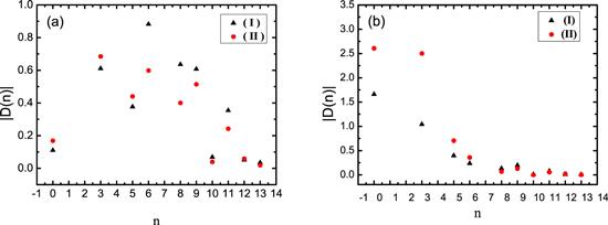
The second criterion is convergence of the operator product expansion. The absolute contributions of the vacuum condensates ∣D(n)∣ for the central values dependent on the energy scale parameter $\mu =\sqrt{{M}_{P}^{2}-{{\mathbb{M}}}_{c}^{2}}$ are shown in figure 1. D(n) is defined as(19)$\begin{eqnarray}D(n)=\displaystyle \frac{{\int }_{{m}_{c}^{2}}^{{s}_{0}}{\rm{d}}s\,{\rho }_{n}(s)\exp \left(-\tfrac{s}{{T}^{2}}\right)}{{\int }_{{m}_{c}^{2}}^{{s}_{0}}{\rm{d}}s\,\rho (s)\exp \left(-\tfrac{s}{{T}^{2}}\right)},\end{eqnarray}$where ρ_n(s) is the n dimension QCD spectral density, and $\rho (s)=\sqrt{s}{\rho }_{\mathrm{QCD}}^{1}(s)\pm {\rho }_{\mathrm{QCD}}^{0}(s)$ is the total spectral density. In this work, we carry out the operator product expansion up to the vacuum condensates of dimension 13 and assume vacuum saturation for the higher dimension vacuum condensates. We take the truncations n≤13 and k≤1 in a consistent way and discard the operators of the orders ${ \mathcal O }({\alpha }_{s}^{k})$ with k>1 [22]. From figure 1, we can see that the largest contribution comes from the vacuum condensates of dimension 6 for the scalar-diquark-scalar-diquark-antiquark type pentaquark state denoted as ${susc}{\overline{u}}_{1}$ with negative parity. The contributions from dimensions 10, 11, 12 and 13 are tiny. Therefore, the operator product expansion is convergent in this case. The axialvector-diquark-axialvector-diquark-antiquark type pentaquark state denoted as ${susc}{\overline{u}}_{2}$ with negative parity has the analogous situation. For the positive parity pentaquark states, the dominant contributions come from the perturbative terms, the operator product expansion is obviously convergent. For another two kinds of energy scale parameters, the convergence of the operator product expansion is also satisfied.

Figure 1.

New window|Download| PPT slide
Figure 1.The absolute contributions of the vacuum condensates of dimension n for central values dependent on the energy scale $\mu =\sqrt{{M}_{P}^{2}-{{\mathbb{M}}}_{c}^{2}}$, where (I) and (II) denote ${susc}{\bar{u}}_{1}$ and ${susc}{\bar{u}}_{2}$, respectively, (a) and (b) correspond to ${J}^{P}={\tfrac{1}{2}}^{-}$ and ${\tfrac{1}{2}}^{+}$, respectively.


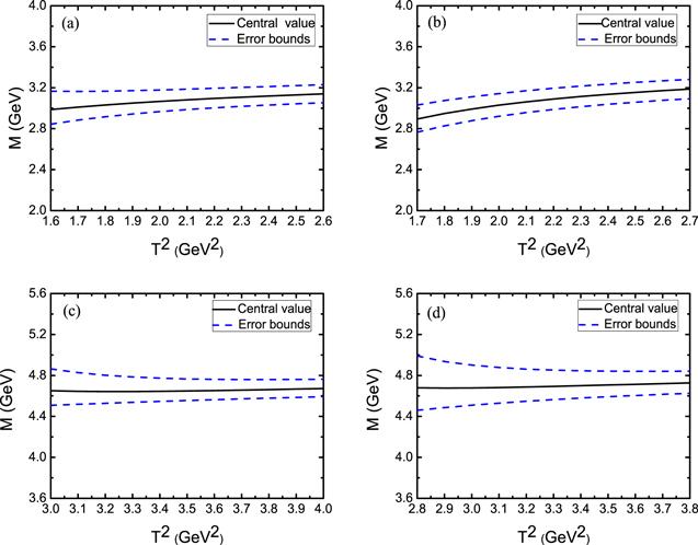
The third criterion is Borel platforms figures 2–7 show the masses and pole residues distribution with the variations of the Borel parameter T² at much larger intervals than the Borel windows as shown in table 1. It can be clearly seen that the uncertainties of the masses and pole residues from the Borel parameter T² in the Borel windows are very small, therefore, the Borel platforms exist. Now the three criteria are all satisfied.

Figure 2.

New window|Download| PPT slide
Figure 2.The masses of the charmed pentaquark states with variations of the Borel parameter T² dependent on the energy scale $\mu =\sqrt{{M}_{P}^{2}-{{\mathbb{M}}}_{c}^{2}}$, where (a)–(d) correspond to $\left({susc}{\bar{u}}_{1},{\tfrac{1}{2}}^{-}\right)$, $\left({susc}{\bar{u}}_{2},{\tfrac{1}{2}}^{-}\right)$, $\left({susc}{\bar{u}}_{1},{\tfrac{1}{2}}^{+}\right)$, and $\left({susc}{\bar{u}}_{2},{\tfrac{1}{2}}^{+}\right)$, respectively.

Figure 3.

New window|Download| PPT slide
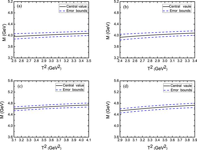
Figure 3.The masses of the charmed pentaquark states with variations of the Borel parameter T² dependent on the enery scale μ=1 GeV, where (a)–(d) correspond to $\left({susc}{\bar{u}}_{1},{\tfrac{1}{2}}^{-}\right)$, $\left({susc}{\bar{u}}_{2},{\tfrac{1}{2}}^{-}\right)$, $\left({susc}{\bar{u}}_{1},{\tfrac{1}{2}}^{+}\right)$, and $\left({susc}{\bar{u}}_{2},{\tfrac{1}{2}}^{+}\right)$, respectively.

Figure 4.

New window|Download| PPT slide
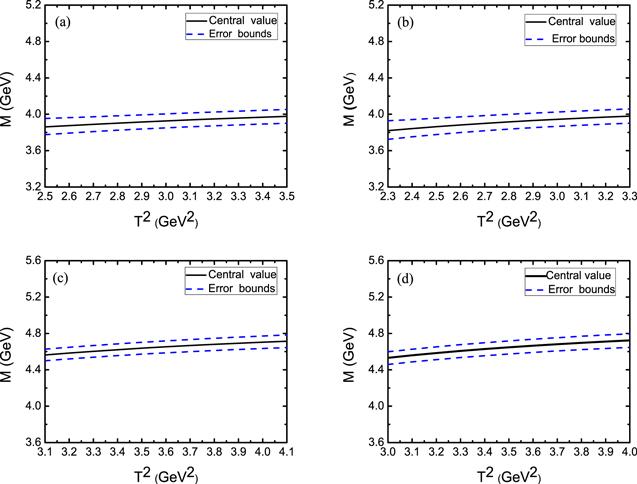
Figure 4.The masses of the charmed pentaquark states with variations of the Borel parameter T² dependent on the enery scale $\mu =\overline{1.0}\,\mathrm{GeV}$, where (a)–(d) correspond to $\left({susc}{\bar{u}}_{1},{\tfrac{1}{2}}^{-}\right)$, $\left({susc}{\bar{u}}_{2},{\tfrac{1}{2}}^{-}\right)$, $\left({susc}{\bar{u}}_{1},{\tfrac{1}{2}}^{+}\right)$, and $\left({susc}{\bar{u}}_{2},{\tfrac{1}{2}}^{+}\right)$, respectively.

Figure 5.

New window|Download| PPT slide
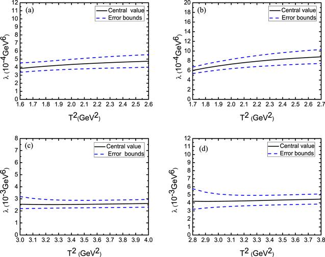
Figure 5.The pole residues of the charmed pentaquark states with variations of the Borel parameter T² dependent on the energy scale $\mu =\sqrt{{M}_{P}^{2}-{{\mathbb{M}}}_{c}^{2}}$, where (a)–(d) correspond to $\left({susc}{\bar{u}}_{1},{\tfrac{1}{2}}^{-}\right)$, $\left({susc}{\bar{u}}_{2},{\tfrac{1}{2}}^{-}\right)$, $\left({susc}{\bar{u}}_{1},{\tfrac{1}{2}}^{+}\right)$, and $\left({susc}{\bar{u}}_{2},{\tfrac{1}{2}}^{+}\right)$, respectively.

Figure 6.

New window|Download| PPT slide
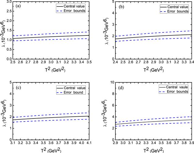
Figure 6.The pole residues of the charmed pentaquark states with variations of the Borel parameter T² dependent on the enery scale μ=1 GeV, where (a)–(d) correspond to $\left({susc}{\bar{u}}_{1},{\tfrac{1}{2}}^{-}\right)$, $\left({susc}{\bar{u}}_{2},{\tfrac{1}{2}}^{-}\right)$, $\left({susc}{\bar{u}}_{1},{\tfrac{1}{2}}^{+}\right)$, and $\left({susc}{\bar{u}}_{2},{\tfrac{1}{2}}^{+}\right)$, respectively.

Figure 7.

New window|Download| PPT slide
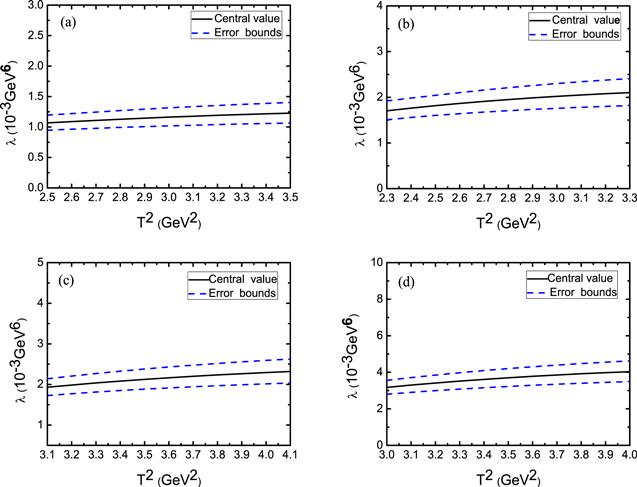
Figure 7.The pole residues of the charmed pentaquark states with variations of the Borel parameter T² dependent on the enery scale $\mu =\overline{1.0}\,\mathrm{GeV}$, where (a)–(d) correspond to $\left({susc}{\bar{u}}_{1},{\tfrac{1}{2}}^{-}\right)$, $\left({susc}{\bar{u}}_{2},{\tfrac{1}{2}}^{-}\right)$, $\left({susc}{\bar{u}}_{1},{\tfrac{1}{2}}^{+}\right)$, and $\left({susc}{\bar{u}}_{2},{\tfrac{1}{2}}^{+}\right)$, respectively.


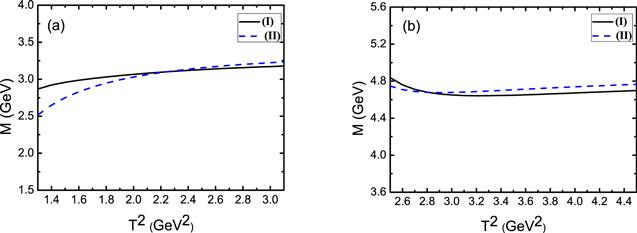
Figure 8 shows the masses distribution with the Borel parameter for central values on a large scale dependent on the energy scale $\mu =\sqrt{{M}_{P}^{2}-{{\mathbb{M}}}_{c}^{2}}$. It is seen that the predicted masses increase slowly with the Borel parameter for the negative parity. For the positive parity the predicted masses decrease slowly with the Borel parameter. It warrants the appearance of good Borel platforms.

Figure 8.

New window|Download| PPT slide
Figure 8.The predicted masses with variations of the Borel parameter for central values dependent on the energy scale $\mu =\sqrt{{M}_{P}^{2}-{{\mathbb{M}}}_{c}^{2}}$, where (I) and (II) denote the pentaquark states ${susc}{\bar{u}}_{1}$ and ${susc}{\bar{u}}_{2}$, respectively, (a) and (b) correspond to ${J}^{P}={\tfrac{1}{2}}^{-}$ and ${\tfrac{1}{2}}^{+}$, respectively.


Considering all uncertainties of the parameters, we obtain the masses and pole residues of the charmed pentaquark states with ${J}^{P}={\tfrac{1}{2}}^{\pm }$ based on three types of energy scale parameters as shown in table 2. It is seen that the predicted masses of the charmed pentaquark states ${susc}{\bar{u}}_{1}$ and ${susc}{\bar{u}}_{2}$ with ${J}^{P}={\tfrac{1}{2}}^{-}$ dependent on the energy scale parameter $\mu =\sqrt{{M}_{P}^{2}-{{\mathbb{M}}}_{c}^{2}}$ are ${3.08}_{-0.14}^{+0.12}\,\mathrm{GeV}$ and ${3.09}_{-0.17}^{+0.14}\,\mathrm{GeV}$ respectively, which are in consistent with the experiment data of the LHCb collaboration [1]. The masses of the charmed pentaquark states ${susc}{\bar{u}}_{1}$ and ${susc}{\bar{u}}_{2}$ with ${J}^{P}={\tfrac{1}{2}}^{+}$ dependent on the energy scale parameter $\mu =\sqrt{{M}_{P}^{2}-{{\mathbb{M}}}_{c}^{2}}$ are ${4.65}_{-0.11}^{+0.11}\,\mathrm{GeV}$ and ${4.69}_{-0.16}^{+0.15}\,\mathrm{GeV}$ respectively, which have large deviation to the five new excited states. The predicated masses based on the other two kinds of energy scale parameters are larger than that based on the energy scale formula $\mu =\sqrt{{M}_{P}^{2}-{{\mathbb{M}}}_{c}^{2}}$.


Table 2.
Table 2.The predicted masses and pole residues of the charmed pentaquark states.

	JP	μ(GeV)	M (GeV)	λ (GeV6)
${susc}{\bar{u}}_{1}$	${\tfrac{1}{2}}^{-}$	2.5	${3.08}_{-0.14}^{+0.12}$	${4.42}_{-0.75}^{+0.89}\times {10}^{-4}$
		1.0	${4.02}_{-0.10}^{+0.10}$	${1.17}_{-0.17}^{+0.20}\times {10}^{-3}$
		$\overline{1.0}$	${3.93}_{-0.10}^{+0.09}$	${1.16}_{-0.17}^{+0.19}\times {10}^{-3}$
${susc}{\bar{u}}_{2}$	${\tfrac{1}{2}}^{-}$	2.6	${3.09}_{-0.17}^{+0.14}$	${7.88}_{-1.52}^{+1.78}\times {10}^{-4}$
		1.0	${4.02}_{-0.11}^{+0.11}$	${1.99}_{-0.32}^{+0.36}\times {10}^{-3}$
		$\overline{1.0}$	${3.92}_{-0.12}^{+0.10}$	${1.95}_{-0.31}^{+0.35}\times {10}^{-3}$
${susc}{\bar{u}}_{1}$	${\tfrac{1}{2}}^{+}$	4.3	${4.65}_{-0.11}^{+0.11}$	${2.54}_{-0.31}^{+0.35}\times {10}^{-3}$
		1.0	${4.68}_{-0.09}^{+0.10}$	${1.94}_{-0.30}^{+0.33}\times {10}^{-3}$
		$\overline{1.0}$	${4.65}_{-0.09}^{+0.10}$	${2.17}_{-0.32}^{+0.35}\times {10}^{-3}$
${susc}{\bar{u}}_{2}$	${\tfrac{1}{2}}^{+}$	4.3	${4.69}_{-0.16}^{+0.15}$	${4.28}_{-0.72}^{+0.70}\times {10}^{-3}$
		1.0	${4.65}_{-0.12}^{+0.11}$	${3.19}_{-0.57}^{+0.64}\times {10}^{-3}$
		$\overline{1.0}$	${4.65}_{-0.12}^{+0.10}$	${3.70}_{-0.62}^{+0.69}\times {10}^{-3}$

New window|CSV

The predicted uncertainties originate from the input parameters, such as the effective c-quark mass ${{\mathbb{M}}}_{c}$, the continuum threshold parameter s₀, and the vacuum condensate values ${m}_{0}^{2}$, $\langle \bar{s}s\rangle $ and $\langle \bar{q}q\rangle $, in which the parameters s₀ and ${m}_{0}^{2}$ cause main uncertainties. For example, for the charmed pentaquark states ${susc}{\bar{u}}_{1}$ with ${J}^{P}={\tfrac{1}{2}}^{-}$, the uncertainties from s₀ and ${m}_{0}^{2}$ are ${}_{-0.08}^{+0.09}\mathrm{GeV}$ and ${}_{-0.11}^{+0.09}\mathrm{GeV}$, respectively.

From table 2, we can see that the masses of the negative-parity pentaquark states from two different interpolating currents lie in the same region. Generally speaking, an interpolating current can couple to a hadron or several hadrons or a hadron system or several hadron systems if they have the same quantum numbers, as the non-vanishing couplings are not forbidden by the symmetries. On the other hand, a hadron maybe have many Fock states, a Fock state couples potentially to an interpolating current with the same quantum numbers as the Fock state. Therefore, the present calculations could indicate that a pentaquark state owns two different inner structures, or two pentaquark states have masses in the same region. More experimental and theoretical works are still needed to make a solid assignment. In addition, it is found that the mass gaps between the positive-parity pentaquark states and the corresponding negative-parity pentaquark states are more than 1.5 GeV. If the positive-parity pentaquark states are the orbitally excited states of the negative-parity ones, the mass splittings seem too large because the energy costs exciting an orbital angular momentum are approximately 300–600 MeV. However, our calculation results are obtained based on the quantum chromodynamics, which are different from the ones based on the quark model, the positive-parity pentaquark states are not necessarily the orbitally excited states of the negative-parity ones. The currents J₁(x) and J₂(x) have negative-parity, they also couple potentially to the positive-parity pentaquark states, as multiplying iγ₅ to the currents to change their parity [40–43].

For the positive-parity pentaquark states, the contribution of the vacuum condensate of dimension n in the QCD spectral density ${\rho }_{{\rm{QCD}}}^{1}(s)$ with n≥3 is canceled out with the corresponding ones in the QCD spectral density ${\rho }_{{\rm{QCD}}}^{0}(s)$ to a great extent due to the combination $\sqrt{s}{\rho }_{{\rm{QCD}}}^{1}(s)-{\rho }_{{\rm{QCD}}}^{0}(s)$, the operator product expansion converges very well at all the energy scales μ≥1 GeV. In such a case, the energy scale formula $\mu =\sqrt{{M}_{P}^{2}-{{\mathbb{M}}}_{c}^{2}}$ can only improve the pole contributions mildly and enhance the operator product expansion convergence mildly, therefore the predicted pentaquark masses depend on the energy scales of the QCD spectral densities mildly. For the negative-parity pentaquark states, the contribution of the vacuum condensate of dimension n in the QCD spectral density ${\rho }_{{\rm{QCD}}}^{1}(s)$ with n≥3 is strengthened by the corresponding ones in the QCD spectral density ${\rho }_{{\rm{QCD}}}^{0}(s)$ due to the combination $\sqrt{s}{\rho }_{{\rm{QCD}}}^{1}(s)+{\rho }_{{\rm{QCD}}}^{0}(s)$, the operator product expansion converges very slow. In this case, the energy scale formula $\mu =\sqrt{{M}_{P}^{2}-{{\mathbb{M}}}_{c}^{2}}$ can improve the pole contributions remarkably and enhance the operator product expansion convergence remarkably, we prefer the energy scale formula $\mu =\sqrt{{M}_{P}^{2}-{{\mathbb{M}}}_{c}^{2}}$ to choose the best energy scales of the QCD spectral densities to obtain the ideal Borel windows to extract the pentaquark masses, as the predictions vary considerably with variations of the Borel windows.

4. Conclusion

In this work, we construct both the scalar-diquark-scalar-diquark-antiquark type and axialvector-diquark-axialvector-diquark-antiquark type interpolating currents to study the charmed pentaquark states ${susc}\bar{u}$ with ${J}^{P}={\tfrac{1}{2}}^{\pm }$. We employ three types of energy scale parameters to investigate the masses and pole residues of the charmed pentaquark states using the QCD sum rules. By comparing these results with experiment data, we find that if we take pole contributions in the scope of 40%–60% we can get more reasonable prediction using the energy scale formula $\mu =\sqrt{{M}_{P}^{2}-{{\mathbb{M}}}_{c}^{2}}$ than the other two types of energy scale parameters. The energy scale formula $\mu =\sqrt{{M}_{P}^{2}-{{\mathbb{M}}}_{c}^{2}}$ can improve the pole contributions dramatically and enhance the operator product expansion convergence remarkably, especially for the negative parity states. Hence, we prefer the energy scale formula $\mu =\sqrt{{M}_{P}^{2}-{{\mathbb{M}}}_{c}^{2}}$ in this work. Our calculation results support assigning the new excited Ω_c states to be the scalar-diquark-scalar-diquark-antiquark type and axialvector-diquark-axialvector-diquark-antiquark type charmed pentaquark states ${susc}\bar{u}$ with ${J}^{P}={\tfrac{1}{2}}^{-}$. It indicates that the pentaquark configuration can be possible interpretation of the new narrow excited states observed in the LHCb collaboration.

We group the flavor parts as $({su})-({sc})-\bar{u}$ to construct the interpolating currents here. If we group the flavor parts as $({ss})-({cu})-\bar{u}$ to construct the scalar-diquark-scalar-diquark-antiquark type interpolating current, which is non-existent according to fermi statistics. We can construct axialvector-diquark-axialvector-diquark-antiquark type interpolating current by grouping the flavor parts as $({ss})-({cu})-\bar{u}$. The result should approximately equal to that by grouping the flavor parts as $({su})-({sc})-\bar{u}$ according to the SU(3) symmetry. Further calculation is still needed to make a solid conlcusion.

Acknowledgments

This work is supported by National Natural Science Foundation, Grant Number 11775079.

Reference View Option By original order
By published year
By cited within times
By Impact factor

[1]Aaij R et al. 2017 Phys. Rev. Lett. 118182001
DOI:10.1103/PhysRevLett.118.182001 [Cited within: 2]

[2]Wang W Zhu R L 2017 Phys. Rev. D 96014024
DOI:10.1103/PhysRevD.96.014024 [Cited within: 1]

[3]Cheng H Y Chiang C W 2017 Phys. Rev. D 95094018
DOI:10.1103/PhysRevD.95.094018

[4]Chen H X Mao Q Chen W Hosaka A Liu X Zhu S L 2017 Phys. Rev. D 95094008
DOI:10.1103/PhysRevD.95.094008

[5]Chen B Liu X 2017 Phys. Rev. D 96094015
DOI:10.1103/PhysRevD.96.094015

[6]Karliner M Rosner J L 2017 Phys. Rev. D 95114012
DOI:10.1103/PhysRevD.95.114012

[7]Wang K L Xiao L Y Zhong X H Zhao Q 2017 Phys. Rev. D 95116010
DOI:10.1103/PhysRevD.95.116010

[8]Padmanath M Mathur N 2017 Phys. Rev. Lett. 119042001
DOI:10.1103/PhysRevLett.119.042001

[9]Agaev S S Azizi K Sundu H 2017 Eur. Phys. J. C 77 395
DOI:10.1140/epjc/s10052-017-4953-z [Cited within: 1]

[10]Agaev S S Azizi K Sundu H 2017 Europhys. Lett. 118 61001
DOI:10.1209/0295-5075/118/61001 [Cited within: 1]

[11]Zhao Z Ye D D Zhang A 2017 Phys. Rev. D 95114024
DOI:10.1103/PhysRevD.95.114024 [Cited within: 2]

[12]Wang Z G Wei X N Yan Z H 2017 Eur. Phys. J. C 77 832
DOI:10.1140/epjc/s10052-017-5409-1 [Cited within: 2]

[13]Wang Z G 2017 Eur. Phys. J. C 77 325
DOI:10.1140/epjc/s10052-017-4895-5 [Cited within: 3]

[14]Aajj R et al. 2015 Phys. Rev. Lett. 115072001
DOI:10.1103/PhysRevLett.115.072001 [Cited within: 1]

[15]Yuan S G An C S Wei K W Zou B S Xu H S 2013 Phys. Rev. C 87025205
DOI:10.1103/PhysRevC.87.025205 [Cited within: 1]

[16]Kim H C Polyakov M V Praszalowicz M Yang G S 2017 Phys. Rev. D 96094021
DOI:10.1103/PhysRevD.96.094021 [Cited within: 1]

[17]An C S Chen H 2017 Phys. Rev. D 96034012
DOI:10.1103/PhysRevD.96.034012 [Cited within: 1]

[18]Yang G Ping J 2018 Phys. Rev. D 97034023
DOI:10.1103/PhysRevD.97.034023 [Cited within: 1]

[19]Huang Y Xiao C J Lu Q F Wang R He J Geng L S 2018 Phys. Rev. D 97094013
DOI:10.1103/PhysRevD.97.094013 [Cited within: 1]

[20]Wang C Liu L L Kang X W Guo X H 2018 Eur. Phys. J. C 78 407
DOI:10.1140/epjc/s10052-018-5874-1

[21]Huang H Ping J Wang F 2018 Phys. Rev. D 97034027
DOI:10.1103/PhysRevD.97.034027 [Cited within: 1]

[22]Wang Z G Zhang J X 2018 Eur. Phys. J. C 78 503
DOI:10.1140/epjc/s10052-018-5989-4 [Cited within: 3]

[23]Reinders L J Rubinstein H Yazaki S 1985 Phys. Rep. 127 1
DOI:10.1016/0370-1573(85)90065-1 [Cited within: 4]

[24]Wang Z G Huang T 2016 Eur. Phys. J. C 76 43
DOI:10.1140/epjc/s10052-016-3880-8 [Cited within: 4]

Wang Z G 2016 Eur. Phys. J. C 76 142
DOI:10.1140/epjc/s10052-016-3880-8 [Cited within: 4]

[25]Wang Z G Zhang J X 2018 Eur. Phys. J. C 78 14
DOI:10.1140/epjc/s10052-017-5514-1 [Cited within: 1]

[26]Wang Z G Huang T 2014 Nucl. Phys. A 930 63
DOI:10.1016/j.nuclphysa.2014.08.084

[27]Wang Z G 2014 Eur. Phys. J. C 74 2874
DOI:10.1140/epjc/s10052-014-2874-7 [Cited within: 3]

[28]Wang Z G 2020 Int. J. Mod. Phys. A 352050003
DOI:10.1142/S0217751X20500037 [Cited within: 1]

[29]Wang Z G 2020 Chin. Phys. C 44063105
DOI:10.1088/1674-1137/44/6/063105 [Cited within: 1]

[30]Patrignani C et al. 2016 Chin. Phys. C 40100001
DOI:10.1088/1674-1137/40/10/100001 [Cited within: 2]

[31]Narison S Tarrach R 1983 Phys. Lett. B 125 217
DOI:10.1016/0370-2693(83)91271-6

[32]Narison S 2002 QCD as a Theory of Hadrons: From Partons to Confinement 17CambridgeCambridge University Press
DOI:10.1017/CBO9780511535000 [Cited within: 1]

[33]Wang Z G 2016 Eur. Phys. J. C 76 387
DOI:10.1140/epjc/s10052-016-4238-y [Cited within: 1]

[34]Wang Z G 2010 Eur. Phys. J. C 70 139
DOI:10.1140/epjc/s10052-010-1447-7 [Cited within: 1]

[35]Wang Z G Liu Z C Zhang X H 2009 Eur. Phys. J. C 64 373
DOI:10.1140/epjc/s10052-009-1156-2 [Cited within: 1]

[36]Matheus R D Narison S Nielsen M Richard J M 2007 Phys. Rev. D 75014005
DOI:10.1103/PhysRevD.75.014005 [Cited within: 1]

[37]Navarra F S Nielsen M 2006 Phys. Lett. B 639 272
DOI:10.1016/j.physletb.2006.06.054 [Cited within: 1]

[38]Wang Z G 2011 Eur. Phys. J. A 47 81
DOI:10.1140/epja/i2011-11081-8 [Cited within: 1]

[39]Wang Z G 2012 Commun. Theor. Phys. 58 723
DOI:10.1088/0253-6102/58/5/17

[40]Wang Z G 2010 Eur. Phys. J. C 68 479
DOI:10.1140/epjc/s10052-010-1365-8 [Cited within: 2]

[41]Chung Y Dosch H G Kremer M Schall D 1982 Nucl. Phys. B 197 55
DOI:10.1016/0550-3213(82)90154-7

[42]Bagan E Chabab M Dosch H G Narison S 1993 Phys. Lett. B 301 243
DOI:10.1016/0370-2693(93)90696-F

[43]Jido D Kodama N Oka M 1996 Phys. Rev. D 54 4532
DOI:10.1103/PhysRevD.54.4532 [Cited within: 1]