Salman Ahmad^,1,*, T. Hayat^1,2, A. Alsaedi², Z. H. Khan^3,4, M. Waleed Ahmed Khan¹1 Department of Mathematics, Quaid-I-Azam University 45320,Islamabad 44000, Pakistan
2 Nonlinear Analysis and Applied Mathematics (NAAM) Research Group, Department of Mathematics, Faculty of Science, King Abdulaziz University,P.O. Box 80257, Jeddah 21589, Saudi Arabia
3 State Key Laboratory of Hydraulics and Mountain River Engineering, College of Water Resource and Hydropower, Sichuan University, Chengdu 610065, China
4 Key Laboratory of Advanced Reactor Engineering and Safety, Ministry of Education, Tsinghua University, Beijing 100084, China

Corresponding authors: * E-mail:asalman@math.qau.edu.pk

Received:2019-05-21Online:2019-11-1


Abstract
This article computes effect of uniform magnetic field on nanofluid flow filling porous medium inside parallel sheets. Darcy's law is used to characterize porous medium. Flow is caused by stretching of the lower sheet. The governing systems are computed using Finite difference technique. This scheme is used due to its more general and powerful nature to solve nonlinear problems. Results are obtained and discussed graphically. Nusselt number, skin friction, streamlines, velocity and temperature are emphasized.
Keywords： finite difference scheme;porous medium;magnetic field;nanofluid;parallel stretchable sheets


PDF (1803KB)MetadataMetricsRelated articlesExportEndNote|Ris|BibtexFavorite
Cite this article
Salman Ahmad, T. Hayat, A. Alsaedi, Z. H. Khan, M. Waleed Ahmed Khan. Finite Difference Analysis of Time-Dependent Viscous Nanofluid Flow Between Parallel Plates. [J], 2019, 71(11): 1293-1300 doi:10.1088/0253-6102/71/11/1293

1 Introduction

Heat transfer rate has played a key role in saving energy and experimental costs. Presently technological fields need devices with more precision, accurate functioning, higher performance and more lifespan. That is why researchers are working for the thermal properties of materials. Nanofluids are the mixture of nanosized metallic as well as nonmetallic particles in some base fluids used for increasing thermal conductivity of fluids. In $1995$ Choi^[1] found the enhanced thermal properties of nanofluids as compared to simple fluids which compelled other researchers to give attention to such nanosized particles with extraordinary characteristics. Moreover, Buongiorno^[2] discussed seven slip phenomena of nanofluid (i.e. inertia, Brownian diffusion, fluid drainage, diffusiophoresis, gravity, thermophoresis and Magnus). However he concluded that Brownian motion and thermophoresis are the key slip phenomena. Different types of particles e.g. copper (Cu), gold (Au), silver (Ag), and nickel (Ni), metal oxides like copper oxide (CuO), silicon dioxide (SiO$_2$), oxide (Fe$_2$O$_3)$, iron (III), titanium dioxide (TiO$_2)$ etc.^[3-8] are extensively used by different researchers. Flow of nanofluid due to a rotating disk is examined by Turkyilmazoglu.^[9] For cooling process, spraying of nanofluid by a rotating inclined disk is numerically investigated by Sheikholeslami et al.^[10]



Nomenclature

New window|CSV

Magnetohydrodynamic flows over a stretching sheet have diverse applications in industrial processes. Examples of such processes include polymer sheet industries, cooling processes in many industries, glass sheets, parmachaology, biotechnology, nuclear research, glass sheet industries, drawing of plastic sheets, polymers extrusion, cooling processes of melting materials etc. In all such cases the flow situation is of vital importance. Quality of end product mainly depends upon the rate of heat transfer and skin friction. Such processes also depend on the boundary layer phenomenon along stretching surfaces as well as the mass transfer rate. Rajogopal et al.^[11] initially studied viscoelastic fluid flow phenomenon caused by a stretching surface. MHD flow by a vertical plate was examined by Riley.^[12] Fairbanks and Wike^[13] analyzed the effect of chemical reaction in a uniform fluid flow over a horizontal sheet. Andersson et al.^[14] investigated chemically reactive flow over a stretching surface. The impacts of magnetic dipole and thermal radiation on Willamsion fluid flow are discussed by Hayat et al.^[15] Some more applications are highlighted by Magyari and Keller.^[16-17]

Formulation of flow problems in the form of partial or ordinary differential equations is very important for precise modeling and simulation in engineering processes. These classes of differential equations are tackled both analytically as well as numerically. In this article numerical approach has been utilized to tackle the partial differential equations governing the problem of MHD flow of nanofluid in porous medium between two stretchable sheets. Applications of finite difference scheme^[18-20] have been studied for solving the system of partial differential equations. Graphical results are obtained through various involved parameters for velocity, concentration and temperature. Quantities of engineering interests i.e. skin friction, mass and heat transfer rates are also discussed through graph. Main points of the present article are summarized in the concluding section.

2 Mathematical Modeling

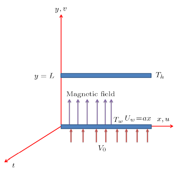
In this section we model the flow of time-dependent viscous nanofluid inside two parallel sheets. Nanofluid occupies porous medium and Darcy's law is used to characterized porous space. Influence of magnetic field is perpendicular to x-axis. Injection is taken on porous lower plate with stretching rate $a$. Upper plate is at a distance $L$ from lower plate. Temperature of lower plate is $T_w$ and upper plate $T_h$. Figure 1 shows the flow diagram. Under the considered assumptions the flow expressions are:

(1) $$ \frac{\partial u}{\partial x}+\frac{\partial v}{\partial y}=0\,, $$
(2) $$ \Big(\frac{\partial }{\partial t}+u\frac{\partial }{\partial x}+v\frac{\partial }{\partial y}\Big)u \\ \quad =\nu\Big(\frac{\partial^2}{\partial x^2}+\frac{\partial^2}{\partial y^2}\Big)u-\Big(\frac{\sigma B_0^2}{\rho}+\frac{\nu}{k^*}\Big)u\,, $$
(3) $$ \Big(\frac{\partial }{\partial t}+u\frac{\partial }{\partial x}+v\frac{\partial }{\partial y}\Big)v =\nu\Big(\frac{\partial^2}{\partial x^2}+\frac{\partial^2}{\partial y^2}\Big)v-\frac{\nu}{k^*}v\,, $$
(4) $$ \Big(\frac{\partial }{\partial t}+u\frac{\partial }{\partial x}+v\frac{\partial }{\partial y}\Big)T \\ \quad =\frac{k}{\rho c_p}\Big(\frac{\partial^2}{\partial x^2}+\frac{\partial^2}{\partial y^2}\Big)T+\tau^*\Big[D_B\Big(\frac{\partial T}{\partial x}\frac{\partial C}{\partial x} +\frac{\partial C}{\partial y}\frac{\partial C}{\partial y}\Big) \\ \qquad +\frac{D_T}{T_h}\Big\{\Big(\frac{\partial T}{\partial x}\Big)^2+\Big(\frac{\partial T}{\partial y}\Big)^2\Big\}\Big]\,, $$
(5) $$ \Big(\frac{\partial }{\partial t}+u\frac{\partial }{\partial x}+v\frac{\partial }{\partial y}\Big)C \\ \quad =D_B\Big(\frac{\partial^2 }{\partial x^2}+\frac{\partial^2 }{\partial y^2}\Big)C+\frac{D_T}{T_h}\Big(\frac{\partial^2}{\partial x^2}+\frac{\partial^2}{\partial y^2}\Big)T\,, $$

Fig. 1

New window|Download| PPT slide
Fig. 1(Color online) Flow diagram.



with constraints

(6) $$ u(0,x,y)=0\,, \quad v(0,x,y)=0\,, \quad T(0,x,y)=T_w\,, \\ C(0,x,y)=C_w\,,\quad u(t,x,0)=ax\,, \quad v(t,x,0)=V_0\,, \\ T(t,x,0)=T_w\,, \quad C(t,x,0)=C_w\,,\quad u(t,x,L)=0\,, \\ v(t,x,L)=0\,, \quad T(t,x,L)=T_h\,, \quad C(t,x,L)=C_h\,. $$
In order to transform the system into dimensionless form, consider the dimensionless variables

(7) $$ \tau=\frac{\nu}{L^2}t\,,\quad \eta=\frac{y}{L}\,,\quad \xi=\frac{x}{L}\,,\quad U(\tau,\xi,\eta)=\frac{L}{\nu}u\,, \\ Sc=\frac{\nu}{D_B}\,,\quad V(\tau,\xi,\eta)=\frac{L}{\nu}v\,,\quad \phi(\tau,\xi,\eta)=\frac{C-C_h}{C_w-C_h}\,, \\ \theta(\tau,\xi,\eta)=\frac{T-T_h}{T_w-T_h}\,,\quad Ha=\frac{\sigma B_0^2}{a\rho}\,, \\ Pr=\frac{\mu c_p}{k}\,,\quad \lambda=\frac{\nu}{ak^*}\,, \quad Nt=\tau^*\frac{(T_w-T_h)D_T}{T_h\nu}\,, \\ Nb=\tau^*\frac{(C_w-C_h)D_B}{\nu}\,, \quad \beta=\frac{LV_0}{\nu}\,,\quad M=\frac{aL^2}{\nu}\,. $$
Using dimensionless variables the flow expressions are reduced to

(8) $$ \frac{\partial U}{\partial \xi}+\frac{\partial V}{\partial \eta}=0\,, $$
(9) $$ \frac{\partial U}{\partial \tau}+U\frac{\partial U}{\partial \xi}+V\frac{\partial U}{\partial \eta}=\frac{\partial^2U}{\partial \xi^2}+\frac{\partial^2U}{\partial \eta^2}-\frac{Ha+\lambda}{1/M}U\,, $$
(10) $$ \frac{\partial V}{\partial \tau}+U\frac{\partial V}{\partial \xi}+V\frac{\partial V}{\partial \eta}=\frac{\partial^2V}{\partial \xi^2}+\frac{\partial^2V}{\partial \eta^2}-\frac{\lambda}{1/M} V\,, $$
(11) $$ \frac{\partial \theta}{\partial \tau}+U\frac{\partial \theta}{\partial \xi}+V\frac{\partial \theta}{\partial \eta}=\frac{1}{Pr}\Big(\frac{\partial^2\theta}{\partial \xi^2} +\frac{\partial^2\theta}{\partial \eta^2}\Big) \quad\;\; +Nb\Big(\frac{\partial \theta}{\partial \xi}\frac{\partial\phi}{\partial\xi}+\frac{\partial\theta}{\partial\eta} \frac{\partial\phi}{\partial\eta}\Big) +Nt\Big\{\Big(\frac{\partial\theta}{\partial\xi}\Big)^2 +\Big(\frac{\partial\theta}{\partial\eta}\Big)^2\Big\}\,, $$
(12) $$ \frac{\partial \phi}{\partial \tau}+U\frac{\partial \phi}{\partial \xi}+V\frac{\partial \phi}{\partial \eta}=\frac{1}{Sc}\Big[\frac{\partial^2\phi}{\partial \xi^2}+\frac{\partial^2\phi}{\partial \eta^2}\Big] \quad\quad +\frac{Nt}{Nb Sc}\Big[\frac{\partial^2\theta}{\partial \xi^2}+\frac{\partial^2\theta}{\partial \eta^2}\Big]\,, $$
(13) $$ U(0,\xi,\eta)=0\,,\quad V(0,\xi,\eta)=0\,, \quad \theta(0,\xi,\eta)=1\,, \\ \phi(0,\xi,\eta)=1\,,\quad U(\tau,\xi,0)=M\xi\,,\quad V(\tau,\xi,0)=\beta\,, \\ \theta(\tau,\xi,0)=1\,,\quad \phi(\tau,\xi,0)=1\,,\quad U(\tau,\xi,L)=0\,, \\ V(\tau,\xi,L)=0\,, \quad \theta(\tau,\xi,L)=0\,,\quad \phi(\tau,\xi,L)=0\,. $$

3 Quantities of Engineering Interest

Sherwood number, Nusselt number and skin friction are defined as

(14) $$ Sh_x=\frac{x q_m}{D_B(C_w-C_h)}\,,\quad Nu_{x}=\frac{xq_w}{k(T_w-T_h)}\,,\quad C_{f_x}=\frac{-2\tau_w}{\rho(ax)^2}\,, $$
where $q_m$ represents mass flux, $q_w$ heat flux and $\tau_w$ shear stress. These are

(15) $$ q_m=-D_B\Big(\frac{\partial C}{\partial x}+\frac{\partial C}{\partial y}\Big)\Big|_{y=0}\,,\quad q_w=-k\Big(\frac{\partial T}{\partial x}+\frac{\partial T}{\partial y}\Big)\Big|_{y=0}\,,\quad \tau=\mu\Big(\frac{\partial v}{\partial x}+\frac{\partial u}{\partial y}\Big)\Big|_{y=0}\,. $$
In dimensionless forms the Sherwood number, Nusselt number and skin friction are given by

(16) $$ Sh_x=-\xi\Big(\frac{\partial \phi}{\partial\xi}+\frac{\partial \phi}{\partial\eta}\Big)\Big|_{\eta=0}\,,\quad Nu_x=-\xi\Big(\frac{\partial\theta}{\partial\xi}+\frac{\partial\theta}{\partial\eta}\Big)\Big|_{\eta=0}\,, \quad C_{f_x}=\frac{-2}{M^2\xi^2}\Big(\frac{\partial V}{\partial\xi}+\frac{\partial U}{\partial\eta}\Big)\Big|_{\eta=0}\,. $$

4 Constructing Finite Difference Scheme

In order to solve the partial differential system given in Eqs. (8)--(12) with constraints $(13)$, we used Finite difference scheme. The system contains four unknown function $(U,V,\theta,\phi)$ and three independent variables $(\tau,\xi,\eta)$. On the basis of finite difference technique, FD toolkit for partial derivatives are given by

(17) $$ \frac{\partial U}{\partial \tau}=\frac{U_{i,j}^{n+1}-U_{i,j}^n}{\triangle\tau}\,,\quad \frac{\partial \phi}{\partial \tau}=\frac{\phi_{i,j}^{n+1}-\phi_{i,j}^n}{\triangle\tau}\,,\quad \frac{\partial \theta}{\partial \tau}=\frac{\theta_{i,j}^{n+1}-\theta_{i,j}^n}{\triangle\tau}\,,\quad \frac{\partial V}{\partial \tau}=\frac{V_{i,j}^{n+1}-V_{i,j}^n}{\triangle\tau}\,, \\ \frac{\partial V}{\partial \xi}=\frac{V_{i+1,j}^n-V_{i,j}^n}{\triangle\xi}\,,\quad \frac{\partial \phi}{\partial \xi}=\frac{\phi_{i+1,j}^n-\phi_{i,j}^n}{\triangle\xi}\,,\quad \frac{\partial \theta}{\partial \xi}=\frac{\theta_{i+1,j}^n-\theta_{i,j}^n}{\triangle\xi}\,,\quad \frac{\partial U}{\partial \eta}=\frac{U_{i,j+1}^n-U_{i,j}^n}{\triangle\eta}\,,\\ \frac{\partial \theta}{\partial \eta}=\frac{\theta_{i,j+1}^n-\theta_{i,j}^n}{\triangle\eta}\,,\quad \frac{\partial^2 \phi}{\partial \xi^2}=\frac{\phi_{i+1,j}^n-2\phi_{i,j}^n+\phi_{i-1,j}^n}{(\triangle\xi)^2}\,,\quad \frac{\partial^2 U}{\partial \xi^2}=\frac{U_{i+1,j}^n-2U_{i,j}^n+U_{i-1,j}^n}{(\triangle\xi)^2}\,, \\ \frac{\partial^2 \theta}{\partial \xi^2}=\frac{\theta_{i+1,j}^n-2\theta_{i,j}^n+\theta_{i-1,j}^n}{(\triangle\xi)^2}\,,\quad \frac{\partial U}{\partial \xi}=\frac{U_{i+1,j}^n-U_{i,j}^n}{\triangle\xi}\,,\quad \frac{\partial^2 U}{\partial \eta^2}=\frac{U_{i,j+1}^n+U_{i,j-1}^n-2U_{i,j}^n}{(\triangle\eta)^2}\,,\\ \frac{\partial^2 V}{\partial \eta^2}=\frac{V_{i,j+1}^n+V_{i,j-1}^n-2V_{i,j}^n}{(\triangle\eta)^2}\,,\quad \frac{\partial^2 \theta}{\partial \eta^2}=\frac{\theta_{i,j+1}^n-2\theta_{i,j}^n+\theta_{i,j-1}^n}{(\triangle\eta)^2}\,,\quad \frac{\partial V}{\partial \eta}=\frac{V_{i,j+1}^n-V_{i,j}^n}{\triangle\eta}\,,\\ \frac{\partial \phi}{\partial \eta}=\frac{\phi_{i,j+1}^n-\phi_{i,j}^n}{\triangle\eta}\,, \quad \frac{\partial^2 V}{\partial \xi^2}=\frac{V_{i+1,j}^n-2V_{i,j}^n+V_{i-1,j}^n}{(\triangle\xi)^2}\,, \quad \frac{\partial^2 \phi}{\partial \eta^2}=\frac{\phi_{i+1,j}^n-2\phi_{i,j}^n+\phi_{i-1,j}^n}{(\triangle\eta)^2}\,. $$
Using Eq. (17), partial differential equations system (Eqs. (7)--(10)) are reduced to

(18) $$ \frac{U_{i+1,j}^{n}-U_{i,j}^n}{\triangle\xi}+\frac{V_{i,j+1}^{n}-V_{i,j}^n}{\triangle\eta}=0\,, $$
(19) $$ \frac{U_{i,j}^{n+1}-U_{i,j}^n}{\triangle\tau}+U_{i,j}^{n} \frac{U_{i+1,j}^{n}-U_{i,j}^n}{\triangle\xi} +V_{i,j}^{n}\frac{U_{i,j+1}^{n}-U_{i,j}^n}{\triangle\eta} =\frac{U_{i+1,j}^n-2U_{i,j}^n+U_{i-1,j}^n}{(\triangle\xi)^2} \\ \quad + \frac{U_{i,j+1}^n-2U_{i,j}^n+U_{i,j-1}^n}{(\triangle\eta)^2}-\frac{Ha+\lambda}{1/M}U_{i,j}^n\,, $$
(20) $$ \frac{V_{i,j}^{n+1}-V_{i,j}^n}{\triangle\tau}+U_{i,j}^{n}\frac{V_{i+1,j}^{n}-V_{i,j}^n}{\triangle\xi} +V_{i,j}^{n}\frac{V_{i,j+1}^{n}-V_{i,j}^n}{\triangle\eta}=\frac{V_{i+1,j}^n-2V_{i,j}^n+V_{i-1,j}^n}{(\triangle\xi)^2} \\ \quad +\frac{V_{i,j+1}^n-2V_{i,j}^n+V_{i,j-1}^n}{(\triangle\eta)^2}-\frac{\lambda}{1/M} V_{i,j}^n\,, $$
(21) $$ \frac{\theta_{i,j}^{n+1}-\theta_{i,j}^n}{\triangle\tau}+U_{i,j}^{n} \frac{\theta_{i+1,j}^{n}-\theta_{i,j}^n}{\triangle\xi} +V_{i,j}^{n}\frac{\theta_{i,j+1}^{n}-\theta_{i,j}^n}{\triangle\eta} =\frac{1}{Pr}\Big\{\frac{\theta_{i+1,j}^n-2\theta_{i,j}^n+\theta_{i-1,j}^n} {(\triangle\xi)^2}+ \frac{\theta_{i,j+1}^n-2\theta_{i,j}^n+\theta_{i,j-1}^n}{(\triangle\eta)^2}\Big\} \\ \quad +Nb\Big\{\Big(\frac{\theta_{i+1,j}^{n}-\theta_{i,j}^n}{\triangle\xi}\Big)\Big( \frac{\phi_{i+1,j}^{n}-\phi_{i,j}^n}{\triangle\xi}\Big)+\Big(\frac{\theta_{i,j+1}^{n}-\theta_{i,j}^n}{\triangle\eta}\Big) \Big(\frac{\phi_{i,j+1}^{n}-\phi_{i,j}^n}{\triangle\eta}\Big)\Big\} \\ \quad +Nt\Big\{\Big(\frac{\theta_{i+1,j}^{n}-\theta_{i,j}^n}{\triangle\xi}\Big)^2 +\Big(\frac{\theta_{i,j+1}^{n}-\theta_{i,j}^n}{\triangle\eta}\Big)^2\Big\}\,, $$
(22) $$ \frac{\phi_{i,j}^{n+1}-\phi_{i,j}^n}{\triangle\tau}+U_{i,j}^{n}\frac{\phi_{i+1,j}^{n}-\phi_{i,j}^n}{\triangle\xi} +V_{i,j}^{n}\frac{\phi_{i,j+1}^{n}-\phi_{i,j}^n}{\triangle\eta}=\frac{1}{Sc}\Big\{\frac{\phi_{i+1,j}^n-2\phi_{i,j}^n+\phi_{i-1,j}^n} {(\triangle\xi)^2}+ \frac{\phi_{i,j+1}^n-2\phi_{i,j}^n+\phi_{i,j-1}^n}{(\triangle\eta)^2}\Big\} \\ \quad +\frac{Nt}{Nb Sc}\Big\{\frac{\theta_{i+1,j}^n-2\theta_{i,j}^n+\theta_{i-1,j}^n} {(\triangle\xi)^2}+ \frac{\theta_{i,j+1}^n-2\theta_{i,j}^n+\theta_{i,j-1}^n}{(\triangle\eta)^2}\Big\}\,, $$
with

(23) $$ U_{i,j}^{0}=0\,,\quad V_{i,j}^{0}=0\,,\quad \theta_{i,j}^{0}=1\,,\quad \phi_{i,j}^{0}=1\,,\quad U_{i,0}^{n}=M(\xi_{i+1}-\xi_i)\,,\quad V_{i,0}^{n}=\beta\,, \\ \theta_{i,0}^{n}=1\,, \quad \phi_{i,0}^{n}=1\,, \quad U_{i,1}^{n}=0\,,\quad V_{i,1}^{n}=0\,,\quad \theta_{i,1}^{n}=0\,,\quad \phi_{i,1}^{n}=0\,. $$
Sherwood and Nusselt numbers and skin friction become

(24) $$ Sh_x=-(\xi_{i+1}-\xi_i)\Big(\frac{\phi_{i+1,j}^n-\phi_{i,j}^n}{\triangle\xi}+\frac{\phi_{i,j+1}^n-\phi_{i,j}^n}{\triangle\eta}\Big)\Big|_{\eta=0}\,, $$
(25) $$ Nu_x=-(\xi_{i+1}-\xi_i)\Big(\frac{\theta_{i+1,j}^n-\theta_{i,j}^n}{\triangle\xi}+\frac{\theta_{i,j+1}^n-\theta_{i,j}^n}{\triangle\eta}\Big)\Big|_{\eta=0}\,, $$
(26) $$ C_{f_x}=\frac{-2}{M^2(\xi_{i+1}-\xi_i)^2}\Big(\frac{V_{i+1,j}^n-V_{i,j}^n}{\triangle\xi}+\frac{U_{i,j+1}^n-U_{i,j}^n}{\triangle\eta}\Big)\Big|_{\eta=0}\,. $$

5 Results and Discussion

Here we discuss the outcomes of velocity components $(U(\tau,\xi,\eta),V(\tau,\xi,\eta))$, concentration $(\phi(\tau,\xi,\eta))$, temperature $(\theta(\tau,\xi,\eta))$, surface drag force $(C_{f_x})$, heat transfer rate $(Nu_x)$ and Sherwood number $(Sh_x)$ with variation in pertinent parameters. Pertinent parameters included Reynolds number $(M)$, Prandtl number $(Pr)$, porosity parameter $(\lambda)$, Hartmann number $(Ha)$, injection parameter $(\beta)$, thermophoresis variable $(Nt)$ and Brownian variable $(Nb)$.

Impacts of $\beta$, $\lambda$, $M$ and $Ha$ on horizontal and vertical components of velocity are plotted graphically via Figs. 2--7.

Fig. 2

New window|Download| PPT slide
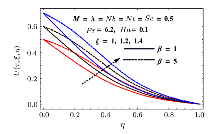
Fig. 2(Color online) Behaviors of $\beta$ and $\xi$ on $U$.

Fig. 3

New window|Download| PPT slide
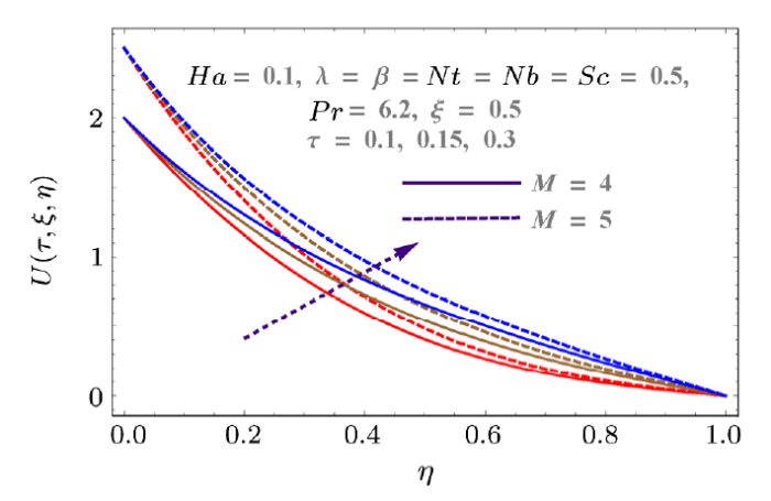
Fig. 3(Color online) Behaviors of $M$ and $\tau$ on $U$.

Fig. 4

New window|Download| PPT slide
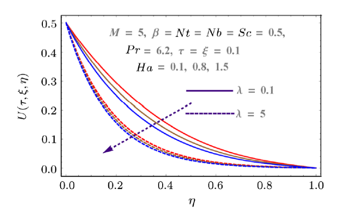
Fig. 4(Color online) Behaviors of $\lambda$ and $Ha$ on $U$.

Fig. 5

New window|Download| PPT slide
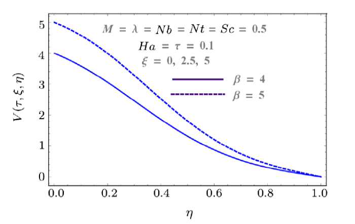
Fig. 5(Color online) Behaviors of $\beta$ and $\xi$ on $V$.

Fig. 6

New window|Download| PPT slide
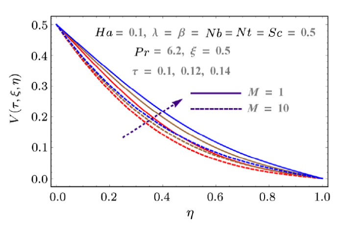
Fig. 6(Color online) Behaviors of $\tau$ and $M$ on $V$.

Fig. 7

New window|Download| PPT slide
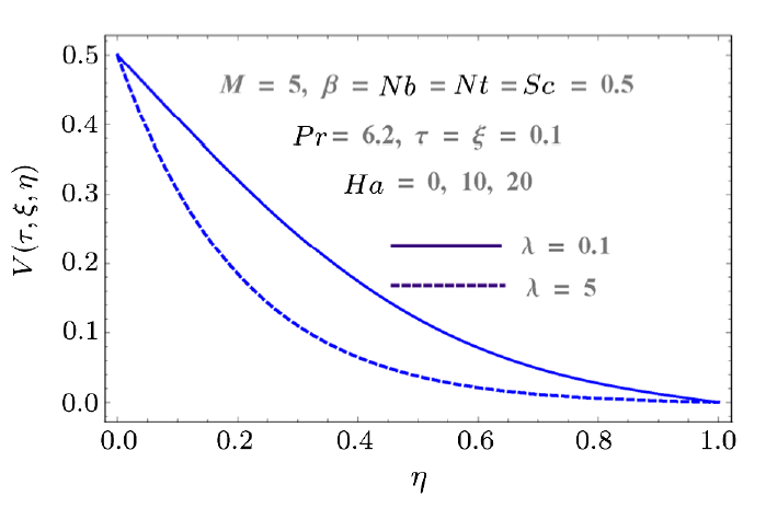
Fig. 7(Color online) Effects of $\lambda$ and $Ha$ on $V$.



Figure 2 shows the impact of injection variable on horizontal component of velocity $U(\tau,\xi,\eta)$. It shows that injection process tends to velocity enhancement due to an increase in boundary layer thickness. Figure 3 is sketched to show the behavior of velocity $U(\tau,\xi,\eta)$ with respect to time as well as Reynolds number $(M)$. Increasing values of Reynolds number produces more turbulence in the flow. This is the reason for more disturbance inside the fluid particles which increases the velocity in x-direction. This figure also shows that velocity increases with time. Impacts of porosity parameter $(\lambda)$ and Hartmann number $(Ha)$ on velocity are portrayed in Fig. 4. Since porosity parameter is inversely proportional to permeability of medium, so more porous medium decreases the speed of fluid particles. Hence velocity decreases. Similarly Hartmann number also decays the velocity due to Lorentz force produced inside the system, which slows the fluid particles. Injection parameter increases the velocity component $V(\tau,\xi,\eta)$ due to injection of more fluid particles inside the system as shown in Fig. 5. Vertical component of velocity $V(\tau,\xi,\eta)$ with respect to material parameter $M$ and time is given in Fig. 6. Stretching is produced in the lower plate, so less disturbance is felt at the upper plate. That is why velocity has a decreasing behavior due to material parameter, while it increases with respect to time. Behaviors of vertical velocity component $V(\tau,\xi,\eta)$ due to Hartmann number $Ha$ and porosity parameter are shown in Fig. 7. Since magnetic field is parallel to velocity component $V(\tau,\xi,\eta)$ so it has no effect on vertical velocity $V(\tau,\xi,\eta)$. However it decreases with respect to porosity parameter because of the decrease in the permeability of medium.

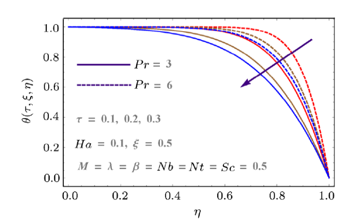
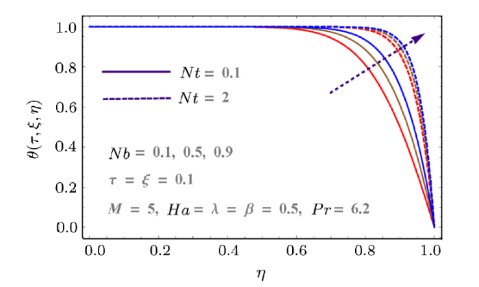
Effects of thermophoresis variable $(Nt)$, Prandtl number $(Pr)$ and Brownian variable $(Nb)$ on temperature $\theta(\tau,\xi,\eta)$ are described in Figs. 8--9. Figure 8 is delineated to show the impact of $Pr$ and time on temperature. Since the lower plate is at higher temperature so temperature of the system gradually decreases with time. However it increases with $Pr$ due to decreases in thermal diffusivity of fluid. As a result the system is heated up which consequently increases the temperature. Figure 9 shows the influences of $Nt$ and $Nb$ on temperature. Here boundary layer thickness increases for larger $Nt$ and $Nb$ and consequently temperature enhances.

Fig. 8

New window|Download| PPT slide
Fig. 8(Color online) Effects of $Pr$ and $\tau$ on $\theta$.

Fig. 9

New window|Download| PPT slide
Fig. 9(Color online) Behaviors of $Nt$ and $Nb$ on $\theta$.



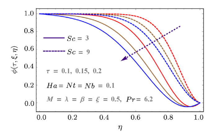
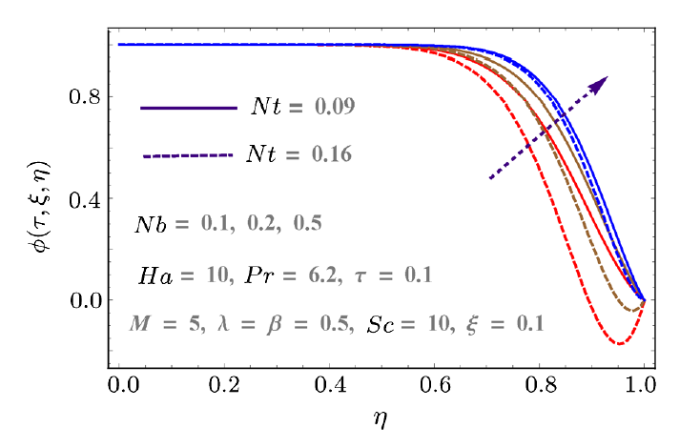
Behaviors of thermophoresis variables $(Nt)$, Schmidt number $(Sc)$ and Brownian parameter $(Nb)$ on concentration $(\phi(\tau,\xi,\eta))$ are disclosed in Figs. 10--11. Effects of $Sc$ and time on $\phi(\tau,\xi,\eta)$ are displayed in Fig. 10. As $Sc$ is the relation of viscous diffusion rate and mass diffusion rate so larger $Sc$ enhances the concentration field. With passing time the concentration show decreasing behavior. Likewise, Fig. 11 is displayed to present the effects of $Nt$ and $Nb$ on $\phi(\tau,\xi,\eta)$. Here concentration field increases for $Nb$ but it decays for thermophoresis parameter $Nt$.

Fig. 10

New window|Download| PPT slide
Fig. 10(Color online) Behaviors of $Sc$ and $\tau$ on $\phi$.

Fig. 11

New window|Download| PPT slide
Fig. 11(Color online) Behaviors of $Nt$ and $Nb$ on $\phi$.



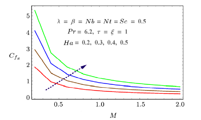
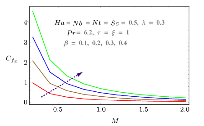
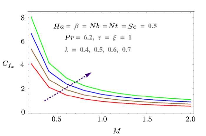
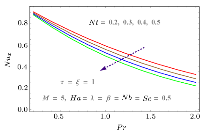
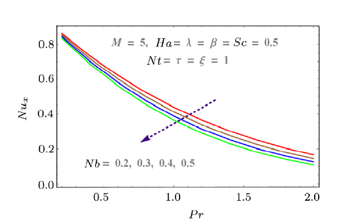
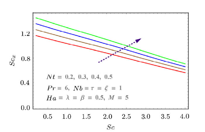
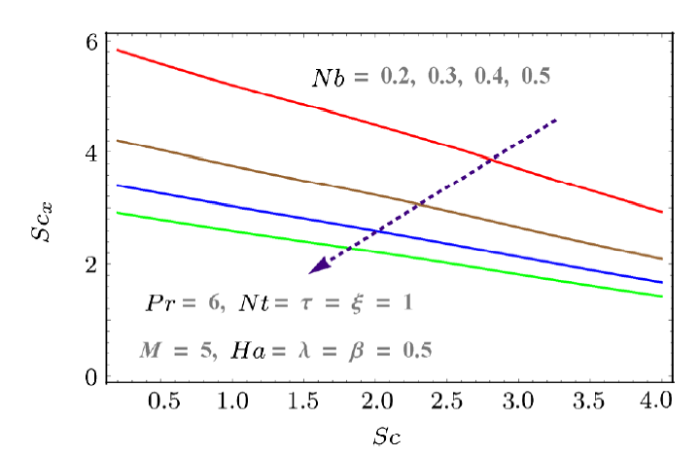
Skin friction, mass and heat transfer rates with respect to pertinent parameters are discussed graphically in Figs. 12--18. Skin friction increases with Hartmann number $Ha$ and Reynolds number $M$. Both parameters result in more resistance to fluid motion. Increasing behavior is observed as shown in Fig. 12. Similarly porosity parameter also increases the drag force (see Fig. 13). Effects of $Nt$ and $Nb$ on heat transfer rate is discussed in Figs. 15 and 16. Larger values of $Nb$ and $Nt$ decrease the temperature difference. That is why $Nu_x$ decreases with both parameters. Similarly mass transfer rate for increasing values of $Nb$ and $Nt$ are given in Figs. 17 and 18. These figures show that mass transfer rate decreases with larger $Nb$ while it increases for $Nt$.

Fig. 12

New window|Download| PPT slide
Fig. 12(Color online) Behaviors of $M$ and $Ha$ on $C_{f_x}$.

Fig. 13

New window|Download| PPT slide
Fig. 13(Color online) Effect of $\beta$ on $C_{f_x}$.

Fig. 14

New window|Download| PPT slide
Fig. 14(Color online) Effect of $\lambda$ on $C_{f_x}$.

Fig. 15

New window|Download| PPT slide
Fig. 15(Color online) Behaviors of $Pr$ and $Nt$ on $Nu_x$.

Fig. 16

New window|Download| PPT slide
Fig. 16(Color online) Effect of $Nb$ on $Nu_x$.

Fig. 17

New window|Download| PPT slide
Fig. 17(Color online) Effects of $Nt$ and $Sc$ on $Sh_x$.

Fig. 18

New window|Download| PPT slide
Fig. 18(Color online) Effects of $Nb$ on $Sh_x$.



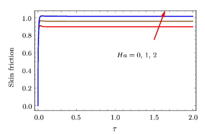
In some limiting case, we draw the effect of magnetic parameter on skin friction in Fig. 19. And the result is compared with Fig. 5 in Ref. ^[20]. Here we found a very good agreement. Therefore the present mathematical model and numerical method is verified.

Fig. 19

New window|Download| PPT slide
Fig. 19(Color online) Impact of magnetic parameter on skin friction.



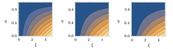
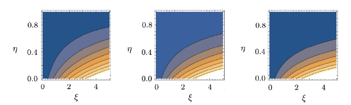
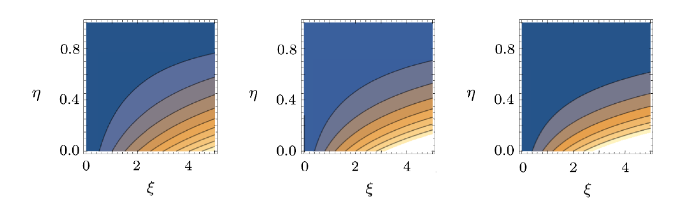
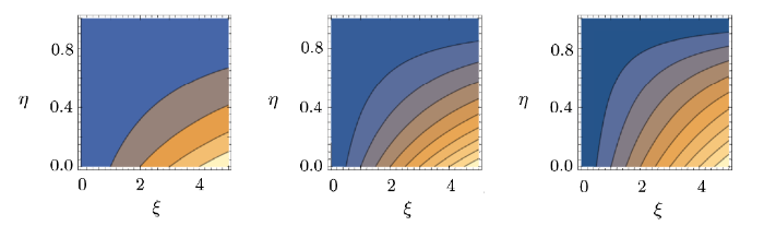
Streamline for the current flow situation are sketched through Figs. 20--23. The number of streamlines in these figures show the velocity of fluid. The more the streamlines, greater is the velocity of fluid. Figures 20--22 show that velocity decreases with Reynolds number $(M)$, porosity parameter $(\lambda)$ and Hartmann number $(Ha)$ while it increases with injection parameter $(\beta)$ (see Fig. 23).

Fig. 20

New window|Download| PPT slide
Fig. 20(Color online) Streamlines for $M=1$, 1.5, 3.

Fig. 21

New window|Download| PPT slide
Fig. 21(Color online) Streamlines for $Ha=1$, 2, 3.

Fig. 22

New window|Download| PPT slide
Fig. 22(Color online) Streamlines for $\lambda=1$, 2, 3.

Fig. 23

New window|Download| PPT slide
Fig. 23(Color online) Streamlines for $\beta=1$, 2, 5.

6 Conclusions

In this paper, we studied flow of viscous nanofluid between stretchable parallel plates in porous medium. The governing PDE's system is transformed to dimensionless form by dimensionless parameters. For solution we used Numerical technique i.e. Finite difference scheme. From the results we obtained that velocity increases through Reynolds number and injection parameters while it reduces with magnetic and porosity parameters. Temperature $(\theta(\tau,\xi,\eta))$ increases for larger Brownian variable $(Nb)$, Prandtl number $(Pr)$, and thermophoresis variable $(Nt)$. Concentration $(\phi(\tau,\xi,\eta))$ increases for larger Schmidt number and Brownian motion while it decays with thermophoresis parameter. Skin friction increases with Hartmann number, injection parameter and porosity parameter. Sherwood number increases with $Nt$ and decreases for $Nb$ and $Sc$.

Reference View Option By original order
By published year
By cited within times
By Impact factor

[1] S. U. S. Choi , ASME FED 66 ( 1995) 99.
[Cited within: 1]

[2] J. Buongiorno , ASME J. Heat Transf. 128 ( 2006) 240.
[Cited within: 1]

[3] S. Ahmad, M. I. Khan, T. Hayat , et al., Coll. Surf. A: Phys. Eng. Asp. 554 ( 2018) 197.
[Cited within: 1]

[4] M. Sheikholeslami, H. R. Kataria, A. S. Mittal , J. Mol. Liq. 257 ( 2018) 12.


[5] R. Ahmad, M. Mustafa, M. Turkyilmazoglu , Int. J. Heat Mass Transfer. 111 ( 2017) 827.


[6] T. Hayat, M. I. Khana, T. A. Khand , et al., J. Mol. Liq. 265 ( 2018) 629.


[7] T. Hayat, S. Ahmad, M. I. Khan, A. Alsaedi , Results Phys. 8 ( 2018) 34.


[8] T. Hayat, S. Ahmad, M. I. Khan, A. Alsaedi , Commun. Theor. Phys. 69 ( 2018) 569.
[Cited within: 1]

[9] M. Turkyilmazoglu , Comput. Fluid. 94 ( 2014) 139.
[Cited within: 1]

[10] M. Sheikholeslami, M. Hatami, D. D. Ganji , J. Mol. Liq. 211 ( 2015) 577.
[Cited within: 1]

[11] K. R. Rajagopal, T. Y. Na, A. S. Gupta , Rheol. Acta 23 ( 1984) 213.
[Cited within: 1]

[12] D. F. Fairbank and C. R. Wike , Ind. Eng. Chem. Res. 42 ( 1950) 471.
[Cited within: 1]

[13] N. Riley , J. Fluid Mech. 18 ( 1964) 577.
[Cited within: 1]

[14] H. I. Andersson, O. R. Hansen, B. Holmedal , Int. J. Heat. Mass Transf. 37 ( 1994) 659.
[Cited within: 1]

[15] T. Hayat, S. Ahmad, M. I. Khan, A. Alsaedi , Results Phys. 8 ( 2018) 545.
[Cited within: 1]

[16] E. Magyari and B. Keller , Eur. J. Mech. B. Fluids 19 ( 2000) 109.
[Cited within: 1]

[17] E. Magyari and B. Keller , Int. J. Thermal Sci. 44 ( 2005) 245.
[Cited within: 1]

[18] Z. H. Khan, O. D. Makinde, R. Ahmad, W. A. Khan , Commun. Theor. Phys. 70 ( 2018) 641.
[Cited within: 1]

[19] R. Abreu, Z. Su, J. Kamm, J. Gao , J. Comp. Appl. Math. 340 ( 2018) 390.


[20] O. D. Makinde, Z. H. Khan, R. Ahmad, W. A. Khan , Phys. Fluids 30 ( 2018); doi: https://ctp.itp.ac.cn/article/2019/0253-6102/10.1063/1.5046331.
[Cited within: 2]