Malik Zaka Ullah^,1,*, Metib Alghamdi²1 Department of Mathematics, Faculty of Science, King Abdulaziz University, Jeddah 21589, Saudi Arabia
2 Department of Mathematics, Faculty of Science, King Khalid University, Abha 61413, Saudi Arabia

Corresponding authors: *E-mail:malikzakas@gmail.com

Received:2019-03-28Online:2019-12-1


Abstract
In this paper, the magnetohydrodynamic 3D flow of Prandtl nanoliquid subject to convectively heated extendable surface has been discussed. A linear stretching surface makes the flow. Thermophoretic and Brownian motion impacts are explored. Heat transfer for convective procedure is considered. Prandtl liquid is taken electrically conducted through applied magnetic field. Suitable non-dimensional variables lead to strong nonlinear ordinary differential system. The obtained nonlinear differential systems are solved through optimal homotopic technique. Physical quantities like skin friction coefficients and Nusselt number are explored via plots. It is observed that effects of Hartman parameter and Biot number on temperature and concentration are quite similar. Both temperature and concentration are enhanced for larger values of Hartman parameter and Biot number.
Keywords： three-dimensional flow;MHD;Prandtl fluid;nanoparticles;optimal homotopy analysis method (OHAM)


PDF (383KB)MetadataMetricsRelated articlesExportEndNote|Ris|BibtexFavorite
Cite this article
Malik Zaka Ullah, Metib Alghamdi. An Optimal Analysis for 3D Flow of Prandtl Nanofluid with Convectively Heated Surface. [J], 2019, 71(12): 1485-1492 doi:10.1088/0253-6102/71/12/1485

1 Introduction

Nanomaterials considered a main factor in industry development. Nanofluids are an important branch of nanomaterials, which were firstly referred by Choi^[1] in $1995$. Nanofluids are identified as a base fluid contains suspended small particles (1$-$100) nm. Water, oil, and alcohols are commonly base fluids. The importance of nanofluids is due to their unusual thermophysical properties. Nanofluids exhibit high ability to conduct electricity and heat, so it plays a vital role in industry. Before long nanofluid components have expanded vital centralization of researchers inferable from their entrancing warm transport in a couple of calm disapproved of fields. There are many applications such as engine cooling, cooling of electronics, refrigeration, solar water heating, microprocessors, laser applications and super conducting magnets. Jang and Choi^[2] discussed the role of Brownian motion in the enhanced thermal conductivity of nanofluids. After that Brownian dynamics simulation to determine the effective thermal conductivity of nanofluids is reported by Bhattacharya $et$ $al.$^[3] Buongiorno^[4] presented complete model to analyze the aspects of thermophoresis and Brownian motion. Some continuous explores on nanofluid stream subject can be directed through the examinations.^[5-30]

Flow of liquid on stretching sheet is now massively acknowledge by the researchers because of their large engineering and industrial application in rubber sheets, manufacture of food, glass fiber, hot rolling, paper production and many others. However liquid flow due to non-linear stretching sheet is scare. Rahimi $et$ $al.$^[31] considered collocation method to explore the solutions of an Eyring-Powell fluid caused by linear stretching sheet. Combined properties of viscous dissipation and MHD on the micropolar nanofluid on stretching sheet have been examined by Hsiao.^[32] Zhang $et$ $al.$^[33] analyzed the unsteady flow of Oldroyd-B nanofluid because of stretching sheet. Hayat $et$ $al.$^[34] investigated stretched flow of Jeffery fluid. Recently researchers have investigated the flow of non-Newtonian and Newtonian liquids over non-linear stretching sheet. Seth and Mishra^[35] used the Navier's slip condition to study the transient flow of nanofluid past a non-linear stretching sheet. Hussain $et$ $al.$^[36] studied the characteristics of tangent hyperbolic fluid along non-linear stretching sheet by using convective boundary conditions. Hayat $et$ $al.$^[37] explored the non-linear stretched flow of second grade fluid. Nanofluid flow with variable thickness comprising electrical MHD in the non-linear stretched sheet is discussed by Daniel $et$ $al.$^[38]

Magnetohydrodynamic is the study of magnetic behavior in electrically conducting fluids. Plasmas, salt water and liquid metals are examples of such fluids. In Physics, Hannes Alfvén achieved Nobel Prize in $1970$ for his great work on MHD. Magnetohydrodynamic is important in astrophysics, space plasma physics, cancer tumor treatment, solar physics, blood pump machine, and laboratory plasma experiments. Ishak $et$ $al.$^[39] considered MHD flow past a radially shrinking or stretching disk. Huang and Liu^[40] attempted to combine fluid hammer effect with MHD effect. Hayat $et$ $al.$^[41] computed numerical results for MHD flow with Soret and Dufour effects. Hayat $et$ $al.$^[42] studied three-dimensional flow due to exponentially stretching surface in the existence of an applied magnetic field and Joule heating effects. Second grade nanofluid with MHD over a nonlinear stretching surface is studied by Hayat $et$ $al.$^[43] Tamoor $et$ $al.$^[44] discussed MHD Casson flow between stretching cylinder.

The prime purpose of present topic is to illustrate hydromagnetic 3D stream of Prandtl liquid^[45-48] inside seeing nanoparticles. Thermal and mass trade properties are portrayed through random spread and thermophoresis. Prandtl liquid is taken driving through uniform associated alluring field. Thermal convective condition^[49-50] and a condition related with zero nanoparticles change^[51-52] are completed at the farthest point. The obtained nonlinear differential systems are solved through optimal homotopic analysis method (OHAM).^[53-59] Effects of a couple of physical variables are inspected. In addition the coefficients of surface drag and warmth conversion standard are explored graphically.

2 Formulation

We inspect steady hydromagnetic three-dimensional (3D) flow of Prandtl nanoliquid by a linear deformable surface. Thermal condition and as of late made necessity are requiring zero nanoparticles movement are constrained at the point of confinement. Brownian advancement and thermophoretic effects are investigated. The fluid is assumed to be conducted electrically with magnetic field $B_{0}$ applied parallel to $z$-direction. For very small Reynolds number\ current hall and magnetic field effects are ignored. Cartesian coordinate system is incorporated. The sheet is stretched along $x$- and $y$-directions at $z=0$ with velocities $U_{w}$ and $V_{w}$. Boundary layer expressions governing the flow of Prandtl nanofluid in the absence of viscous dissipation and thermal radiation are written as follows:^[16,48]

(1) $$ \frac{\partial u}{\partial x}+\frac{\partial v}{\partial y}+\frac{\partial w}{\partial z}=0\,, $$
(2) $$ u\frac{\partial u}{\partial x}+v\frac{\partial u}{\partial y}+w\frac{\partial u}{\partial z}=\nu \frac{A}{c}\frac{\partial ^{2}u}{\partial z^{2}} \nonumber\\ \quad +\frac{\nu A}{2c^{3}}\left( \frac{\partial u}{\partial z}\right) ^{2}\frac{\partial ^{2}u}{\partial z^{2}}-\frac{\sigma B_{0}^{2}}{\rho _{f}}u\,, $$
(3) $$ u\frac{\partial v}{\partial x}+v\frac{\partial v}{\partial y}+w\frac{\partial v}{\partial z}=\nu\frac{A}{c}\frac{\partial ^{2}v}{\partial z^{2}} \nonumber\\ \quad +\frac{\nu A}{2c^{3}}\left( \frac{\partial v}{\partial z}\right) ^{2}\frac{\partial ^{2}v}{\partial z^{2}}-\frac{\sigma B_{0}^{2}}{\rho _{f}}v\,, $$
(4) $$ u\frac{\partial T}{\partial x}+v\frac{\partial T}{\partial y}+w\frac{\partial T}{\partial z}=\alpha ^{\star }\frac{\partial ^{2}T}{\partial z^{2}} \nonumber\\ \quad +\frac{(\rho c)_{p}}{\left( \rho c\right) _{f}}\left( D_{B}\left( \frac{\partial T}{\partial z}\frac{\partial C}{\partial z}\right)+\frac{D_{T}}{T_{\infty }}\left( \frac{\partial T}{\partial z}\right) ^{2}\right), $$
(5) $$ u\frac{\partial C}{\partial x}+v\frac{\partial C}{\partial y}+w\frac{\partial C}{\partial z}=D_{B}\left( \frac{\partial ^{2}C}{\partial z^{2}}\right) \nonumber\\ \quad +\frac{D_{T}}{T_{\infty }}\left( \frac{\partial ^{2}T}{\partial z^{2}}\right). $$
Here one has the following conditions:^[16,48]

(6) $$ u=U_{w}=ax,\quad v=V_{w}=by,\quad w=0\,, \nonumber -k\frac{\partial T}{\partial z}=h_{f}\left( T_{f}-T\right) \,, D_{B}\frac{\partial C}{\partial z} +\frac{D_{T}}{T_{\infty }}\frac{\partial T}{\partial z}=0 {\rm at} z=0\,, \\ $$
(7) $$ u\rightarrow 0,\;\; v\rightarrow 0,\;\; T\rightarrow T_{\infty },\;\; C\rightarrow C_{\infty }\;\; {\rm as} z\rightarrow\infty\,. $$
Here $u$, $v$, and $w$ speak to the speeds in $x$-, $y$-, and $z$-bearings, $\mu$ the dynamic consistency, $\nu\left( =\mu /\rho _{f}\right)$ the kinematic thickness, $k$ the warm conductivity, $\rho _{f}$ the thickness, $A$ and $c$ the material constants of Prandtl fluid model,$\sigma $ the electrical conductivity, $\alpha ^{\star }=k/(\rho c)_{f}$ the warm diffusivity, $(\rho c)_{f}$ the warmth capability of the fluid, $(\rho c)_{p} $ the powerful warmth capability of nanoparticles, $T$ the temperature, $D_{B}$ the Brownian development, $C$ the focus, $D_{T}$ the thermophoretic dispersion and $T_{\infty }$ and $C_{\infty }$ the encompassing liquid temperature and fixation. Considering

(8)$ u\!=\!axf^{\prime }(\zeta ),\quad v\!=\!ayg^{\prime }(\zeta ),\quad w\!=\!-\!\left(a\nu \right) ^{1/2}(f\left( \zeta \right) \!+\!g(\zeta )),\quad \nonumber \theta (\zeta )\!=\!\frac{T-T_{\infty }}{T_{f}-T_{\infty }},\quad \phi (\zeta )\!=\!\frac{C-C_{\infty }}{C_{\infty }},\quad \zeta \!=\!\left( \frac{a}{\nu }\right)^{1/2}z.$
Expression $(1)$ is naturally fulfilled and Eqs. (2)$-$(7) have the accompanying structures

(9) $$ \beta _{1}f^{\prime \prime \prime }+(f+g)f^{\prime \prime }-f^{\prime2}+\beta _{2}f^{\prime \prime ^{2}}f^{\prime \prime \prime}-(Ha)^{2}f^{\prime }=0, $$
(10) $$ \beta _{1}g^{\prime \prime \prime }+(f+g)g^{\prime \prime }-g^{\prime 2}+\beta _{2}g^{\prime \prime ^{2}}g^{\prime \prime \prime }-(Ha)^{2}g^{\prime }=0, $$
(11) $$ \theta^{\prime \prime }+Pr\left((f+g)\theta^{\prime }+N_{b}\theta^{\prime }\phi^{\prime }+N_{t}\theta^{\prime 2}\right)=0, $$
(12) $$ \phi^{\prime \prime }+Sc(f+g)\phi ^{\prime }+\frac{N_{t}}{N_{b}}\theta^{\prime \prime }=0, $$
(13) $$ f(0)=g(0)=0,\quad f^{\prime }(0)=1,\quad g^{\prime }(0)=\alpha,\quad \nonumber \theta^{\prime }(0)=-\gamma (1-\theta (0)),\quad N_{b}\phi^{\prime}(0)+N_{t}\theta^{\prime }(0)=0, $$
(14) $$ f^{\prime }(\infty )\rightarrow 0,\quad g^{\prime }(\infty )\rightarrow 0,\quad \theta (\infty )\rightarrow 0,\quad \phi (\infty )\rightarrow 0. $$
Here $\beta _{1}$ remains for Prandtl fluid number, $\beta _{2}$ for flexible number, $Ha$ for Hartman parameter, $\alpha $ for ratio parameter, $%Pr$ for Prandtl number, $\gamma $ for Biot number, $N_{b}$ for Brownian development parameter, $N_{t}$ for thermophoresis number and $Sc$ for Schmidt number. These parameters are characterized by:

(15) $$ \beta _{1}=\frac{1}{\mu Ac},\quad \beta _{2}=\frac{bU_{w}}{2c^{2}\nu},\quad (Ha)^{2}=\frac{\sigma B_{0}^{2}}{a\rho _{f}},\quad \nonumber\\ \alpha =\frac{b}{a},\quad \gamma =\frac{h_{f}}{k}\sqrt{\frac{\nu }{a}},\quad N_{b}=\frac{\left( \rho c\right) _{p}D_{B}C_{\infty }}{\left( \rho c\right)_{f}\nu },\quad \nonumber\\ N_{t}=\frac{\left( \rho c\right) _{p}D_{T}\left(T_{f}-T_{\infty }\right) }{\left( \rho c\right) _{f}\nu T_{\infty }},\quad \nonumber\\ Pr=\frac{\nu }{\alpha ^{\star }},\quad Sc=\frac{\nu }{D_{B}}. $$
The physical quantities are given by

(16) $$ Re_{x}^{1/2}C_{f}=\left( \beta _{1}f^{\prime \prime }(0)+\beta_{2}f^{\prime \prime }(0)^{3}\right) ,\quad \nonumber\\ Re_{y}^{1/2}C_{g}=\left( \beta _{1}g^{\prime \prime}(0)+\beta _{2}g^{\prime \prime }(0)^{3}\right) ,\quad \nonumber\\ Re_{x}^{-1/2}Nu_{x}=-\theta ^{\prime }\left( 0\right) . $$
It is seen that mass motion spoken to by Sherwood number is presently indistinguishably evaporates and $Re_{x}$=$U_{w}x/\nu$ and $Re_{y}$=$V_{w}y/\nu$ delineate nearby Reynolds parameters. It is also noticed that the Prandtl fluid model reduces to viscous fluid case when $\beta_{1}=1$ and $\beta _{2}=0.$

3 OHAM Solutions

It has been noted that Eqs. (9)--(12) along with boundary conditions (13) and (14) are four non-linear ordinary differential equations whose optimal series arrangements have been developed by employing OHAM. The initial deformations ($f_{0}$, $g_{0}$, $\theta _{0}$, $\phi _{0}$) and auxiliary linear operators ($\mathcal{L}_{f}$, $\mathcal{L}_{g}$, $\mathcal{L}_{\theta},\mathcal{L}_{\phi }$) are

(17) $$ f_{0}(\zeta )=1-e^{-\zeta },\quad g_{0}(\zeta )=\alpha (1-e^{-\zeta }),\quad \nonumber\\ \theta _{0}(\zeta )=\frac{\gamma }{1+\gamma }e^{-\zeta },\quad \phi _{0}(\zeta )=-\frac{\gamma }{1+\gamma }\frac{N_{t}}{N_{b}}e^{-\zeta }, $$
(18) $$ \mathcal{L}_{f}=f^{\prime \prime \prime }-f^{\prime },\quad \mathcal{L}_{g}=g^{\prime \prime \prime }-g^{\prime },\quad \nonumber\\ \mathcal{L}_{\theta}=\theta ^{\prime \prime }-\theta ,\quad \mathcal{L}_{\phi }=\phi^{\prime \prime }-\phi . $$
The above linear operators obey

(19) $$ \mathcal{L}_{f}\left[ H_{1}^{\star \ast }+H_{2}^{\star \ast }e^{\zeta}+H_{3}^{\star \ast }e^{-\zeta }\right] =0,\quad \nonumber\\ \mathcal{L}_{g}\left[H_{4}^{\star \ast }+H_{5}^{\star \ast }e^{\zeta }+H_{6}^{\star \ast}e^{-\zeta }\right] =0,\quad \nonumber \mathcal{L}_{\theta }\left[ H_{6}^{\star \ast }e^{\zeta }+H_{7}^{\star \ast}e^{-\zeta }\right] =0,\quad \nonumber\\ \mathcal{L}_{\phi }\left[ H_{8}^{\star\ast }e^{\zeta }+H_{9}^{\star \ast }e^{-\zeta }\right] =0, $$
in which $H_{j}^{\star \ast }$ ($j$ = 1$-$10) illustrate the arbitrary constants. The zeroth and $m$-th order deformation problems can be easily defined in view of above operators via BVPH$2.0$ of software $Mathematica$.

4 Convergence Analysis

We have unwound the power, essentialness and center verbalizations with the help of BVPh2.0. These verbalizations contain cloud factors $\hbar _{f}$, $\hbar _{g}$, $\hbar _{\theta }$, and $\hbar _{\phi }$. We can process the base estimation of these elements by taking total mix-up pretty much nothing. In the packaging of HAM, these elements expect a basic employment.That is the reason these variables insinuate as association control parameter, which shifts HAM from other illustrative conjecture systems. With a particular ultimate objective to diminish the CPU time, we have used typical waiting errors at the $m$-th order of theory which are described by

(20) $$ \varepsilon _{m}^{f}=\frac{1}{k+1}\sum\limits_{j=0}^{k}\left[\mathcal{N}_{f}\left(\sum\limits_{i=0}^{m}\hat{f}\left( \zeta \right),\sum\limits_{i=0}^{m}\hat{g}\left(\zeta\right)\right) _{\zeta =j\delta\zeta }\right] ^{2}, $$
(21) $$ varepsilon _{m}^{g}=\frac{1}{k+1}\sum\limits_{j=0}^{k}\left[ \mathcal{N}_{g}\left( \sum\limits_{i=0}^{m}\hat{f}\left( \zeta \right),\sum\limits_{i=0}^{m}\hat{g}\left( \zeta \right) \right) _{\zeta =j\delta\zeta }\right] ^{2}, $$
(22) $$ \varepsilon _{m}^{\theta }=\frac{1}{k+1}\sum\limits_{j=0}^{k}\left[\mathcal{N}_{\theta }\left( \sum\limits_{i=0}^{m}\hat{f}\left( \zeta\right) ,\sum\limits_{i=0}^{m}\hat{g}\left( \zeta \right),\sum\limits_{i=0}^{m}\hat{\theta}\left( \zeta \right),\sum\limits_{i=0}^{m}\hat{\phi}\left( \zeta \right) \right) _{\zeta=j\delta \zeta }\right] ^{2}, $$
(23) $$ \varepsilon _{m}^{\phi }=\frac{1}{k+1}\sum\limits_{j=0}^{k}\left[ \mathcal{N}_{\phi }\left( \sum\limits_{i=0}^{m}\hat{f}\left(\zeta \right),\sum\limits_{i=0}^{m}\hat{g}\left(\zeta \right),\sum\limits_{i=0}^{m}\hat{\theta}\left( \zeta \right),\sum\limits_{i=0}^{m}\hat{\phi}\left(\zeta \right) \right) _{\zeta =j\delta \zeta }\right] ^{2}. $$
Here $\mathcal{N}_{f}$, $\mathcal{N}_{g}$, $\mathcal{N}_{\theta }$, and $\mathcal{N}_{\phi }$ denote the non-linear operators corresponding to Eqs. (9)--(12) respectively. Following Liao:^[53]

(24) $$ \varepsilon_{m}^{t}=\varepsilon _{m}^{f}+\varepsilon _{m}^{g}+\varepsilon_{m}^{\theta }+\varepsilon _{m}^{\phi }, $$
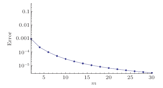
where $\varepsilon_{m}^{t}$ indicates add up to leftover squared blunder,$k=20$ and $\delta \zeta=0.5$. Ideal information for assistant parameters at second request of approximations is $\hbar_{f}=-1.591 89$, $\hbar_{g}=-3.056 54$,$\hbar_{\theta }=-1.365 14$, $\hbar _{\phi }=-1.186 26$ and $\varepsilon_{m}^{t}=9.39\times10^{-4}$. Figure 2 speaks to related aggregate remaining mistake plot. Table 1 illustrates normal square residual errors. It has been dissected that the normal averaged square errors decrease with higher request disfigurements.

New window|Download| PPT slide
Fig. 1Total residual error plot.




Table 1
Table 1Averaged normal residual square errors utilizing ideal information of helper factors.

New window|CSV

New window|Download| PPT slide
Fig. 2variation for $\beta _{1}$.

5 Graphical Results and Discussion

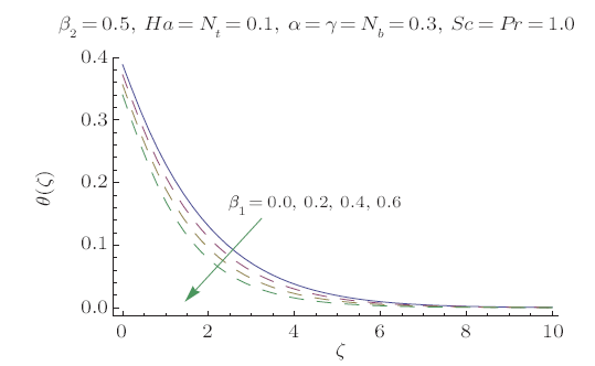
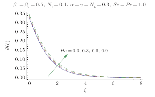
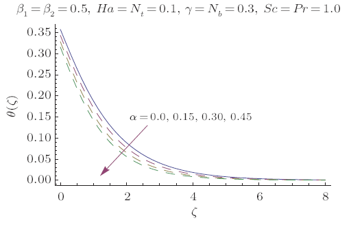
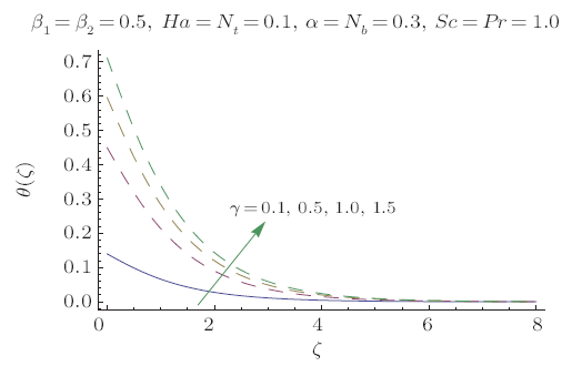
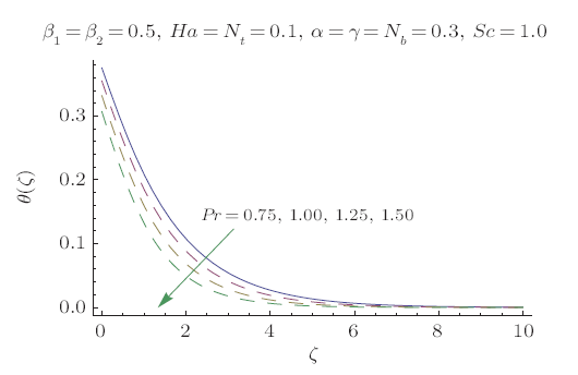
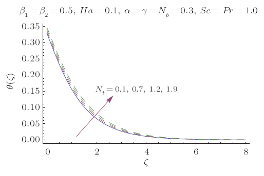
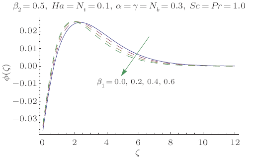
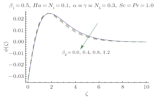
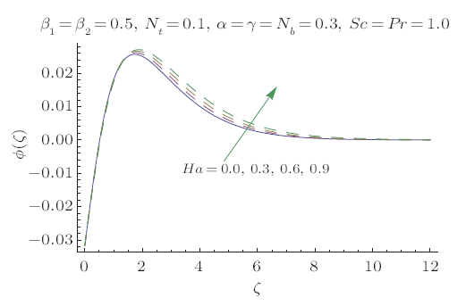
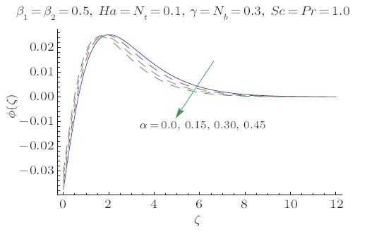
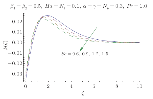
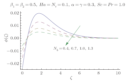
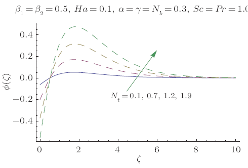
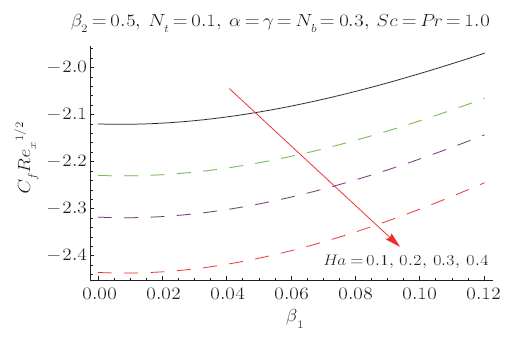
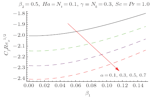
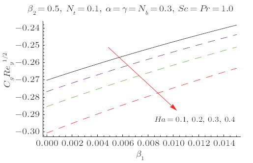
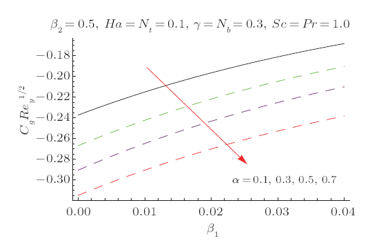
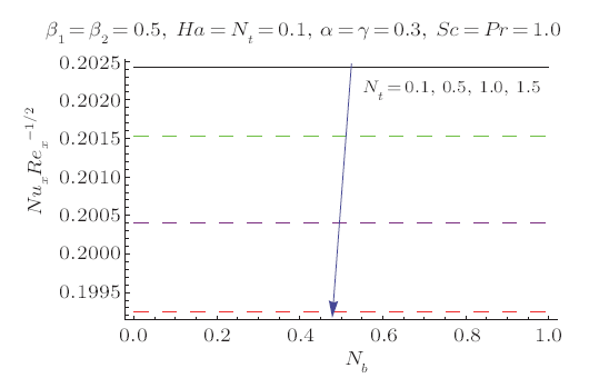
This section researches impacts of two or three significant physical stream factors like Prandtl liquid parameter $\beta _{1}$, adaptable parameter $\beta _{2}$, Hartman number $Ha$, extent number $\alpha $, Biot parameter $\gamma $, Prandtl parameter $Pr$, Schmidt parameter $Sc$, Brownian improvement parameter $N_{b}$ and thermophoresis number $N_{t}$ on temperature $\theta (\zeta )$ and focus $\phi (\zeta )$. Figures 2 and 3 are constructed to present $\theta (\zeta )$ for different estimations of $\beta _{1}$ and $\beta _{2}$. It is noted from these figures that increase in $\beta _{1}$ and $\beta _{2}$ leads to decrease in temperature. Figure 4 displays the variations of Hartman number $Ha$ on temperature profile $\theta (\zeta )$. Lorentz force arises in $Ha$ that resists the fluid motion therefore temperature field $\theta (\zeta )$ enhances. Figure 5 demonstrates that an adjustment in extent number $\alpha $ prompts a poor temperature $\theta (\zeta )$ and less layer of warm. Impact of Biot number $\gamma $ on $\theta (\zeta )$ is depicted in Fig. 6. Increase in $\gamma $ causes a powerful convection that display an increment in $\theta (\zeta )$. Figure 7 shows that temperature diminish for greater values of Prandtl number. As greater $Pr$ corresponds to lower thermal diffusivity $\alpha $ which causes decrease in temperature. Figure 8 is constructed to study the influence of thermophoresis parameter on the temperature field. This figure illustrates that increase in thermophoresis $N_{t}$ parameter tends to higher temperature. This parameter is occurred due to nanomaterials. The existence of nanomaterials raised the thermal conductivity of nanoliquids. Nanofluid thermal conductivity is an increasing function of temperature. That is why enhancement in temperature is observed for greater estimation of $N_{t}$. Figures 9 and 10 elucidate that nanoparticles concentration is smaller for greater values of $\beta _{1}$ and $\beta _{2}$ (material parameters). Figures 11 and 12 are plotted to analyze the change in $\phi \left( \zeta \right) $ for larger Hartman number and extent parameter $\alpha $. We observed that increasing and decaying impacts occur for both dimensionless parameters on concentration profile. Figure 13 shows the consequences of Schmidt number on $\phi \left( \zeta \right) .$ Schmidt number relates to the mass diffusion of a system. As $Sc$ is increased mass diffusion decreases due to which concentration shows decreasing trend. Brownian parameter $N_{b}$ when increased causes a change in the Brownian motion of nanoparticles which reduces the distribution of concentration as depicted by Fig. 14. Increasing $N_{t}$ causes increase in thermal conductivity of the system which contributes in increase of concentration as seen in Fig. 15. Figure 16 presents impact of $Ha$ and $\beta _{1}$ on $C_{f}Re_{x}^{1/2}$. It has been seen that $C_{f}Re_{x}^{1/2}$ improves for $Ha$. Figure 17 demonstrates the effects of $\alpha $ and $\beta _{1}$ on $C_{f}Re_{x}^{1/2}$. Obviously $C_{f}Re_{x}^{1/2}$ demonstrates expanding conduct for $\alpha$ and $\beta _{1}$. Figure 18 demonstrates the impacts of $Ha$ and $\beta _{1}$ on $C_{g}Re_{y}^{1/2}$. An upgrade in $Ha$ indicates expanding conduct for $C_{g}Re_{y}^{1/2}$. Figure 19 demonstrates the impacts of $\alpha$ and $\beta_{1}$ on $C_{g}Re_{y}^{1/2}$. From this Figure it has been broke down that $C_{g}Re_{y}^{1/2}$ is a hoisting capacity of $\alpha$. Impact of $N_{b}$ and $N_{t}$ on $Nu_{x}Re_{x}^{1/2}$ are uncovered through Fig. 20. Here $Nu_{x}Re_{x}^{1/2}$ diminishes for $N_{t}$ while steady pattern is seen for $N_{b}$. Table 2 shows the comparison for different values of $\alpha $ with homotopy perturbation method (HPM) and exact solutions. Table 2 presents an excellent agreement of OHAM solutions with the existing homotopy perturbation method (HPM) and exact solutions in a limiting sense.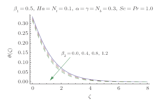

New window|Download| PPT slide
Fig. 3variation for $\beta _{2}$.

New window|Download| PPT slide
Fig. 4variation for $Ha$.

New window|Download| PPT slide
Fig. 5variation for $\alpha $.

New window|Download| PPT slide
Fig. 6variation for $\gamma $.

New window|Download| PPT slide
Fig. 7variation for $Pr$.

New window|Download| PPT slide
Fig. 8variation for $N_{t}$.

New window|Download| PPT slide
Fig. 9variation for $\beta _{1}$.

New window|Download| PPT slide
Fig. 10variation for $\beta _{2}$.

New window|Download| PPT slide
Fig. 11variation for $Ha$.

New window|Download| PPT slide
Fig. 12variation for $\alpha $.

New window|Download| PPT slide
Fig. 13variation for $Sc$.

New window|Download| PPT slide
Fig. 14variation for $N_{b}$.

New window|Download| PPT slide
Fig. 15variation for $N_{t}$.

New window|Download| PPT slide
Fig. 16Plots of $C_{f}{Re}_{x}^{1/2}$ via $Ha$ and $\beta_{1}$.

New window|Download| PPT slide
Fig. 17Plots of $C_{f}{Re}_{x}^{1/2}$ via $\alpha $ and $\beta _{1}$.

New window|Download| PPT slide
Fig. 18Plots of $C_{g}{Re}_{y}^{1/2}$ via $Ha$ and $\beta _{1}$.

New window|Download| PPT slide
Fig. 19Plots of $C_{g}{Re}_{y}^{1/2}$ via $\alpha $ and $\beta _{1}$.

New window|Download| PPT slide
Fig. 20Plots of $Nu_{x}{Re}_{x}^{-1/2}$ via $N_{b}$ and $N_{t}$.




Table 2
Table 2Comparative values of $-f'{}'$(0) and $-g'{}'$(0) for several values of $\alpha$ when $\beta_1=1$ and $\beta_2=Ha =0$.

New window|CSV

6 Conclusions

Here hydromagnetic 3D limit layer stream of Prandtl nanoliquid as a result of straightly deformable surface with convective surface condition is performed. Genuine consequences of the current analysis are sketched out as seeks after:

$\bullet$ Both temperature $\theta (\zeta )$ and fixation $\phi (\zeta )$ fields show decaying design for higher Prandtl liquid $\beta _{1}$ and adaptable $\beta _{2}$ parameters.

$\bullet$ An expansion in Hartman number $Ha$ demonstrates more grounded temperature $\theta (\zeta )$ and fixation $\phi (\zeta )$ fields.

$\bullet$ Higher proportion number $\alpha $ delineate lessening conduct for concentration $\phi (\zeta )$ and temperature $\theta (\zeta )$ fields.

$\bullet$ Higher Biot number $\gamma $ indicates more grounded temperature $\theta (\zeta )$ field.

$\bullet$ Similar behavior is observed for different values of $N_{t}$ on concentration $\phi (\zeta )$ and temperature $\theta (\zeta )$ fields.

$\bullet$ For higher estimations of Prandtl parameter $Pr$, temperature $\theta(\zeta )$ decreases.

$\bullet$ An increment in Schmidt number $Sc$ yields weaker Concentration $\phi(\zeta )$ field.

Concentration $\phi (\zeta )$ field exhibits decaying trend via Brownian advancement number $N_{b}$.

Reference View Option By original order
By published year
By cited within times
By Impact factor

[1] S. U. S . Choi, Enhancing thermal conductivity of fluids with nanoparticles, USA, ASME, FED 231/MD, 66(1995) 99-105.
[Cited within: 1]

[2] S.P Jang .and S. U.S. Choi, Appl. Phys. Lett. 84(2004) 4316.
[Cited within: 1]

[3] P. Bhattacharya, S. K. Saha, A. Yadav, P. E. Phelan, J. Appl. Phys . 95(2004) 6492.
[Cited within: 1]

[4] J. Buongiorno , J. Heat Transfer 128 ( 2006) 240.
[Cited within: 1]

[5] R.K Tiwari .and M. K. Das, Int. J. Heat Mass Transf. 50(2007) 2002.
DOI:10.1016/j.ijheatmasstransfer.2006.09.034URL [Cited within: 1]

[6] S. Kakac and A. Pramuanjaroenkij, Int. J. Heat Mass Transf. 52(2009) 3187.
DOI:10.1016/j.ijheatmasstransfer.2009.02.006URL

[7] E. Abu-Nada and H. F. Oztop , Int. J. Heat Fluid Flow 30 ( 2009) 669.


[8] M. Mustafa, T. Hayat, I. Pop, S. Asghar, S. Obaidat , Int. J. Heat Mass Transfer 54 ( 2011) 5588.


[9] M. Turkyilmazoglu , Chem. Eng. Sci. 84(2012) 182.
DOI:10.1016/j.ces.2012.08.029URL

[10] M. Turkyilmazoglu and I. Pop, Int. J. Heat Mass Transf. 59(2013) 167.
DOI:10.1016/j.ijheatmasstransfer.2012.12.009URL

[11] K. L. Hsiao , Comp. Fluids 104 ( 2014) 1.


[12] T. Hayat, T. Muhammad, A. Alsaedi, M. S. Alhuthali, J. Magn. Magn . Mater. 385(2015) 222.


[13] A. Chamkha, S. Abbasbandy, A. M. Rashad , Int. J. Numer. Methods Heat Fluid Flow 25 ( 2015) 422.


[14] R. Ellahi, M. Hassan, A. Zeeshan , Int. J. Heat Mass Transfer 81 ( 2015) 449.


[15] Y. Lin, L. Zheng, X. Zhang , et al., Int. J. Heat Mass Transfer 84 ( 2015) 903.


[16] T. Hayat, A. Aziz, T. Muhammad, A. Alsaedi , Int. J. Heat Mass Transfer 100 ( 2016) 566.
[Cited within: 2]

[17] T. Hayat, A. Aziz, T. Muhammad , et al., Adv. Powder Tech. 27(2016) 1992.
DOI:10.1016/j.apt.2016.07.002URL

[18] N. Shehzad, A. Zeeshan, R. Ellahi, K Vafai , J. Mol. Liq. 222(2016) 446.
DOI:10.1016/j.molliq.2016.07.052URL

[19] T. Hayat, S. Qayyum, M. Imtiaz, A. Alsaedi , Int. J. Heat Mass Transfer 102 ( 2016) 723.


[20] M. R. Eid, A. Alsaedi, T. Muhammad, T. Hayat , Results Phys. 7(2017) 4388.
DOI:10.1166/jnn.2009.m65URLPMID:19916462
Recent experiments [F. E. Pinkerton, M. S. Meyer, G. P. Meisner, M. P. Balogh, and J. J. Vajo, J. Phys. Chem. C 111, 12881 (2007) and J. J. Vajo and G. L. Olson, Scripta Mater. 56, 829 (2007)] demonstrated that the recycling of hydrogen in the coupled LiBH4/MgH2 system is fully reversible. The rehydrogenation of MgB2 is an important step toward the reversibility. By using ab initio density functional theory calculations, we found that the activation barrier for the dissociation of H2 are 0.49 and 0.58 eV for the B and Mg-terminated MgB2(0001) surface, respectively. This implies that the dissociation kinetics of H2 on a MgB2(0001) surface should be greatly improved compared to that in pure Mg materials. Additionally, the diffusion of dissociated H atom on the Mg-terminated MgB2(0001) surface is almost barrier-less. Our results shed light on the experimentally-observed reversibility and improved kinetics for the coupled LiBH4/MgH2 system.

[21] M. Sheikholeslami, T. Hayat, T. Muhammad, A. Alsaedi , Int. J. Mech. Sci. 135(2018) 532.
DOI:10.1016/j.ijmecsci.2017.12.005URL

[22] T. Muhammad, D. C. Lu, B. Mahanthesh , et al., Commun. Theor.Phys. 70(2018) 361.


[23] N. Shehzad, A. Zeeshan, R. Ellahi , Commun. Theor. Phys. 69(2018) 655.
DOI:10.1088/0253-6102/69/6/655URL

[24] S. Rashidi, S. Akar, M. Bovand, R. Ellahi , Renewable Energy 115 ( 2018) 400.


[25] R. Ellahi, A. Zeeshan, N. Shehzad, S. Z. Alamri, J. Mol. Liq . 264(2018) 607.


[26] M. Hassan, M. Marin, A. Alsharif, R. Ellahi , Phys. Lett. A 382 ( 2018) 2749.


[27] M. Akbarzadeh, S. Rashidi, N. Karimi, R. Ellahi , Adv. Powder Tech. 29(2018) 2243.
DOI:10.1016/j.apt.2018.06.009URL

[28] S. Z. Alamri, R. Ellahi, N. Shehzad, A. Zeeshan, J. Mol. Liq . 273(2019) 292.


[29] M. Sheikholeslami, R. Ellahi, A. Shafee, Z. Li , Int. J. Numer. Methods Heat Fluid Flow 29 ( 2019) 1079.


[30] R. Ellahi, A. Zeeshan, F. Hussain, A. Asadollahi , Symmetry 11 ( 2019) 276.
[Cited within: 1]

[31] J. Rahimi, D. D. Ganji, M. Khaki, K. Hosseinzadeh , Alexandria Eng. J. 56(2017) 621.
DOI:10.1016/j.aej.2016.11.006URL [Cited within: 1]

[32] K. L. Hsiao , Int. J. Heat Mass Transf. 112(2017) 983.
DOI:10.1016/j.ijheatmasstransfer.2017.05.042URL [Cited within: 1]

[33] Y. Zhang, M. Zhang, Y. Bai , J. Mol.Liq. 220(2016) 665.
[Cited within: 1]

[34] T. Hayat, M. Awais, S. Obaidat , Commun. Nonlinear Sci. Numer. Simul. 17(2012) 699.
DOI:10.1016/j.cnsns.2011.05.042URL [Cited within: 1]

[35] G.S Sethand .M. K. Mishra, Adv. Powder Technol. 28(2017) 375.
DOI:10.1016/j.apt.2016.10.008URL [Cited within: 1]

[36] A. Hussain, M. Y. Malik, T. Salahuddin , et al., Results Phys. 7(2017) 3502.
DOI:10.1016/j.rinp.2017.08.026URL [Cited within: 1]

[37] T. Hayat, A. Aziz, T. Muhammad, B. Ahmad, J. Magn. Magn . Mater. 408(2016) 99.
[Cited within: 1]

[38] Y. S. Daniel, Z. A. Aziz, Z. Ismail, F. Salah , Alexandria Eng. J. 57(2018) 2187.
DOI:10.1016/j.aej.2017.07.007URL [Cited within: 1]

[39] S. K. Soid, A. Ishak, I. Pop , Chin. J. Phys. 56(2018) 58.
DOI:10.1016/j.cjph.2017.11.022URL [Cited within: 1]

[40] Z.Y Huang . and Y. J. Liu, J. Magn. Magn. Mater. 397(2016) 213.
DOI:10.1016/j.jmmm.2015.08.100URL [Cited within: 1]

[41] T. Hayat, T. Nasir, M. I. Khan, A. Alsaedi , Results Phys. 8(2018) 1017.
DOI:10.1016/j.medengphy.2011.04.006URLPMID:21555232 [Cited within: 1]
Endotracheal intubation is a complex medical procedure in which a ventilating tube is inserted into the human trachea. Improper positioning carries potentially fatal consequences and therefore confirmation of correct positioning is mandatory. This paper introduces a novel system for endotracheal tube position confirmation. The proposed system comprises a miniature complementary metal oxide silicon sensor (CMOS) attached to the tip of a semi rigid stylet and connected to a digital signal processor (DSP) with an integrated video acquisition component. Video signals are acquired and processed by a confirmation algorithm implemented on the processor. The confirmation approach is based on video image classification, i.e., identifying desired expected anatomical structures (upper trachea and main bifurcation of the trachea) and undesired structures (esophagus). The desired and undesired images are indicators of correct or incorrect endotracheal tube positioning. The proposed methodology is comprised of a continuous and probabilistic image representation scheme using Gaussian mixture models (GMMs), estimated using a greedy algorithm. A multi-dimensional feature space, which consists of several textural-based features, is utilized to represent the images. The performance of the proposed algorithm was evaluated using two datasets: a dataset of 1600 images extracted from 10 videos recorded during intubations on dead cows, and a dataset of 358 images extracted from 8 videos recorded during intubations performed on human subjects. Each one of the video images was classified by a medical expert into one of three categories: upper tracheal intubation, correct (carina) intubation and esophageal intubation. The results, obtained using a leave-one-case-out method, show that the system correctly classified 1530 out of 1600 (95.6%) of the cow intubations images, and 351 out of the 358 human images (98.0%). Misclassification of an image of the esophagus as carina or upper-trachea, which is potentially fatal, was extremely rare (only one case when in the animal dataset and no cases when in the human intubation dataset). The classification results of the cow intubations dataset compare favorably with a state-of-the-art classification method tested on the same dataset.

[42] T. Muhammad, T. Hayat, S. A. Shehzad, A. Alsaedi , Results Phys. 8(2018) 365.
DOI:10.1016/j.rinp.2017.12.047URL [Cited within: 1]

[43] T. Hayat, A. Aziz, T. Muhammad , et al., Adv. Powder Technol. 27(2016) 1992.
DOI:10.1016/j.apt.2016.07.002URL [Cited within: 1]

[44] M. Tamoor, M. Waqas, M. I. Khan , et al., Results Phys. 7(2017) 498.
DOI:10.1016/j.rinp.2017.01.005URL [Cited within: 1]

[45] T. Hayat, H. Zahir, A. Tanveer, A. Alsaedi . J. Magn.Magn.Mater. 407(2016) 321.
[Cited within: 1]

[46] F. A. Soomro, R. U. Haq, Z. H. Khan, Q. Zhang , Chinese J. Phys. 55(2017) 1561.
DOI:10.1016/j.cjph.2017.05.007URL

[47] K. G. Kumar, R. U. Haq, N. G. Rudraswamy, B. J. Gireesha , Results Phys. 7(2017) 3465.
DOI:10.1016/j.rinp.2017.08.060URL

[48] T. Hayat, A. Aziz, T. Muhammad, A. Alsaedi , Results Phys. 9(2018) 290.
DOI:10.1016/j.rinp.2018.02.065URL [Cited within: 3]

[49] O.D Makinde . and A. Aziz, Int.J. Thermal Sci. 50(2011) 1326.
[Cited within: 1]

[50] T. Hayat, I. Ullah, T. Muhammad, A. Alsaedi, . J. Mol.Liq 230(2017) 608.
[Cited within: 1]

[51] A.V Kuznetsov . and D. A. Nield, Int. J. Thermal Sci. 77(2014) 126.
DOI:10.1016/j.ijthermalsci.2013.10.007URL [Cited within: 1]

[52] T. Hayat, A. Aziz, T. Muhammad, A. Alsaedi , Plos One 12 ( 2017) e0172518.
DOI:10.1371/journal.pone.0172518URLPMID:28231298 [Cited within: 1]
Here magnetohydrodynamic (MHD) boundary layer flow of Jeffrey nanofluid by a nonlinear stretching surface is addressed. Heat generation/absorption and convective surface condition effects are considered. Novel features of Brownian motion and thermophoresis are present. A non-uniform applied magnetic field is employed. Boundary layer and small magnetic Reynolds number assumptions are employed in the formulation. A newly developed condition with zero nanoparticles mass flux is imposed. The resulting nonlinear systems are solved. Convergence domains are explicitly identified. Graphs are analyzed for the outcome of sundry variables. Further local Nusselt number is computed and discussed. It is observed that the effects of Hartman number on the temperature and concentration distributions are qualitatively similar. Both temperature and concentration distributions are enhanced for larger Hartman number.

[53] S. J. Liao , Commun. Nonlinear Sci. Numer. Simulat. 15(2010) 2003.
DOI:10.1016/j.cnsns.2009.09.002URL [Cited within: 2]

[54] M. Dehghan, J. Manafian, A. Saadatmandi , Numer. Meth. Partial Diff.Eq. 26(2010) 448.


[55] Y. Abd Elmaboud, Kh. S. Mekheimer, M. S. Mohamed, J. Hydrodynamics , Ser. B 27 ( 2015) 969.


[56] T. Hayat, Z. Hussain, T. Muhammad, A. Alsaedi, . J. Mol.Liq. 221(2016) 1121.


[57] T. Hayat, A. Aziz, T. Muhammad, A. Alsaedi , Commun. Theor. Phys. 68(2017) 387.
DOI:10.1088/0253-6102/68/3/387URL

[58] T. Muhammad, A. Alsaedi, S. A. Shehzad, T. Hayat , Chinese J. Phys. 55(2017) 963.
DOI:10.1016/j.cjph.2017.03.006URL

[59] R. S. Saif, T. Hayat, R. Ellahi , et al., Results Phys. 7(2017) 2821.
DOI:10.1016/j.rinp.2017.07.062URL [Cited within: 1]

[60] P. D. Ariel , Comp. Math. Appl. 54(2007) 920.
DOI:10.1016/j.camwa.2006.12.066URL