A Y Shaikh^,1, B Mishra^,21Department of Mathematics, Indira Gandhi Mahavidyalaya, Ralegaon-445402, India
²Department of Mathematics, Birla Institute of Technology and Science-Pilani, Hyderabad Campus, Hyderabad-500078, India

First author contact: ^*Author to whom any correspondence should be addressed.
Received:2020-07-12Revised:2020-11-14Accepted:2020-11-27Online:2021-01-15


Abstract
In this paper, we have framed bouncing cosmological model of the Universe in the presence of general relativistic hydrodynamics in an extended theory of gravity. The metric assumed here is the flat Friedmann-Robertson-Walker space-time and the stress energy tensor is of perfect fluid. Since general relativity (GR) has certain issues with late time cosmic speed up phenomena, here we have introduced an additional matter geometry coupling that described the extended gravity to GR. The dynamical parameters are derived and analyzed. The dynamical behavior of the equation of state parameter has been analyzed. We have observed that the bouncing behavior is mostly controlled by the coupling parameter.
Keywords： FRW metric;extended gravity;bouncing scenario;energy conditions


PDF (477KB)MetadataMetricsRelated articlesExportEndNote|Ris|BibtexFavorite
Cite this article
A Y Shaikh, B Mishra. Bouncing scenario of general relativistic hydrodynamics in extended gravity. Communications in Theoretical Physics, 2021, 73(2): 025401- doi:10.1088/1572-9494/abcfb2

1. Introduction

Observational confirmation on the accelerated expansion of the present Universe gave a new avenue of research in modern cosmology. The success of Supernova Ia [1, 2], Cosmic microwave background radiation [3, 4], weak lensing [5], large scale structure [6-8], WMAP data [9], Planck data [10] experiment groups made researchers think on the shortcomings of Einstein’s general relativity (GR). The component that is instrumental which for the accelerated expansion of the Universe is known as dark energy (DE). This component has occupied 68.3% of the energy budget of the Universe.

A matter bouncing scenario has been discussed for the cosmic expansion of the Universe, as an alternative way to the inflationary paradigm [11]. It depicts that there is a transition phase of the contracting Universe towards the phase of expansion. Solomans et al [12] have investigated bounce behavior for anisotropic universes. Bamba et al [13] explored bounce cosmology from gravity and bi-gravity. Silva et al [14] have studied bouncing solutions in Rastall's theory with a barotropic fluid. Rip singularity scenario and bouncing Universe for Chaplygin gas as a DE model have been extensively discussed by Sadatian [15]. Astashenok [16] demonstrated the effectiveness of DE models in Teleparallel gravity.

Brevik and Timoshkin [17, 18] obtained bounce cosmology for dark fluid matter. Cai et al [19-22] have discussed the non-singular bouncing cosmology whereas Cai et al [23] have investigated the matter bounce cosmological models in extended gravity. The various astronomical aspects of the bouncing scenario have been discussed by Brandenberger et al [24]. Bamba et al [25-27] explored bouncing cosmological models by reconstructing the method in modified theories of gravity such as Gauss-Bonnet gravity and Teleparallel gravity. de la Cruz-Dombriz et al [28] have analyzed the bouncing model in the extended teleparallel gravity. Minas et al [29] investigated the bounce realization in the framework of generalized modified gravity. Tripathy et al [30] have shown the increase in the rate of dynamics with the increase in the parameter value of the bouncing scale factor. Tripathy and Mishra [31] have discussed bouncing cosmological models in the frame work of a simple extended theory of gravity.

The present work is devoted to the investigation of a bouncing scenario in the presence of general relativistic hydrodynamics (GRH) in the framework of an extended theory of gravity. An isotropic FRW Universe is considered in an extended theory of gravity. The organization of the paper is as follows: section 2 deals with the basic formalism of extended gravity along with a brief introduction to GRH. In section 3, the bouncing scale factor is presented along with its parameters. In section 4, the equation of state parameter (EoS) and the energy conditions are derived, behaviors of the model analyzed and the importance of parameters on the cosmic dynamics are presented. In section 5, stability analysis and geometric diagnostics are analyzed. Section 6 contains a brief summary and conclusion of the problem investigated.

2. Basic set up and the field equations

With a matter-geometry coupling, the action for a geometrically modified extended theory of gravity can be expressed as(1)$\begin{eqnarray}S=\int \sqrt{-g}\left[\displaystyle \frac{1}{2}(R+\beta f(T))+{{ \mathcal L }}_{m}\right]{{\rm{d}}}^{4}x,\end{eqnarray}$where ${{ \mathcal L }}_{m}$ is the matter Lagrangian, f(T) is an arbitrary function of the trace T of the energy-momentum tensor T_μν. β be a constant. With the action (1), the extended gravity field equations can be written as(2)$\begin{eqnarray}\begin{array}{rcl}{R}_{\mu \nu }-\displaystyle \frac{1}{2}{{Rg}}_{\mu \nu } & = & \left[1-\beta {f}_{T}(T)\right]{T}_{\mu \nu }\\ & & +\displaystyle \frac{1}{2}\beta f(T){g}_{\mu \nu }-\beta {f}_{T}(T){{\rm{\Theta }}}_{\mu \nu },\end{array}\end{eqnarray}$where ${T}_{\mu \nu }=-\tfrac{2}{\sqrt{-g}}\tfrac{\delta \left(\sqrt{-g}{{ \mathcal L }}_{m}\right)}{{\delta }^{\mu \nu }}$ is the energy momentum tensor and ${{\rm{\Theta }}}_{\mu \nu }={g}^{\mu \nu }\tfrac{\delta {T}_{\mu \nu }}{\delta {g}^{\mu \nu }}$.

It can be noted that in gravitational collapse, GR and GRH have greater importance in the formation of black holes and neutron stars. The simulation of GRH problems is of great importance to the astrophysics community. An overview of relativistic hydrodynamics was written by Taub [32]. The equations of GRH and general magneto hydrodynamics and the corresponding methods of numerical solutions have been reviewed at length [33]. Also a comprehensive study of numerical hydrodynamics and magneto hydrodynamics in GR has been done [34]. Based on the entropy conservative form of GRH equations for a perfect fluid, Liptai and Price [35] presented a method for the general relativistic smoothed particle hydrodynamics. Kovtun [36] studied linearized stability in first order relativistic viscous hydrodynamics. Now, we have considered here the stress energy tensor as the perfect fluid which can be expressed as(3)$\begin{eqnarray}{T}_{\mu \nu }=\rho {{hu}}_{\mu }{u}_{\nu }-{{pg}}_{\mu \nu },\end{eqnarray}$where $h=1+\epsilon +\tfrac{p}{{\rho }_{0}}$ is the relativistic specific enthalpy. ε represents specific internal energy, ρ₀ is the rest mass density which is different from ρ and p be the pressure, which together called primitive variables. The system is closed once an EoS is chosen, i.e. a constitutive relation of the form p=p(ρ,ε) and the ideal fluid EoS, p=(Γ−1)ρ₀ε, where Γ is the adiabatic index. Subsequently, we can express, h=1+Γε. It is to note here that in the test-fluid approximation the dynamics of the matter field is determined by the conservation laws and the EoS. However, if such approximation does not hold, it can be solved by the gravitational field equations which describe the evolution of dynamical space time. Now, choosing the matter Lagrangian ${{ \mathcal L }}_{m}=-p$, Θ_μν=−pg_μν−2T_μν. Now, the extended gravity field equations reduce to(4)$\begin{eqnarray}{G}_{\mu \nu }=\left[1+\beta {f}_{T}(T)\right]{T}_{\mu \nu }+\left[{f}_{T}(T)p+\displaystyle \frac{1}{2}f(T)\right]\beta {g}_{\mu \nu },\end{eqnarray}$which can be expressed as ${G}_{\mu \nu }=\left[1+\beta {f}_{T}(T)\right]\left({T}_{\mu \nu }+{T}_{\mu \nu }^{\mathrm{int}}\right)$, where(5)$\begin{eqnarray}{T}_{\mu \nu }^{\mathrm{int}}=\displaystyle \frac{1}{1+\beta {f}_{T}(T)}\left[{f}_{T}(T)p+\displaystyle \frac{1}{2}f(T)\right]\beta {g}_{\mu \nu }.\end{eqnarray}$

It can be noted that ${T}_{\mu \nu }^{\mathrm{int}}$ vanishes when β limiting to null value. We consider the linear functional in the form $\tfrac{1}{2}f(T)=T$, so that 1+βf_T(T)=1+2β and(6)$\begin{eqnarray}{T}_{\mu \nu }^{\mathrm{int}}=\displaystyle \frac{\beta }{1+2\beta }[2p+T]{g}_{\mu \nu }.\end{eqnarray}$

We have considered the flat FRW metric in the form(7)$\begin{eqnarray}{\rm{d}}{s}^{2}={\rm{d}}{t}^{2}-{a}^{2}(t)({\rm{d}}{x}^{2}+{\rm{d}}{y}^{2}+{\rm{d}}{z}^{2}).\end{eqnarray}$

In flat FRW space-time, Ananda and Bruni [37] have analyzed the bouncing scenario of the cosmological model. For both the closed and open FRW models, Singh et al [38] have presented the bouncing cosmological models. Now, the field equations (4) of extended gravity in the flat FRW space-time and GRH can be derived as(8)$\begin{eqnarray}3{H}^{2}=\alpha \rho h-\beta p,\end{eqnarray}$(9)$\begin{eqnarray}2\dot{H}+3{H}^{2}=-\alpha p+\beta \rho h.\end{eqnarray}$Here, $H=\tfrac{\dot{a}}{a}$ be the Hubble parameter, α=1+3β and an over dot denotes the ordinary time derivative. There is a necessity of one more constraint equation in the present scenario to solve the system of field equations completely.

3. Bouncing model

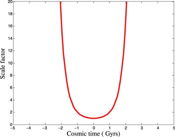
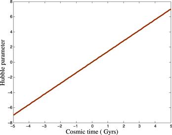
As singularity occurs during the expansion of the Universe, the inflationary scenario cannot provide a picture of the past history of the Universe. Therefore the matter bounce cosmology has been proposed, where the initial singularity can be avoided. In the initial phase of bouncing cosmology, matter dominates the Universe and then a bounce occurs without any singularity [39, 40]. In bouncing cosmology, the following are observed, (a) the scale factor decreases ($\dot{a}\lt 0$) in the contracting phase (negative time zone ), (b) the scale factor increases $\dot{a}\gt 0$ in the expanding phase (positive time zone), (c) at the matter bounce epoch (bouncing point), it yields $\dot{a}=0$. We have considered here a symmetric bounce, which can be described with the scale factor $a={{\rm{e}}}^{\gamma {t}^{2}}$, where γ is the positive constant parameter. It can be observed that the constant parameter γ has a major role in the cosmic expansion description. Further, the proposed scale factor does not experience any kind of singularities because the scale factor, the Hubble parameter and its derivatives are finite. Subsequently the Hubble parameter can be obtained as H=2γt.

Figure 1 depicts the behavior of the bouncing scale factor as a function of cosmic time. It is seen that at the bouncing epoch t=0, the scale factor is symmetrical in nature. The value of parameter γ imparts the slope of the curves of the scale factor. From figure 1, it is observed that as the value of γ increases, so does the curvature of the plot. At t=0, the value of the scale factor is constant; however it does not vanish which enables the fact that there is a null value of the Hubble parameter at the bouncing epoch. For a specific realization of a bounce, with H<0, it represents a contracting Universe whereas in an expanding Universe, it yields H>0. Hence in continuation, it is concluded that at the bounce point, we must have H=0 and around it, we must have H>0. Figure 2 depicts the linear behavior of the Hubble parameter as a function of cosmic time. With regard to the bouncing model, the Hubble parameter evolves linearly from the contracting Universe towards the expanding Universe through H=0 at bounce.

Figure 1.

New window|Download| PPT slide
Figure 1.Bouncing scale factor w.r.t. cosmic time.

Figure 2.

New window|Download| PPT slide
Figure 2.Hubble parameter w.r.t. cosmic time.


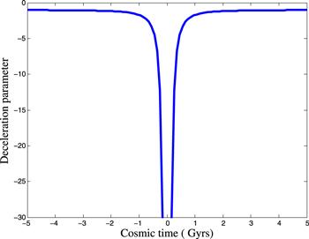
The deceleration parameter can be derived as, $q\,=-1-\tfrac{\dot{H}}{{H}^{2}}=-1-\tfrac{1}{2\gamma {t}^{2}}$. The rate of expansion of the Universe is measured with the help of the cosmological parameter known as deceleration parameter. The deceleration parameter signifies inflation if q<0 whereas for the positive value i.e. q>0, it represents decelerated Universe. The Universe shows expansion with a constant rate, if the value of the deceleration parameter exhibits q=0. At t=0 i.e. at bouncing point, the deceleration parameter shows symmetrical behavior. From figure 3, it is observed that for both the contracting and expanding universes, the deceleration parameter q is negative, and after some finite time it tends to a constant value −1. In the contacting Universe, the deceleration parameter tends to the large negative values at the bouncing point even after evolving from q=−1. In the positive frame of the cosmic time, the deceleration parameter tends to q=−1 at late times. Thus in the derived GRH model, the value of the deceleration parameter resembles with the recent cosmological observations of Type Ia Supernovae and the Universe is accelerating throughout the evolution [41-43].

Figure 3.

New window|Download| PPT slide
Figure 3.Deceleration parameter w.r.t. cosmic time.

4. Physical parameters

Now, with the bouncing scale factor and some algebraic manipulation, we can obtain from equations (8) and (9), the energy density ρ and pressure p of the defined GRH model as(10)$\begin{eqnarray}\rho =\displaystyle \frac{1}{1+{\rm{\Gamma }}\epsilon }\left[\displaystyle \frac{12(1+2\beta ){\gamma }^{2}{t}^{2}-4\beta \gamma }{{\alpha }^{2}-{\beta }^{2}}\right],\end{eqnarray}$(11)$\begin{eqnarray}p=-\left[\displaystyle \frac{12(1+2\beta ){\gamma }^{2}{t}^{2}+4\alpha \gamma }{{\alpha }^{2}-{\beta }^{2}}\right].\end{eqnarray}$

From equations (10) and (11), the pressure and energy density depend on the model parameter β and the scale factor γ, so the evolutionary behavior also depend on these two parameter. For γ=0.7, β=0.1, α=1.3, Γ=2, ε=0.8, the quantity α²−β²>0, which means that the denominators of the energy density and pressure are positive. Thus the positivity or the negativity of energy density and pressure depend only on the respective numerators. The energy density should remain positive, in order to satisfy certain energy conditions throughout the cosmic evolution. The energy density and pressure near the bouncing region decreases with the increment in the model parameter β. The choice of the value of the adiabatic index is purely based on the established experimental results [44, 45]. However, the profiles start to converge, away from the bouncing territory. The EoS parameter can be obtained as(12)$\begin{eqnarray}\omega =-(1+{\rm{\Gamma }}\epsilon )\left[\displaystyle \frac{12(1+2\beta ){\gamma }^{2}{t}^{2}+4\alpha \gamma }{12(1+2\beta ){\gamma }^{2}{t}^{2}-4\beta \gamma }\right].\end{eqnarray}$

To study the DE aspects of the model, three large class of scalar field DE models available in the literature such as the phantom ω<−1 [46], quintessence −1<ω≤0 [47] and the quintom ω cross −1. The quintom scenario can cross from phantom to quintessence region. As the EoS parameter is time dependent, The EoS parameter allows the model to transit from ω>−1 to ω<−1 [48]. Several observations suggest the limit for ω as (i) Supernovae cosmology project, $-{1.035}_{-0.059}^{+0.055}$ [49] (ii) WMAP+SN Ia, −1.084±0.063 [50], (iii) Planck collaboration, −1.03±0.03 [51].

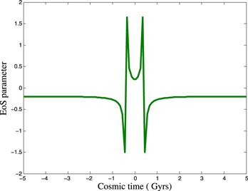
The EoS parameter is graphically represented in figure 4, which is time dependent. For β→0 , the corresponding GRH model reproduces the results of general relativity i.e. ${\omega }_{\beta \to 0}\left(1+\tfrac{1}{3\gamma {t}^{2}}\right)$. From figure 4 , it is observed that, the EoS parameter shows symmetrical behavior about the bouncing time t=0. From figure 4, it is clear that EoS parameter crosses −1 in the interval (0.4,0.5) in the time zone of both the contracting and expanding universes. Therefore, this particular phenomenological model of Universe is quintom model [52]. In the neighborhood of bouncing point, the EoS parameter undergoes phase transition from ω>−1 to ω<−1. So the model presented here favors the quintom model. Also, after the bounce, the Universe enters into hot big bang age [53].

Figure 4.

New window|Download| PPT slide
Figure 4.EoS parameter w.r.t. cosmic time.


In the negative time zone (contracting Universe), the EoS parameter evolves in the matter dominated Universe at the bouncing point from a large positive values and approaches the Quintessence region. In the positive time zone (expanding Universe), it evolves in a matter dominated Universe at the bouncing point, converges to large negative values and approaches the Quintessence region at late times. The evolving of the EoS parameter is rapid near the bounce as compared to the far away time frame. The concerned raise in the rate of increment of the EoS parameter near the bounce depends on the value of the scale factor parameter γ as shown in the figure 4. Away from the bounce, the parameter γ does not have any significant impact on the EoS parameter. The recent Pantheon analysis that combines SNeIa data from several surveys, obtained in ω_λ=−1.026±0.041 [54] and for a flat CDM model after combining with CMB constraints it becomes ω_λ=−0.978±0.059. The constraints of EoS parameter coincide with the Planck collaboration [55] and WMAP [50] which give the ranges for EoS parameter as (i) −0.92<ω<−1.26 (Planck + WP + Union 2.1), (ii) −0.89<ω<−1.38 (Planck+ WP +BAO), and (iii) −0.983<ω<−1.162 (WMAP+ eCMB+ BAO+ H₀). It can also be observed that the behavior of the model obtained, here, is in good agreement with the recent observational data.

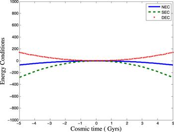
Energy conditions are mathematically imposed boundary conditions in an attempt to claim the positive energy. Many energy conditions related to physical situation, the most common example is, the effect of DE that violates the strong energy condition (SEC). The energy conditions describe the properties common to all the states of matter and all non-gravitational fields. It rules out the unphysical solutions to Einstein’s field equations. Four types of energy conditions are (i) null energy condition (NEC), ρ+p≥0; (ii) SEC, ρ+3p≥0; (iii) Dominant energy condition, ρ≥∣p∣; and (iv) Weak energy condition (WEC), ρ≥0. At the bouncing point, it is observed that H=0 and $\dot{H}\gt 0$. Also from figure 5, it is observed that ρ+p<0 and ρ+3p<0. Hence in this particular bouncing model, NEC and SEC both are violated as shown in figure 5. NEC and SEC are in the negative domain near the bounce point in both expanding and contracting Universe. Hence, as the energy conditions are violating, the model evolves in the phantom phase with both at ω<−1 and ω>−1.

Figure 5.

New window|Download| PPT slide
Figure 5.Energy conditions w.r.t. cosmic time.

5. Stability factor

The stability of the model is studied in literature by using the ratio of sound speed given by ${C}_{s}^{2}=\tfrac{{\rm{d}}p}{{\rm{d}}\rho }$. If ${C}_{s}^{2}\gt 0$, then the model is stable and for ${C}_{s}^{2}\lt 0$, the model is unstable. The stability factor in the derived model is given by(13)$\begin{eqnarray}{C}_{s}^{2}=-(1+{\rm{\Gamma }}\epsilon ).\end{eqnarray}$

Since Γ>0,ε>0, equation (13) gives ${C}_{s}^{2}\lt 0$. Hence from the stability point of view, the derived GRH model is unstable.

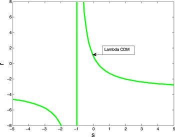
The state finder diagnostic pair (r,s), where r is the jerk parameter and s characterizes the property of DE need to be assessed since they involve the third derivative of the scale factor [56]. The numeric value of this pair leads to certain situations such as (i) when (r,s)=(1,0), it leads to ΛCDM model (ii) When (r,s)=(1,1), it leads to CDM limit, (iii) when r<1, it is quintessence DE region, and (iv) when s>0 phantom DE regions. The pair can be obtained as

$r=\tfrac{\dddot{a}}{{{aH}}^{3}}=1+\tfrac{3}{2\gamma {t}^{2}}$ and$s=\tfrac{r-1}{3\left(q-\tfrac{1}{2}\right)}=-\tfrac{1}{1\,+\,3\gamma {t}^{2}}$.

The relation between the state finder parameters can be obtained as, $r=1-\tfrac{9s}{2(1+s)}$. Figure 6 depicts the plot of r versus s. It can be observed that the state finder curve passes through the point (1,0), which means that the derived GRH model behaves as ΛCDM model during the evolution of the Universe. The two domain in the plot (r<1,s>0) and (r>1,s<0) leads to quintessence region and Chaplygin gas region respectively. The value of the state finder pair in the present epoch is obtained as (1.011, −0.0024).

Figure 6.

New window|Download| PPT slide
Figure 6.r versus s.


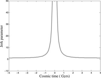
In cosmology, the third derivative of the scale factor with respect to the cosmic time is termed the jerk parameter [57]. It is defined as $j(t)=1+\tfrac{3}{2\gamma {t}^{2}}$. The model close to ΛCDM are discussed with the help of jerk parameter in cosmology. The negative value of the deceleration and positive value of the jerk parameter are responsible for the phase transition from deceleration to acceleration. The jerk parameter for the ΛCDM model has a constant jerk. The jerk parameter is represented graphically in figure 7. The jerk parameter depends on the scale factor parameter γ. At the bouncing epoch, the jerk parameter has a singular value because of the vanishing nature of the Hubble rate at bounce. At a large cosmic time away from the bounce, the jerk parameter decreases to small values close to one, which was outlined in our earlier work [58, 59].

Figure 7.

New window|Download| PPT slide
Figure 7.Jerk parameter w.r.t. cosmic time.

6. Discussion, concluding remarks and scope for future research

We have presented a matter bounce scenario in the presence of GRH in the framework of extended gravity. We have considered the bouncing scale factor in order to study the matter bounce scenario which provides a symmetric behavior around the bounce. The scale factor shows the decreasing behavior and after the bounce it increases again with respect to the cosmic time. In the present bouncing scenario, it yields a→∞ and a→∞ as t→∞. It shows that the possibility of finite-time singularities do not occur in this model. In the flat FRW Universe, at the bouncing point energy density remains positive but SEC is violated. Also, as the Universe is accelerating after the bounce, it has ρ+3p<0. The Universe accelerates with the negative value of the deceleration parameter, which is consistent with the present day observational results. Since the EoS parameter of the matter undergoes a phase transition from −1 to +1 near the bouncing point, the presented GRH model in extended gravity is referred as a quintom model. It is worthy to mention here that as compared to [30], in this work it has been observed that there is a marginal change in the dynamical behavior of the model with the inclusion of GRH in the matter part. Moreover the stability analysis indicates the instability of the model. This might be due to the inclusion of GRH. However in this scenario, the Universe still enters into the hot big bang age after the bounce. The behavior near the bounce is least affected by the bouncing scale factor; however it is mostly decided by the coupling parameter induced in the action of the extended gravity. It is important to study the GRH cosmological models with some other form of bouncing scale factors such as, hyperbolic function and power function, to understand the role of GRH in the expanding Universe.

Acknowledgments

BM acknowledges IUCAA, Pune, India for hospitality and support during an academic visit where a part of this work was accomplished. The authors are thankful to the anonymous referees for the valuable suggestions and comments for the improvement of the paper.

Reference View Option By original order
By published year
By cited within times
By Impact factor

[1]Riess A G et al. 1998 Astron. J. 116 1009
DOI:10.1086/300499 [Cited within: 1]

[2]Perlmutter S et al. 1999 Astrophys. J. 517 565
DOI:10.1086/307221 [Cited within: 1]

[3]de Bernadis P et al. 2000 Nature 404 955
DOI:10.1038/35010035 [Cited within: 1]

[4]Hanany S et al. 2000 Astrophys. J. 545 L5
DOI:10.1086/317322 [Cited within: 1]

[5]Contaldi A R Hoekstra H Lewis A 2003 Phys. Rev. Lett. 90 221303
DOI:10.1103/PhysRevLett.90.221303 [Cited within: 1]

[6]Tegmark M et al. 2004 Phys. Rev. D 69 103501
DOI:10.1103/PhysRevD.69.103501 [Cited within: 1]

[7]Cole S et al. 2005 Mon. Not. R. Astron. Soc. 362 505
DOI:10.1111/j.1365-2966.2005.09318.x

[8]Springel V et al. 2006 Nature 440 1137
DOI:10.1038/nature04805 [Cited within: 1]

[9]Spergel A N et al. 2007 Astrophys. J. Suppl. 170 377
DOI:10.1086/513700 [Cited within: 1]

[10]Ade P A R et al. 2016 Astron. Astrophys. 594 A13
DOI:10.1051/0004-6361/201525830 [Cited within: 1]

[11]Novello M Perez Bergliaffa S E 2008 Phys. Rep. 463 127
DOI:10.1016/j.physrep.2008.04.006 [Cited within: 1]

[12]Solomans D Dunsby P K S Ellis G F R 2006 Class. Quantum Grav. 23 6585 6597
DOI:10.1088/0264-9381/23/23/001 [Cited within: 1]

[13]Bamba K Makarenko A N 2014 J. Cosmol. Astropart. Phys. 01 008
DOI:10.1088/1475-7516/2014/01/008 [Cited within: 1]

[14]Silva G F et al. 2013 Gravit. Cosmol. 19 156
DOI:10.1134/S0202289313030109 [Cited within: 1]

[15]Sadatian S D 2014 Int. J. Theor. Phys. 53 675
DOI:10.1007/s10773-013-1855-1 [Cited within: 1]

[16]Astashenok A V 2014 Astrophys. Space Sci. 351 377
DOI:10.1007/s10509-014-1846-6 [Cited within: 1]

[17]Brevik I Obukhov V V Timoshkin A V 2014 Mod. Phys. Lett. A 29 1450078
DOI:10.1142/S0217732314500783 [Cited within: 1]

[18]Brevik I Obukhov V V Timoshkin A V 2014 Universe 1 24
DOI:10.3390/universe1010024 [Cited within: 1]

[19]Cai Y F et al. 2011 Class. Quantum Grav. 28 215011
DOI:10.1088/0264-9381/28/21/215011 [Cited within: 1]

[20]Cai Y F et al. 2012 J. Cosmol. Astropart. Phys. JCAP08(2012)20
DOI:10.1088/1475-7516/2012/08/020

[21]Cai Y F 2014 Sci. China Phys. Mech. Astron. 57 1414
DOI:10.1007/s11433-014-5512-3

[22]Cai Y F Wilson-Ewing E 2015 J. Cosmol. Astropart. Phys. JCAP03(2015)006
DOI:10.1088/1475-7516/2015/03/006 [Cited within: 1]

[23]Cai Y F et al. 2016 Universe 3 1
DOI:10.3390/universe3010001 [Cited within: 1]

[24]Brandenberger R Peter P 2017 Found. Phys. 47 797
DOI:10.1007/s10701-016-0057-0 [Cited within: 1]

[25]Bamba K et al. 2014 Phys. Lett. B 732 349
DOI:10.1016/j.physletb.2014.04.004 [Cited within: 1]

[26]Bamba K et al. 2015 J. Cosmol. Astropart. Phys. JCAP04(2015)01
DOI:10.1088/1475-7516/2015/04/001

[27]Bamba K et al. 2016 Phys. Rev. D 94 083513
DOI:10.1103/PhysRevD.94.083513 [Cited within: 1]

[28]de la Cruz-Dombriz A et al. 2018 Phys. Rev. D 97 104040
DOI:10.1103/PhysRevD.97.104040 [Cited within: 1]

[29]Minas G et al. 2019 Universe 5 74
DOI:10.3390/universe5030074 [Cited within: 1]

[30]Tripathy S K et al. 2019 Eur. Phys. J. Plus 134 504
DOI:10.1140/epjp/i2019-12879-3 [Cited within: 2]

[31]Tripathy S K Mishra B 2002arXiv:2002.03787v1
[Cited within: 1]

[32]Taub A H 1978 Ann. Rev. Fluid Mech. 10 301
DOI:10.1146/annurev.fl.10.010178.001505 [Cited within: 1]

[33]Font J A 2007 J. Phys.: Conf. Ser. 91 012002
DOI:10.1088/1742-6596/91/1/012002 [Cited within: 1]

[34]Font J A 2008 Living Rev. Relativ. 11 3
DOI:10.12942/lrr-2008-7 [Cited within: 1]

[35]Liptai D Price D J 2019 Mon. Not. R. Astron. Soc. 485 819
DOI:10.1093/mnras/stz111 [Cited within: 1]

[36]Kovtun P 2019 J. High Energy Phys. JHEP 1910 034
DOI:10.1007/JHEP10(2019)034 [Cited within: 1]

[37]Ananda K N Bruni M 2006 Phys. Rev. D 74 023523
DOI:10.1103/PhysRevD.74.023523 [Cited within: 1]

[38]Singh A et al. 2018 Int. J. Mod. Phys. A 33 1850213
DOI:10.1142/S0217751X18502135 [Cited within: 1]

[39]Tripathy S K et al. 2020 Int. J. Geom. Methods Mod. Phys. 17 2050056
DOI:10.1142/S0219887820500565 [Cited within: 1]

[40]Molina-Paris C Visser M 1999 Phys. Lett. B 455 90
DOI:10.1016/S0370-2693(99)00469-4 [Cited within: 1]

[41]Torny J L et al. 2003 Astrophys. J. 594 1
DOI:10.1086/376865 [Cited within: 1]

[42]Reiss A G et al. 2004 Astron. J. 607 665
DOI:10.1086/383612

[43]Clocchiatti A et al. 2006 Astrophys. J. 642 1
DOI:10.1086/498491 [Cited within: 1]

[44]Baiotti L Giacomazzo B Rezzolla L 2008 Phys. Rev. D 78 084033
DOI:10.1103/PhysRevD.78.084033 [Cited within: 1]

[45]Montero P J Baumgarte T W Muller E 2014 Phys Rev. D 89 084043
DOI:10.1103/PhysRevD.89.084043 [Cited within: 1]

[46]Caldwell R 2002 Phys. Lett. B 545 23
DOI:10.1016/S0370-2693(02)02589-3 [Cited within: 1]

[47]Steinhardt P Wang L Zlatev I 1999 Phys. Rev. D 59 123504
DOI:10.1103/PhysRevD.59.123504 [Cited within: 1]

[48]Wang B Gong Y Abdalla E 2006 Phys. Rev. D 74 083520
DOI:10.1103/PhysRevD.74.083520 [Cited within: 1]

[49]Amanullah R et al. 2010 Astrophy. J. 716 712
DOI:10.1088/0004-637X/716/1/712 [Cited within: 1]

[50]Hinshaw G et al. 2013 Astrophys. J. Suppl. Ser. 208 19
DOI:10.1088/0067-0049/208/2/19 [Cited within: 2]

[51]Aghanim N(Planck Collaboration)et al. 2020 Astron. Astrophys. 641 A6
DOI:10.1051/0004-6361/201833910 [Cited within: 1]

[52]Feng B Wang X Zhang X 2005 Phys. Lett. B 607 35
DOI:10.1016/j.physletb.2004.12.071 [Cited within: 1]

[53]Cai Y F et al. 2007 J. High Energy Phys. JHEP10(2007)071
DOI:10.1088/1126-6708/2007/10/071 [Cited within: 1]

[54]Scolnic D M et al. 2018 Astrophys J. 859 101
DOI:10.3847/1538-4357/aab9bb [Cited within: 1]

[55]Ade P A R et al. 2014 Astron. Astrophys. 571 A16
DOI:10.1051/0004-6361/201321591 [Cited within: 1]

[56]Sahni V et al. 2003 J. Exp. Theor. Phys. 77 201
[Cited within: 1]

[57]Chiba T Nakamura T 1998 Prog. Theor. Phys. 100 1077
DOI:10.1143/PTP.100.1077 [Cited within: 1]

[58]Shaikh A Y et al. 2019 J. Astrophys. Astron. 40 25
DOI:10.1007/s12036-019-9591-4 [Cited within: 1]

[59]Shaikh A Y Gore S V Katore S D 2020 New Astron. 80 101420
DOI:10.1016/j.newast.2020.101420 [Cited within: 1]