Aisha Siddiqa^,Department of Mathematics, Virtual University of Pakistan, 54-Lawrence Road, Lahore, Pakistan

Received:2019-10-11Revised:2019-12-22Accepted:2019-12-24Online:2020-02-24


Abstract
This paper presents a picture of compact structures for the f(R, T) model of the form R+γ e^χT, with γ and χ being parameters. The polytropic equation of state and the MIT bag model reflect the pressure density relation for these compact objects. For this purpose, a system of two differential equations involving pressure as well as the mass of the stellar structure is obtained from field equations and the Tolman–Oppenheimer–Volkoff (TOV) equation. The numerical solution of this system gives a graphical description of various characteristics of these compact systems. To examine the viability and stability of assumed configurations, the energy conditions, causality relation and adiabatic index are discussed for the presumed scenario.
Keywords： f(R, T) gravity;neutron and quark stars;equation of state


PDF (478KB)MetadataMetricsRelated articlesExportEndNote|Ris|BibtexFavorite
Cite this article
Aisha Siddiqa. A view of compact configurations from the R+γe^χT scenario. Communications in Theoretical Physics, 2020, 72(3): 035402- doi:10.1088/1572-9494/ab690a

1. Introduction

Compact stellar remnants after the explosion of massive stars are white dwarfs, neutron stars, black holes and supermassive black holes. The formation of these compact structures depends upon the primary mass of the star. Each of these objects is a subject of great interest with its own fascinating physical features. These objects are not just hypothetical terms; they also exist in our universe. The existence of white dwarfs and neutron stars in our universe is supported by many observational evidence [1]. However, the existence of black holes is strongly reinforced by the discovery of gravitational waves and the recently captured image of a black hole by radio telescopes.

General relativity (GR) provides a rostrum to discuss different astrophysical and cosmological phenomena. However, from the last two decades, after the discovery of accelerated expansion of the Universe, different modifications of GR are proposed by researchers to cope with this issue. One of them is the f(R, T) theory of gravity proposed by Harko et al [2], where R and T correspond to the Ricci scalar and trace of stress energy tensor. This coupling introduces extra terms in the field equation that can mimic the source of accelerated expansion, produce a deviation from geodesic motion as well as assist in the study of the dark matter–dark energy interactions [3]. Several issues, such as cosmic evolution [4–8], thermodynamic laws [9–12] and wormhole configurations [13–16], have been investigated in this context.

The study of gravitational collapse and its leftovers has been extensively accomplished in GR and its extensions. Here, we elaborate on some of them regarding the stability of compact objects in modified theories. Abbas and Sarwar [17] examined expansion-free systems for stability in Einstein Gauss–Bonnet gravity with the conclusions that the system is stable only for chosen parametric values. Noureen and Zubair [18] investigated the stability of a spherical star with anisotropic fluid in f(R, T) gravity and obtained some limitations for physical quantities. Zubair and Abbas [19] considered three observed models of compact configurations and investigated their stability as well as viability in f(R) gravity assuming the Krori and Barua solution. Moraes et al [20] examined the equilibrium structure of neutron stars for the polytropic equation of state (EoS) and quark stars for the bag model concluding that the extreme mass can cross observational limits.

Deb et al [21] explored some features for strange stars assuming a decreasing density profile in the framework of f(R, T) gravity. Yousaf et al [22] explored the issue of stability for cylindrical stellar models via a perturbation technique finding that it relies on the stiffness parameter, matter variables and higher order curvature terms of the f(R, T) theory. Sharif and Siddiqa [23] studied the stability of compact objects via different models, fluid distributions and EoS. Astashenok et al [24] analyzed the existence of realistic stellar configurations for the f(R)=R+α R² gravity model. Carvalho et al [25] explored white dwarfs in f(R, T) theory finding that mass can violate the Chandrasekhar limit. Sharif and Waseem [26] investigated the stability of particular quark star models with anisotropic fluid in f(R, T) gravity using Krori and Barua ansatz.

Recently, Moraes and Sahoo [27] proposed a new functional form for f(R, T) as R+γ e^χT. They showed that the energy conditions are satisfied for wormhole solutions in this context. Moraes et al [28] examined the viability of this model in cosmic evolution. They derived different cosmic parameters and found satisfactory results by comparing them with observational data. This article is devoted to the investigation of the structure of compact stars for this model. The scheme of the paper is mentioned here. In the coming section, equations of stellar structure are formulated for f(R, T)=R+γe^χT. Section 3 elaborates the formation of compact stars and the assumed EoS for their matter. Section 4 gives the analysis of physical features for such compact stars for this model, and the last section summarizes and concludes the manuscript.

2. Stellar structure formalism

This study deals with a spherical symmetric stellar object whose geometry is described with the following spacetime(1)$\begin{eqnarray}\begin{array}{rcl}{{\rm{d}}s}^{2} & = & -{A}_{1}(r){{\rm{d}}t}^{2}+{A}_{2}(r){{\rm{d}}r}^{2}\\ & & +\,{r}^{2}({\rm{d}}{\theta }^{2}+{\sin }^{2}\theta {\rm{d}}{\phi }^{2}),\end{array}\end{eqnarray}$and stellar fluid distribution is defined by the following stress energy tensor(2)$\begin{eqnarray}\varepsilon {T}_{\beta \delta }=(\varepsilon +p){V}_{\beta }{V}_{\delta }+{{pg}}_{\beta \delta },\end{eqnarray}$where ${V}_{\beta }$, ϵ and p are fluid’s four velocity, energy density and pressure, respectively. Also, the trace of stress energy tensor is $T=-\varepsilon +3p$.

The modified Einstein–Hilbert action for curvature-matter coupling is given by(3)$\begin{eqnarray}S=\int \left[\displaystyle \frac{1}{16\pi }f(R,T)+{{ \mathcal L }}_{m}\right]\sqrt{-g}{{\rm{d}}}^{4}x,\end{eqnarray}$and the Einstein field equations are(4)$\begin{eqnarray}\begin{array}{l}{f}_{R}{R}_{\beta \delta }-\displaystyle \frac{1}{2}{g}_{\beta \delta }f+({g}_{\beta \delta }\square -{{\rm{\nabla }}}_{\beta }{{\rm{\nabla }}}_{\delta }){f}_{R}\\ \qquad =\,8\pi {T}_{\beta \delta }-{f}_{T}({T}_{\beta \delta }+{{\rm{\Theta }}}_{\beta \delta }),\end{array}\end{eqnarray}$where Θ_βδ has the following expression(5)$\begin{eqnarray}{{\rm{\Theta }}}_{\beta \delta }={g}^{\gamma \sigma }\displaystyle \frac{\delta {T}_{\gamma \sigma }}{\delta {g}^{\beta \delta }},\quad {T}_{\beta \delta }={g}_{\beta \delta }{{ \mathcal L }}_{m}-\displaystyle \frac{\partial {{ \mathcal L }}_{m}}{\partial {g}^{\beta \delta }}.\end{eqnarray}$Here, it is assumed that ${{ \mathcal L }}_{m}=p$ and the gravity model f(R, T)=R+γ e^{χ T} (with the dimensions of γ and χ as L⁻²) such that equation (4) is reduced to(6)$\begin{eqnarray}{G}_{\beta \delta }=8\pi {T}_{\beta \delta }+\displaystyle \frac{1}{2}{g}_{\beta \delta }\gamma {{\rm{e}}}^{\chi T}-{f}_{T}({g}_{\beta \delta }P-{T}_{\beta \delta }).\end{eqnarray}$The field equations for equation (1) are obtained as(7)$\begin{eqnarray}\begin{array}{l}\displaystyle \frac{{A}_{2}^{\prime} }{{{rA}}_{2}^{2}}+\displaystyle \frac{1}{{r}^{2}}-\displaystyle \frac{1}{{r}^{2}{A}_{2}}=8\pi \varepsilon \\ \,+\,\gamma {{\rm{e}}}^{\chi \left(3p-\varepsilon \right)}\left[-\displaystyle \frac{1}{2}+\chi (\varepsilon +p)\right],\end{array}\end{eqnarray}$(8)$\begin{eqnarray}\displaystyle \frac{{A}_{1}^{\prime} }{{{rA}}_{2}{A}_{1}}-\displaystyle \frac{1}{{r}^{2}}+\displaystyle \frac{1}{{r}^{2}{A}_{2}}=8\pi p+\displaystyle \frac{\gamma }{2}{{\rm{e}}}^{\chi 3p-\varepsilon }.\end{eqnarray}$

The mass of the stellar sphere with radius r is defined as $m=\tfrac{r}{2}\left(1-\tfrac{1}{{A}_{2}}\right)$, and using field equations its derivative has the expression(9)$\begin{eqnarray}m^{\prime} =4\pi {r}^{2}\varepsilon +\displaystyle \frac{\gamma }{2}{r}^{2}{{\rm{e}}}^{\chi (\varepsilon +p)}\left[\displaystyle \frac{-1}{2}+\chi (\varepsilon +p)\right].\end{eqnarray}$

The covariant derivative of the energy-momentum tensor is obtained as [29]$\begin{eqnarray*}\begin{array}{rcl}{{\rm{\nabla }}}^{\beta }{T}_{\beta \delta } & = & \displaystyle \frac{{f}_{T}}{8\pi -{f}_{T}}\left[[,,({T}_{\beta \delta }+{{\rm{\Theta }}}_{\beta \delta }){{\rm{\nabla }}}^{\beta }\mathrm{ln}{f}_{T}\right.\\ & & \left.+\,{{\rm{\nabla }}}^{\beta }{{\rm{\Theta }}}_{\beta \delta }-\displaystyle \frac{1}{2}{g}_{\beta \delta }{{\rm{\nabla }}}^{\beta }T\right],\end{array}\end{eqnarray*}$and for f(R, T)=R+γ e^{χ T}, it gives$\begin{eqnarray*}{{\rm{\nabla }}}^{\beta }{T}_{\beta \delta }=\displaystyle \frac{\gamma \chi {{\rm{e}}}^{\chi T}}{8\pi -\gamma \chi {{\rm{e}}}^{\chi T}}\left[{{\rm{\nabla }}}^{\beta }{{\rm{\Theta }}}_{\beta \delta }-\displaystyle \frac{1}{2}{g}_{\beta \delta }{{\rm{\nabla }}}^{\beta }T\right].\end{eqnarray*}$The corresponding Tolman–Oppenheimer–Volkoff equation, or TOV equation, is obtained after simplification as$\begin{eqnarray*}p^{\prime} +(\varepsilon +p)\displaystyle \frac{{A}_{1}^{{\prime} }}{2{A}_{1}}=\displaystyle \frac{\gamma \chi {{\rm{e}}}^{\chi T}}{2(8\pi -\gamma \chi {{\rm{e}}}^{\chi T})}(\varepsilon ^{\prime} -p^{\prime} ).\end{eqnarray*}$Substituting the value of $\tfrac{{A}_{1}^{{\prime} }}{{A}_{1}}$ from equation (8), it becomes(10)$\begin{eqnarray}p^{\prime} =-\displaystyle \frac{(\varepsilon +p)\left(8\pi {pr}+\tfrac{\gamma }{2}{{re}}^{\chi 3p-\varepsilon }+\tfrac{2m}{{r}^{2}}\right)}{\left(1-\tfrac{2m}{r}\right)\left[1+\tfrac{\gamma \chi {{\rm{e}}}^{\chi 3p-\varepsilon }}{2(8\pi -\gamma \chi {{\rm{e}}}^{\chi 3p-\varepsilon })}\left(1-\tfrac{{\rm{d}}\varepsilon }{{\rm{d}}{p}}\right)\right]}.\end{eqnarray}$

In the onward discussion, equations (9) and (10) are considered, which are in terms of density, pressure and the mass of a stellar configuration. To reduce one variable, the relation between pressure and density is incorporated via the EoS.

3. Compact objects and their EoS

In ordinary stars, fusion processes convert hydrogen into helium providing the thermal pressure to counterbalance gravity. With the running time, the helium reservoir in the core of a star is fused into heavier elements like carbon and oxygen. Consequently, the nuclear processes stop, the temperature is decreased and the pressure is increased in the core of the star. When the primary mass of the star is less than eight times the solar mass, the carbon fusion cannot take place and, after blowing the outer layers, the star ends up with a compact stage called a white dwarf. In white dwarfs, the electron degeneracy pressure (based on the Pauli exclusion principle) provides the counter force to gravity. Electrons are the first particles to degenerate, and the role of nuclei pressure is negligible here.

However, if the primary mass of the star is more than eight times the solar mass a larger degeneracy pressure or greater density is required to balance gravitational pull. This pressure originates from the neutron degeneracy pressure which is formed by protons and electrons. The resulting object is in hydrostatic equilibrium and is named a neutron star. Neutron stars are smaller and denser than white dwarfs. The temperature of white dwarfs and neutron stars is very low and tends to zero as time passes. Considering ideal circumstances where the compact object is composed of a single non-interacting fermion species at null temperature the EoS has the polytropic form p=ωϵ^κ; here, ω and κ correspond to the polytropic constant and index, respectively. Here, it is assumed that the compact structure has the EoS $p=\omega {\varepsilon }^{\tfrac{5}{3}}$, where the index $\kappa =\tfrac{5}{3}$ represents the fact that fluid particles are non-relativistic. Substituting the polytropic EoS in equations (9) and (10), the following system of two ordinary non-linear differential equations is obtained in terms of stellar pressure and mass(11)$\begin{eqnarray}\begin{array}{rcl}m^{\prime} & = & 4\pi {r}^{2}({\left(\displaystyle \frac{p}{\omega }\right)}^{\tfrac{3}{5}}+\displaystyle \frac{\gamma }{2}{r}^{2}{{\rm{e}}}^{\chi \left({\left(\tfrac{p}{\omega }\right)}^{\tfrac{3}{5}}+p\right)}\\ & & \times \,\left[\displaystyle \frac{-1}{2}+\chi \left({\left(\displaystyle \frac{p}{\omega }\right)}^{\tfrac{3}{5}}+p\right)\right],\end{array}\end{eqnarray}$(12)$\begin{eqnarray}p^{\prime} =-\displaystyle \frac{\left({\left(\tfrac{p}{\omega }\right)}^{\tfrac{3}{5}}+p\right)\left(8\pi {pr}+\tfrac{\gamma }{2}{{r}{\rm{e}}}^{\chi T}+\tfrac{2m}{{r}^{2}}\right)}{\left(1-\tfrac{2m}{r}\right)\left[1+\tfrac{\gamma \chi {{\rm{e}}}^{\chi T}}{2\left(8\pi -\gamma \chi {{\rm{e}}}^{\chi 3p-\varepsilon }\right)}\left(1-\tfrac{3}{5\omega }{\left(\tfrac{p}{\omega }\right)}^{-\tfrac{2}{5}}\right)\right]}.\end{eqnarray}$

For graphical analysis, as well as to relate the compact structure to realistic stellar models, the value of ω is taken as ω≃0.000 5 (fm³/MeV)^2/3 [30], which is obtained for neutron stars, and the central pressure is taken as p₀≃220MeV/fm³, which is for the heaviest stable neutron star [31]. To solve the above defined systems numerically, the following initial conditions are assumed$\begin{eqnarray*}m(0)=0\quad P(0)=220\,\mathrm{MeV}/{\mathrm{fm}}^{3}.\end{eqnarray*}$Here, the units are taken as: km for radius, M_⊙ for mass and MeV/fm³ for density and pressure [20].

At certain densities and below, the matter of compact objects may be composed of protons, electrons, neutrons, positrons, neutrinos and antineutrinos. However, in denser matter the constituents may also include muons, hyperons and quarks [30]. If the stellar matter is composed of quarks then the corresponding compact object is called a quark star. The formation of quark stars from neutron stars has been discussed in the literature [32]. Different approaches used to obtain a satisfactory EoS for quark matter showed that quarks should be supposed to be confined within some region termed as a bag. In this respect, the frequently used model is the MIT bag model proposed by scientists from MIT [33]. The EoS for this model is p=a(ϵ−4b), where a and b are constants.

For the MIT bag model, the structure equations (9) and (10) take the following form(13)$\begin{eqnarray}\begin{array}{rcl}m^{\prime} & = & 4\pi {r}^{2}\left(\displaystyle \frac{p}{a}+4b\right)+\displaystyle \frac{\gamma }{2}{r}^{2}{{\rm{e}}}^{\chi \left(\left(\tfrac{p}{a}+4b\right)+p\right)}\\ & & \times \,\left[\displaystyle \frac{-1}{2}+\chi \left(\left(\displaystyle \frac{p}{a}+4b\right)+p\right)\right],\end{array}\end{eqnarray}$(14)$\begin{eqnarray}p^{\prime} =-\displaystyle \frac{\left(\left(\tfrac{p}{a}+4b\right)+p\right)\left(8\pi {pr}+\tfrac{\gamma }{2}{{r}{\rm{e}}}^{\chi T}+\tfrac{2m}{{r}^{2}}\right)}{\left(1-\tfrac{2m}{r}\right)\left[1+\tfrac{\gamma \chi {{\rm{e}}}^{\chi T}}{2\left(8\pi -\gamma \chi {{\rm{e}}}^{\chi 3p-\varepsilon }\right)}\left(1-\tfrac{1}{a}\right)\right]}.\end{eqnarray}$

Here, the quark star is considered to be composed of the lightest quarks that are up, down and strange quarks. In the literature, the constant a has the value a≃0.33 for such matter [20], while different values for the bag constant b are considered in the literature [20, 34]. In this manuscript, I consider $b=60{MeV}/{{fm}}^{3}$ and the following initial conditions for the quark star matter distribution$\begin{eqnarray*}m(0)=0\quad P(0)=500\,\mathrm{MeV}/{\mathrm{fm}}^{3}.\end{eqnarray*}$

4. Analysis of physical features

In this section, the numerical analysis of physical characteristics is given for the compact structures obeying the polytropic EoS and MIT bag relation. For convenience, all the plots for the polytropic case are presented in a red color and for the MIT bag model they are in a purple color. For a smooth interpretation, these characteristics are split up into the following subsections.

4.1. EoS variables

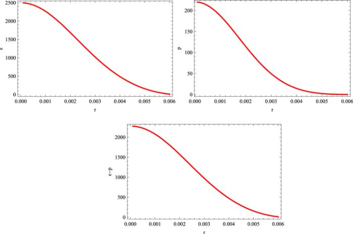
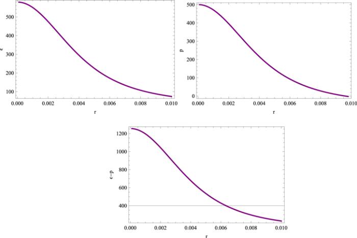
The term EoS variables corresponds to the density and pressure of the fluid configuration. Assuming the above-mentioned values of the parameters, as well as the initial conditions, the following graphs are obtained for EoS variables corresponding to the polytropic equation and MIT bag model. Also, the model parameters γ and χ are assumed to be unity, i.e. γ=1=χ.

The left graph of figure 1 gives the density profile, while the right one interprets the behavior of the pressure for the polytropic star. Both functions are positive and decreasing, and p(0.006)≃0 indicates that r≃0.006 km is the radius of the polytropic star in the considered scenario. Similarly, figure 2 explains the behavior of density and pressure for the quark star model in this background. For the assumed values of all parameters, the radius of the quark star is observed as r≃0.01 km.

Figure 1.

New window|Download| PPT slide
Figure 1.Density (ϵ), pressure (p) and their difference (ϵ-p) versus radial coordinate r for $p=0.000\,5{\varepsilon }^{\tfrac{5}{3}}$.

Figure 2.

New window|Download| PPT slide
Figure 2.Density (ϵ), pressure (p) and their difference (ϵ-p) versus radial coordinate r for p=0.33(ϵ−240).


In the study of stellar structures the discussion of energy conditions is necessary to exclude the possibility of un-realistic matter. Moreover, the energy conditions ensuring viability of the fluid configuration are: ϵ+p≥0 (NEC), ϵ≥0, ϵ+p≥0 (WEC), ϵ−p≥0 (DEC) and ϵ+3p≥0 (SEC). A sharp overview of the plots in figures 1 and 2 indicates that all the energy conditions are satisfied for both cases as ϵ≥0, p≥0 and ϵ−p≥0 for both cases.

4.1.1. Mass and Associated Quantities

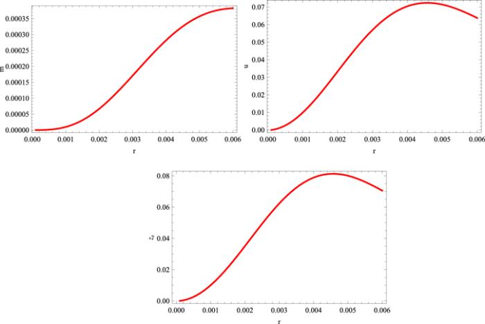
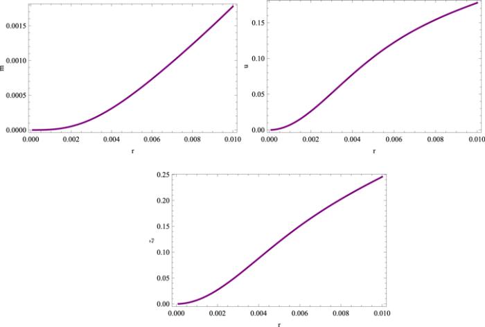
In the same pattern from the two sets of differential equations, the plots for the mass functions of the stellar configurations are obtained. The expressions for the compactness factor u(r) as well as the surface gravitational redshift z_s(r) in terms of mass function are given by(15)$\begin{eqnarray}u(r)=\displaystyle \frac{m(r)}{r},\end{eqnarray}$(16)$\begin{eqnarray}{z}_{s}(r)={\left(1-2\displaystyle \frac{m(r)}{r}\right)}^{-\tfrac{1}{2}}-1.\end{eqnarray}$

The graphical behavior of functions m(r), u(r) and z_s for the polytropic EoS are given in figure 3. The mass increases for all values of the radial coordinate, while the compactness and redshift first increase and after r≃0.004 5 decrease slightly. Similarly, figure 4 interprets the mass, compactness and redshift for the MIT bag model, which are all increasing with respect to the radial coordinate.

Figure 3.

New window|Download| PPT slide
Figure 3.Mass (m), compactness (u) and surface redshift (z_s (r)) versus radial coordinate r for $p=0.000\,5{\varepsilon }^{\tfrac{5}{3}}$.

Figure 4.

New window|Download| PPT slide
Figure 4.Mass (m), compactness (u) and surface redshift (z_s (r)) versus radial coordinate r for p=0.33(ϵ−240).

4.1.2. Stability Analysis

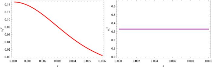
In general, the stability of the stellar structure corresponds to dynamical stability and thermal stability. Here, we do not consider thermal stability as the compact structures considered have very low temperature and cooling down with time. For stability analysis, the speed of sound profile is obtained for both EoS. If the speed of sound remains between zero and unity the causality relation holds for this fluid distribution. This condition also defines the stability criteria of the stellar configuration. The plots in figure 5 indicate that v_s lies between these limits yielding the stability of the polytropic star and quark star for the corresponding set of parameters and initial conditions.

Figure 5.

New window|Download| PPT slide
Figure 5.The speed of sound for $p=0.000\,5{\varepsilon }^{\tfrac{5}{3}}$ (left) and p=0.33(ϵ−240) (right).


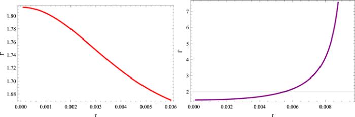
The stability of a stellar system can also be observed through the adiabatic index, denoted and defined as ${\rm{\Gamma }}=\tfrac{\epsilon +p}{p}\tfrac{{\rm{d}}{p}}{{\rm{d}}\epsilon }$. For a stable configuration, it should be greater than $\tfrac{4}{3}$ such that the system’s total energy remains bounded and, if the adiabatic index is less than $\tfrac{4}{3}$, then the energy becomes unbounded and ultimately the star explodes. Figure 6 gives the plots for both cases and, according to these, both configurations are stable.

Figure 6.

New window|Download| PPT slide
Figure 6.The adiabatic index for $p=0.000\,5{\varepsilon }^{\tfrac{5}{3}}$ (left) and p=0.33(ϵ−240) (right).

5. Summary and conclusions

This paper examined the physical properties of a compact stellar structure and their stability in the framework of an exponential model proposed in [27]. In this respect, the polytropic EoS and MIT bag model are considered to accommodate compact stars. The EoS parameters and initial conditions are chosen accordingly. The numerical solution of the structure equations for these chosen conditions and parameters depicts the physical features of compact objects.

In general, for a stellar structure, density as well as pressure are decreasing while the mass function is growing with the increment in the radial coordinate. Similar behavior of these functions is observed here, and the energy conditions are satisfied implying realistic matter distribution. The compactness and redshift measures fall within the bounds defined in the literature for perfect fluid [35], and the masses are below the well known Chandrasekhar [1] and TOV limits [36]. The change in the values of constants a and b in the MIT bag model are also observed, and it is found that the radius of the quark star grows with the increase in a while it decreases with the increment in b, which is compatible with [34].

In this study, the radii of stellar configurations that have a structure similar to neutron stars as well as quark stars are very small. This small radius can be associated with the effects of the f(R, T) gravity model in such a way that due to the exponential form of the model the corresponding change in physical characteristics is also rapid or exponential. Consequently, due to these small radii very large values of the model parameters induce a change in the physical properties of the star. The aim of this work is to explore the existence of stable stellar structures for such an exponential model, and it has been shown that stable configurations can exist in this scenario.

Neutron stars, being very small objects, are detectable and observable if they are pulsars (means rotating and emitting radiation) or if they are in a binary system. From an observational point of view thermal emission, explosions on the surface and gravitational wave emission from neutron stars are the sources for their mass and radius measurements. A huge number of neutron stars are expected to exist in our Universe as only the Milky Way is thought to contain 100 million neutron stars estimated by the number of supernova explosions. A gravitational wave signal has also been observed from the merger of two neutron stars [37]. However, the radii and masses of compact stars obtained in this manuscript are very small. This can be associated with the effects of the f(R, T) gravity model that due to the exponential form of coupling the change in physical characteristics is also rapid or exponential. It can be presumed that such small compact stars may exist among the family of such objects in our cosmos.

Reference View Option By original order
By published year
By cited within times
By Impact factor

[1]Shapiro S L Teukolsky S A 1983 Black Holes, White Dwarfs and Neutron Stars The Physics of Compact Objects New York Wiley
[Cited within: 2]

[2]Harko T Lobo F S N Nojiri S Odintsov S D 2011 Phys. Rev. D 84 024020
DOI:10.1103/PhysRevD.84.024020 [Cited within: 1]

[3]Harko T Lobo F S N 2014 Galaxies 2 410
DOI:10.3390/galaxies2030410 [Cited within: 1]

[4]Jamil Met al. 2012 Eur. Phys. J. C 72 1999
DOI:10.1140/epjc/s10052-012-1999-9 [Cited within: 1]

[5]Houndjo M J S 2012 Int. J. Mod. Phys. D 21 1250003
DOI:10.1142/S0218271812500034

[6]Sharif M Nawazish I 2017 Eur. Phys. J. C 77 198
DOI:10.1140/epjc/s10052-017-4773-1

[7]Sharif M Siddiqa A 2017 Mod. Phys. Lett. A 32 1750151
DOI:10.1142/S0217732317501516

[8]Sharif M Siddiqa A 2018 Commun. Theor. Phys. 69 537
DOI:10.1088/0253-6102/69/5/537 [Cited within: 1]

[9]Sharif M Zubair M 2012 J. Cosmol. Astropart. Phys. 03 028
DOI:10.1088/1475-7516/2012/03/028 [Cited within: 1]

[10]Jamil M Momeni D Myrzakulov R 2012 Chin. Phys. Lett. 29 109801
DOI:10.1088/0256-307X/29/10/109801

[11]Sharif M Zubair M 2013 Exp. Theor. Phys. 117 248
DOI:10.1134/S1063776113100075

[12]Momeni D Moraes P H R S Myrzakulov R 2016 Astrophys. Space Sci. 361 228
DOI:10.1007/s10509-016-2784-2 [Cited within: 1]

[13]Zubair M Waheed S Ahmad Y 2016 Eur. Phys. J. C 76 444
DOI:10.1140/epjc/s10052-016-4288-1 [Cited within: 1]

[14]Moraes P H R S Sahoo P K 2017 Phys. Rev. D 96 044038
DOI:10.1103/PhysRevD.96.044038

[15]Zubair M Mustafa G Waheed S Abbas G 2017 Eur. Phys. J. C 77 680
DOI:10.1140/epjc/s10052-017-5251-5

[16]Sahoo P K Moraes P H R S Sahoo P 2018 Eur. Phys. J. C 78 46
DOI:10.1140/epjc/s10052-018-5538-1 [Cited within: 1]

[17]Abbas G Sarwar S 2014 Astrophys. Space Sci. 352 769
DOI:10.1007/s10509-014-1992-x [Cited within: 1]

[18]Noureen I Zubair M 2015 Astrophys. Space Sci. 356 103
DOI:10.1007/s10509-014-2202-6 [Cited within: 1]

[19]Zubair M Abbas G 2016 Astrophys. Space Sci. 361 342
DOI:10.1007/s10509-016-2933-7 [Cited within: 1]

[20]Moraes P H R S José D V A Malheiro M 2016 J. Cosmol. Astropart. Phys. 06 005
DOI:10.1088/1475-7516/2016/06/005 [Cited within: 4]

[21]Deb D Rahaman F Ray S Guha B K 2018 J. Cosmol. Astropart. Phys. 03 044
DOI:10.1088/1475-7516/2018/03/044 [Cited within: 1]

[22]Yousaf Z Bhatti M Z Ume F 2017 Class. Quantum Grav. 34 145002
DOI:10.1088/1361-6382/aa73b9 [Cited within: 1]

[23]Sharif M Siddiqa A 2017 Eur. Phys. J. Plus 132 529
DOI:10.1140/epjp/i2017-11810-4 [Cited within: 1]

Sharif M Siddiqa A 2018 Phys. J. Plus 133 226
DOI:10.1140/epjp/i2017-11810-4 [Cited within: 1]

Sharif M Siddiqa A 2018 Int. J. Mod. Phys. D 27 1850065
DOI:10.1140/epjp/i2017-11810-4 [Cited within: 1]

[24]Astashenok A V de la Cruz-Dombriz A Odintsov S D 2017 Class. Quantum Grav. 34 205008
DOI:10.1088/1361-6382/aa8971 [Cited within: 1]

[25]Carvalho G Aet al. 2017 Eur. Phys. J. C 77 871
DOI:10.1140/epjc/s10052-017-5413-5 [Cited within: 1]

[26]Sharif M Waseem A 2018 Eur. Phys. J. C 78 868
DOI:10.1140/epjc/s10052-018-6363-2 [Cited within: 1]

[27]Moraes P H R S Sahoo P K 2019 Eur. Phys. J. C 79 677
DOI:10.1140/epjc/s10052-019-7206-5 [Cited within: 2]

[28]Moraes P H R S Sahoo P K Pacif S K J 2019(arXiv:1905.00417)
[Cited within: 1]

[29]Barrientos J Rubilar G F 2014 Phys. Rev. D 90 028501
DOI:10.1103/PhysRevD.90.028501 [Cited within: 1]

[30]Sagert I Hempel M Greiner C Bielich J S 2006 Eur. J. Phys. 27 577
DOI:10.1088/0143-0807/27/3/012 [Cited within: 2]

[31]Oppenheimer J R Volkoff G M 1939 Phys. Rev. 55 15
DOI:10.1103/PhysRev.55.374 [Cited within: 1]

[32]Haensel P Zdunik J L Schaeffer R 1986 Astron. Astrophys. 160 121
DOI:10.1103/PhysRevD.46.1274 [Cited within: 1]

Glendenning N K 1992 Phys. Rev. D 46 1274
DOI:10.1103/PhysRevD.46.1274 [Cited within: 1]

Lattimer J M Prakash M 2001 Astrophys. J. 550 426
DOI:10.1103/PhysRevD.46.1274 [Cited within: 1]

[33]Chodos A Jaffe B L Johnson K Thorn C B Weisskopf V F 1974 Phys. Rev. D 9 3471
DOI:10.1103/PhysRevD.9.3471 [Cited within: 1]

[34]Alaverdyan G B Vartanyan Y L 2017 Astrophysics 60 563
DOI:10.1007/s10511-017-9507-4 [Cited within: 2]

[35]Buchdahl H A 1959 Phys. Rev. 116 1027
DOI:10.1103/PhysRev.116.1027 [Cited within: 1]

[36]Bombaci I 1996 Astron. Astrophys. 305 871
[Cited within: 1]

[37]Abbott B Pet al. 2017 Phys. Rev. Lett. 119 161101
DOI:10.1103/PhysRevLett.119.161101 [Cited within: 1]