Solitons and periodic waves for a generalized (3【-逻*辑*与-】plus;1)-dimensional Kadomtsev【-逻*辑*与-】ndash
本站小编 Free考研考试/2022-01-02
Dong Wang,, Yi-Tian Gao∗, Cui-Cui Ding, Cai-Yin ZhangMinistry-of-Education Key Laboratory of Fluid Mechanics and National Laboratory for Computational Fluid Dynamics, Beijing University of Aeronautics and Astronautics, Beijing 100191, China
First author contact:∗ Author to whom any correspondence should be addressed. Received:2020-03-12Revised:2020-05-8Accepted:2020-05-27Online:2020-10-21
Abstract Under investigation in this paper is a generalized (3+1)-dimensional Kadomtsev–Petviashvili equation in fluid dynamics and plasma physics. Soliton and one-periodic-wave solutions are obtained via the Hirota bilinear method and Hirota–Riemann method. Magnitude and velocity of the one soliton are derived. Graphs are presented to discuss the solitons and one-periodic waves: the coefficients in the equation can determine the velocity components of the one soliton, but cannot alter the soliton magnitude; the interaction between the two solitons is elastic; the coefficients in the equation can influence the periods and velocities of the periodic waves. Relation between the one-soliton solution and one-periodic wave solution is investigated. Keywords:fluid dynamics;plasma physics;generalized (3+1)-dimensional Kadomtsev–Petviashvili equation;solitons;periodic waves
PDF (559KB)MetadataMetricsRelated articlesExportEndNote|Ris|BibtexFavorite Cite this article Dong Wang, Yi-Tian Gao, Cui-Cui Ding, Cai-Yin Zhang. Solitons and periodic waves for a generalized (3+1)-dimensional Kadomtsev–Petviashvili equation in fluid dynamics and plasma physics. Communications in Theoretical Physics[J], 2020, 72(11): 115004- doi:10.1088/1572-9494/aba241
1. Introduction
The Kadomtsev–Petviashvili-type equations have been introduced to describe the water waves in long wavelengths with the weakly nonlinear restoring forces, waves in the ferromagnetic media and matter waves in the Bose–Einstein condensates [1 –12], and have been applied to investigate the motion of the near-resonant wave humps in the near shore of Harilaid [13], long and rouge waves in the river Seven Ghosts [14], dynamics of the tsunamis generated by undersea earthquakes in the northern Indian Sea [15], and interaction/generation of the long-crested internal solitary waves in the South China Sea [16]. Methods to solve such equations have been proposed, including the Darboux transformation [17 –29], Bäcklund transformation [30, 31], Hirota bilinear method [32 –36], inverse scattering method [37 –39], multiple exp-function method [40 –43], similarity transformation [44], Kadomtsev–Petviashvili hierarchy reduction [45 –49], Hirota–Riemann method [50 –53] and Lie group analysis [54 –57].
In this paper, we will investigate a generalized (3+1)-dimensional Kadomtsev–Petviashvili equation in fluid dynamics and plasma physics [58]$ \begin{eqnarray}\begin{array}{l}{u}_{{xxxy}}+3{\left({u}_{x}{u}_{y}\right)}_{x}+\alpha {u}_{{xxxz}}+3\alpha {\left({u}_{x}{u}_{z}\right)}_{x}+{\zeta }_{1}{u}_{{xt}}\\ \quad +\,{\zeta }_{2}{u}_{{yt}}+{\zeta }_{3}{u}_{{zt}}+{\varpi }_{1}{u}_{{xz}}+{\varpi }_{2}{u}_{{yz}}+{\varpi }_{3}{u}_{{zz}}=0,\end{array}\end{eqnarray}$ where u (x, y, z, t) is a real function of the variables x, y, z and t, the coefficients α, ζκ 's and ϖκ 's (κ =1, 2, 3) are the real constants, and the subscripts with respect to the variables x, y, z and t represent the partial derivatives. Special cases of equation (1 ) have been investigated, as follows:• When α =ζ1 =ζ3 =ϖ2 =ϖ3 =0, ζ2 =−1 and ϖ1 = −3, equation (1 ) can be reduced to the generalized B-type Kadomtsev–Petviashvili equation in fluid dynamics and plasma physics [59, 60]. • When α =ϖ2 =ϖ3 =0, ζ1 =ζ2 =ζ3 =2 and ϖ1 = −3, equation (1 ) can be reduced to the extended Jimbo–Miwa equation in fluid dynamics [61, 62]. • When α =ζ1 =ζ3 =ϖ2 =ϖ3 =0 and ζ2 =ϖ1 =−1, equation (1 ) can be reduced to the generalized shallow water wave equation [63, 64].
With the logarithm transformation $u=2{(\mathrm{ln}F)}_{x}$, the bilinear form for equation (1 ) has been obtained as [58]$ \begin{eqnarray}\begin{array}{l}({D}_{x}^{3}{D}_{y}+\alpha {D}_{x}^{3}{D}_{z}+{\zeta }_{1}{D}_{x}{D}_{t}+{\zeta }_{2}{D}_{y}{D}_{t}+{\zeta }_{3}{D}_{z}{D}_{t}\\ \quad +\,{\varpi }_{1}{D}_{x}{D}_{z}+{\varpi }_{2}{D}_{y}{D}_{z}+{\varpi }_{3}{D}_{z}^{2})F\cdot F=0,\end{array}\end{eqnarray}$ where F is a real function of x, y, z and t, D is the Hirota bilinear operator defined as [65] $ \begin{eqnarray*}\begin{array}{l}\displaystyle \prod _{j=1}^{\varphi }{D}_{{X}_{j}}^{{l}_{j}}\check{F}\cdot \check{G}=\displaystyle \prod _{j=1}^{\varphi }{\left(\displaystyle \frac{\partial }{\partial {X}_{j}}-\displaystyle \frac{\partial }{\partial {Y}_{j}}\right)}^{{l}_{j}}\check{F}({X}_{1},{X}_{2},\,\ldots ,\,{X}_{\varphi })\\ \quad \cdot \,{\left.\check{G}({Y}_{1},{Y}_{2},\ldots ,{Y}_{\varphi })\right|}_{{X}_{1}={Y}_{1},{X}_{2}={Y}_{2},\ldots ,{X}_{\varphi }={Y}_{\varphi }},\end{array}\end{eqnarray*}$ where $\check{F}$ and $\check{G}$ are the complex functions of (X1, X2, ..., Xφ ) and (Y1, Y2, ..., Yφ ), φ is a positive integer, Xς 's and Yς 's (ς =1,2, …, φ) are the formal variables, and lς 's are the non-negative integers. Lump and lump strip solutions for equation (1 ) have been derived [58].
However, to our knowledge, soliton and periodic wave solutions for equation (1 ) have not been obtained. In section 2, one-, two- and three-soliton solutions for equation (1 ) will be derived via the Hirota bilinear method. In section 3, one-periodic wave solution for equation (1 ) will be obtained via the Hirota–Riemann method. In section 4, we will discuss the solitons and the one-periodic waves graphically, and investigate the relation between the one-periodic wave solution and one-soliton solution. In section 5, conclusions will be given.
2. Soliton solutions for equation (1 )
Soliton solutions can be obtained by means of expanding F (x, y, z, t) as$ \begin{eqnarray}F(x,y,z,t)=1+\varepsilon {F}_{1}+{\varepsilon }^{2}{F}_{2}+{\varepsilon }^{3}{F}_{3}+\ldots +{\varepsilon }^{N}{F}_{N},\end{eqnarray}$ substituting expansion (3 ) into bilinear form (2 ), and then equating the coefficients on the same order of ϵ with zero, where N is a positive integer, ${F}_{\varrho }(x,y,z,t)$ 's ($\varrho =1,2,3,\ldots $ ) are the real functions and ϵ is a real constant.
2.1. One-soliton solution for equation (1 )
Truncating expression (3 ) to$ \begin{eqnarray}F(x,y,z,t)=1+\varepsilon {F}_{1},\end{eqnarray}$ and assuming that ${F}_{1}={{\rm{e}}}^{{k}_{1}x+{m}_{1}y+{n}_{1}z+{\omega }_{1}t+{\eta }_{1}}$, ϵ =1, we can obtain the one-soliton solution as$ \begin{eqnarray}u=2\displaystyle \frac{{F}_{1}{k}_{1}}{1+{F}_{1}},\end{eqnarray}$ where ${k}_{1},{m}_{1},{\omega }_{1}\,{n}_{1},{\rm{a}}{\rm{n}}{\rm{d}}\,{\eta }_{1}$ are the real constants, $ \begin{eqnarray*}{\omega }_{1}=-\displaystyle \frac{{k}_{1}^{3}({m}_{1}+\alpha {n}_{1})+{n}_{1}({k}_{1}{\varpi }_{1}+{m}_{1}{\varpi }_{2}+{n}_{1}{\varpi }_{3})}{{k}_{1}{\zeta }_{1}+{m}_{1}{\zeta }_{2}+{n}_{1}{\zeta }_{3}}.\end{eqnarray*}$ This solution suggests that the magnitude of the one soliton is $2{k}_{1}$ . Characteristic line equation for solution (5 ) is written as$ \begin{eqnarray}{k}_{1}x+{m}_{1}y+{n}_{1}z+{\omega }_{1}t+{\eta }_{1}=\mathrm{constant}.\end{eqnarray}$ Differentiating the distance of two characteristic lines with respect to t, we can obtain the velocity ${\boldsymbol{V}}={\left[{V}_{x},{V}_{y},{V}_{z}\right]}^{{\rm{T}}}$ for the one soliton, where$ \begin{eqnarray}\begin{array}{rcl}{V}_{x} & = & \displaystyle \frac{{k}_{1}[{k}_{1}^{3}({m}_{1}+\alpha {n}_{1})+{n}_{1}({k}_{1}{\varpi }_{1}+{m}_{1}{\varpi }_{2}+{n}_{1}{\varpi }_{3})]}{({k}_{1}{\zeta }_{1}+{m}_{1}{\zeta }_{2}+{n}_{1}{\zeta }_{3})({k}_{1}^{2}+{m}_{1}^{2}+{n}_{1}^{2})},\\ {V}_{y} & = & \displaystyle \frac{{m}_{1}[{k}_{1}^{3}({m}_{1}+\alpha {n}_{1})+{n}_{1}({k}_{1}{\varpi }_{1}+{m}_{1}{\varpi }_{2}+{n}_{1}{\varpi }_{3})]}{({k}_{1}{\zeta }_{1}+{m}_{1}{\zeta }_{2}+{n}_{1}{\zeta }_{3})({k}_{1}^{2}+{m}_{1}^{2}+{n}_{1}^{2})},\\ {V}_{z} & = & \displaystyle \frac{{n}_{1}[{k}_{1}^{3}({m}_{1}+\alpha {n}_{1})+{n}_{1}({k}_{1}{\varpi }_{1}+{m}_{1}{\varpi }_{2}+{n}_{1}{\varpi }_{3})]}{({k}_{1}{\zeta }_{1}+{m}_{1}{\zeta }_{2}+{n}_{1}{\zeta }_{3})({k}_{1}^{2}+{m}_{1}^{2}+{n}_{1}^{2})},\end{array}\end{eqnarray}$ and T represents the transposition of a matrix. Therefore, the coefficients α, ζκ 's, ϖκ 's determine the velocity of the one soliton.
In order to derive the one-periodic wave solution for equation (1 ), we introduce the one-Riemann theta function [33] as$ \begin{eqnarray}\theta (\xi ,\tau )=\displaystyle \sum _{n=-\infty }^{+\infty }{{\rm{e}}}^{{\rm{i}}\pi {n}^{2}\tau +2{\rm{i}}\pi n\xi },\end{eqnarray}$ where n is an integer, ${\rm{i}}=\sqrt{-1}$, ξ =μx +νy + ρz + γt +δ, τ is a complex constant satisfying Im(τ)>0, and μ, ν, ρ, γ and δ are the real constants. Substituting θ (ξ, τ) into bilinear form (2 ), we get$ \begin{eqnarray}\begin{array}{l}\bar{G}[{D}_{x},{D}_{y},{D}_{z},{D}_{t},c]\theta (\xi ,\tau )\cdot \theta (\xi ,\tau )\\ \quad \triangleq \,[{D}_{x}^{3}{D}_{y}+\alpha {D}_{x}^{3}{D}_{z}+{\zeta }_{1}{D}_{x}{D}_{t}+{\zeta }_{2}{D}_{y}{D}_{t}\\ \qquad +\,{\zeta }_{3}{D}_{z}{D}_{t}+{\varpi }_{1}{D}_{x}{D}_{z}+{\varpi }_{2}{D}_{y}{D}_{z}\\ \qquad +\,{\varpi }_{3}{D}_{z}^{2}+c]\theta (\xi ,\tau )\cdot \theta (\xi ,\tau )=0,\end{array}\end{eqnarray}$ where c is a constant to be determined.
According to the theorems in [33], the one-periodic wave solution for equation (1 ) can be constructed as$ \begin{eqnarray}u={u}_{0}+2{\left[\mathrm{ln}\theta (\xi ,\tau )\right]}_{x},\end{eqnarray}$ where ${u}_{0}$ is a real constant satisfying the asymptotic condition $u\to {u}_{0}$ when $| \xi | \to 0$ .
4. Discussions
4.1. Discussions on the soliton solitons for equation (1 )
Figure 1 presents the one-soliton propagations on the x −t plane. In figure 1, the magnitude of the one soliton keeps unaltered. Compared with figure 1 (a), figures 1 (b) and 1 (c) illustrate that the coefficients α, ζκ 's, ϖκ 's can determine the velocity components of the one soliton, but cannot alter the magnitude of it.
Figure 1.
New window|Download| PPT slide Figure 1.One soliton via solution (5 ), with y =0, z =0, ζ1 =ζ3 =ϖ1 =ϖ2 =ϖ3 =1, k1 =1, m1 =2, n1 =1, η1 =0: (a) α =1, ζ2 =1; (b) α =6, ζ2 =1; (c) α =1, ζ2 =6.
Figure 2 reveals the interaction of the two solitons on the x −t, y −t and z −t planes. These two solitons propagate parallelly in the x and z directions, while in the y direction the two solitons interact around t =0 and keep their velocities and magnitudes unchanged after the interaction. This phenomenon indicates that the interaction between the two solitons is elastic.
Figure 2.
New window|Download| PPT slide Figure 2.Two solitons via solution (9 ), with α =ζ1 =ζ2 =ζ3 =ϖ1 =ϖ2 =ϖ3 =1, k1 =1, m1 =1, n1 =0.5, η1 =0, k2 =1, m2 =0.5, n2 =0.5, η2 =0: (a)y =0, z =0; (b)x =0, z =0; (c)x =0, y =0.
4.2. Discussions on the one-periodic wave solution for equation (1 )
Figure 3 presents the one-periodic waves on the x −t plane. Compared with figure 3 (a), in figures 3 (b) and 3 (c) we find that the coefficients α, ζκ 's and ϖκ 's can influence the periods and velocity components of the one-periodic waves, while the amplitudes of the one-periodic waves keep unchanged when α, ζκ 's and ϖκ 's take different values.
Figure 3.
New window|Download| PPT slide Figure 3.One-periodic waves via solution (20 ), with y =0, z =0, ζ2 =ζ3 =ϖ1 =ϖ2 =ϖ3 =0.5, u0 =0, μ =ν =ρ =0.1, δ =0, τ =0.5i : (a) α =0.5, ζ1 =0.5; (b) α =10, ζ1 =0.5; (c) α =0.5, ζ1 =2.
Furthermore, we are going to discover the relation between the one-soliton solution and one-periodic wave solution, i.e. solutions (5 ) and (20 ).
Therefore, we can conclude that when ${\rm{\Phi }}\to 0$, the one-periodic wave solution approaches to the one-soliton solution.
5. Conclusions
In this paper, we have investigated a generalized (3+1)-dimensional Kadomtsev–Petviashvili equation in fluid dynamics and plasma physics, i.e. equation (1 ). Via the Hirota bilinear method, we have obtained the one-, two- and three-soliton solutions for equation (1 ), i.e. solutions (5 ), (9 ) and (11 ), respectively. In addition, the one-periodic wave solution for equation (1 ), i.e. solution (20 ), has been constructed by virtue of the Hirota–Riemann method. When the factor ${\rm{\Phi }}\to 0$, the one-periodic wave solution approaches to the one-soliton solution. Propagation velocity of the one soliton has been derived as expression (7 ), and magnitude of the one soliton is 2k1 . Figures have been constructed: figure 1 illustrates that the coefficients α, ζκ 's and ϖκ 's can determine the velocity components of the one soliton, but cannot alter the magnitude of it; in figure 2, we find that the interaction between the two solitons is elastic; figure 3 indicates that the coefficients α, ζκ 's and ϖκ 's can influence the periods and velocities of the one-periodic waves, but cannot alter the wave amplitudes.
Acknowledgments
We express our sincere thanks to all the members of our discussion group for their valuable comments. This work has been supported by the National Natural Science Foundation of China under Grant No. 11 272 023, and by the Fundamental Research Funds for the Central Universities under Grant No. 50 100 002 016 105 010.
 ,, Yi-Tian Gao∗, Cui-Cui Ding, Cai-Yin ZhangMinistry-of-Education Key Laboratory of Fluid Mechanics and National Laboratory for Computational Fluid Dynamics,
 New window|Download| PPT slide
 New window|Download| PPT slide
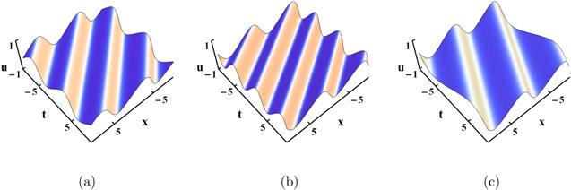 New window|Download| PPT slide