Hai-Li Li¹, Jing-Fei Zhang¹, Xin Zhang^,1,2,3,∗1College of Sciences & Ministry of Education's Key Laboratory of Data Analytics and Optimization for Smart Industry, Northeastern University, Shenyang 110819, China
²Center for High Energy Physics, Peking University, Beijing 100080, China
³Center for Gravitation and Cosmology, Yangzhou University, Yangzhou 225009, China

First author contact: ∗ Author to whom any correspondence should be addressed.
Received:2020-07-15Accepted:2020-08-4Online:2020-11-12


Abstract
In this work, we investigate the constraints on the total neutrino mass in the scenario of vacuum energy interacting with cold dark matter (abbreviated as IΛCDM) by using the latest cosmological observations. We consider four typical interaction forms, i.e. $Q=\beta H{\rho }_{\mathrm{de}}$, $Q=\beta H{\rho }_{{\rm{c}}}$, $Q=\beta {H}_{0}{\rho }_{\mathrm{de}}$, and $Q=\beta {H}_{0}{\rho }_{{\rm{c}}}$, in the IΛCDM scenario. To avoid the large-scale instability problem in interacting dark energy models, we employ the extended parameterized post-Friedmann method for interacting dark energy to calculate the perturbation evolution of dark energy in these models. The observational data used in this work include the cosmic microwave background (CMB) measurements from the Planck 2018 data release, the baryon acoustic oscillation (BAO) data, the type Ia supernovae (SN) observation (Pantheon compilation), and the 2019 local distance ladder measurement of the Hubble constant H₀ from the Hubble Space Telescope. We find that, compared with those in the ΛCDM+$\sum {m}_{\nu }$ model, the constrains on $\sum {m}_{\nu }$ are looser in the four IΛCDM+$\sum {m}_{\nu }$ models. When considering the three mass hierarchies of neutrinos, the constraints on $\sum {m}_{\nu }$ are tightest in the degenerate hierarchy case and loosest in the inverted hierarchy case. In addition, in the four IΛCDM+$\sum {m}_{\nu }$ models, the values of coupling parameter β are larger using the CMB+BAO+SN+H₀ data combination than that using the CMB+BAO+SN data combination, and β>0 is favored at more than 1σ level when using CMB+BAO+SN+H₀ data combination. The issue of the H₀ tension is also discussed in this paper. We find that, compared with the ΛCDM+$\sum {m}_{\nu }$ model, the H₀ tension can be alleviated in the IΛCDM+$\sum {m}_{\nu }$ model to some extent.
Keywords： total neutrino mass;neutrino mass hierarchies;interacting dark energy;Hubble tension;cosmological observations


PDF (748KB)MetadataMetricsRelated articlesExportEndNote|Ris|BibtexFavorite
Cite this article
Hai-Li Li, Jing-Fei Zhang, Xin Zhang. Constraints on neutrino mass in the scenario of vacuum energy interacting with cold dark matter after Planck 2018. Communications in Theoretical Physics, 2020, 72(12): 125401- doi:10.1088/1572-9494/abb7c9

1. Introduction

The phenomenon of neutrino oscillation indicates that neutrinos have nonzero masses and there are mass splittings between different neutrino species [1, 2]. The neutrino oscillation experiments can provide the information about the squared mass differences between the neutrino mass eigenstates. Specifically, the solar and reactor experiments give the result of ${\rm{\Delta }}{m}_{21}^{2}\simeq 7.5\times {10}^{-5}\,{\mathrm{eV}}^{2}$, and the atmospheric and accelerator beam experiments give the result of $| {\rm{\Delta }}{m}_{31}^{2}| \simeq 2.5\times {10}^{-3}\,{\mathrm{eV}}^{2}$ [2, 3]. Therefore, we can get two possible mass hierarchies of the neutrino mass spectrum, i.e. the normal hierarchy (NH) with m₁<m₂ ≪ m₃ and the inverted hierarchy (IH) with m₃ ≪ m₁<m₂, where m₁, m₂, and m₃ denote the masses of neutrinos for the three mass eigenstates. However, the absolute masses of neutrinos are still unknown.

In principle, laboratory experiments of particle physics can directly measure the absolute masses of neutrinos, but these experiments have always been facing great challenges [4-12]. Compared with these particle physics experiments, cosmological observations are more prone to be capable of measuring the absolute masses of neutrinos [13-15], since massive neutrinos can leave rich signatures on the cosmic microwave background (CMB) anisotropies and the large-scale structure (LSS) formation at different epochs of the cosmic evolution [16]. Thus, we can extract useful information on neutrinos from these available cosmological observations.

Recently, the issue of cosmological constraints on the total neutrino mass with the consideration of mass hierarchy using the latest observational data has been discussed in [17]. In [17], the authors discussed the constraints on neutrino mass in several typical dark energy (DE) models, e.g. the Λ cold dark matter (ΛCDM), wCDM, Chevallier-Polarski-Linder (CPL), and holographic dark energy (HDE) models. It was found that, compared to the ΛCDM+$\sum {m}_{\nu }$ model, larger neutrino masses are favored in the wCDM+$\sum {m}_{\nu }$ and CPL+$\sum {m}_{\nu }$ models, and the most stringent upper limits are obtained in the HDE+$\sum {m}_{\nu }$ model. Moreover, in [17], it was also confirmed that the NH case is more favored by current cosmological observations than the IH case. For more relevant studies on constraining the total neutrino mass by using cosmological observations, see e.g. [18-69].

Furthermore, the impacts of interaction between DE and cold dark matter (CDM) on constraining neutrino mass have also been considered. For example, in the scenario of vacuum energy interacting with cold dark matter, which is abbreviated as the IΛCDM scenario in this work, the constraint on $\sum {m}_{\nu }$ becomes $\sum {m}_{\nu }\lt 0.10\,\mathrm{eV}$ (2σ) for $Q=\beta H{\rho }_{\mathrm{de}}$, $\sum {m}_{\nu }\lt 0.20\,\mathrm{eV}$ (2σ) for $Q=\beta H{\rho }_{{\rm{c}}}$ [70], and $\sum {m}_{\nu }\lt 0.214\,\mathrm{eV}$ (2σ) for $Q=\beta {H}_{0}{\rho }_{{\rm{c}}}$ [71]. When the mass hierarchies of neutrinos are considered in the IΛCDM model [72, 73], the results showed that the degenerate hierarchy (DH) case gives the smallest upper limit of the neutrino mass and the NH case is more favored over the IH case. In the present work, we will revisit the constraints on the total neutrino mass in the IΛCDM scenario after the Planck 2018 data release. We will consider more forms of interaction term Q, and also adopt the mass hierarchies of neutrinos in this work.

In the so-called ‘interacting dark energy' (IDE) scenario, some direct, nongravitational coupling between DE and dark matter is assumed and its cosmological consequences have been widely studied [74-114]. Theoretically speaking, the consideration of such an interaction is helpful in solving the cosmic coincidence problem [76-78, 87, 89], but actually what is more important is to detect such an interaction using the cosmological observations. The impacts of interactions between DE and dark matter on the CMB [89, 106] and LSS [75, 83, 87, 90, 101, 106] have been studied in-depth.

In this paper, we only consider the simplest class of models in the IDE scenario, i.e. the IΛCDM models, in which the vacuum energy with w=−1 serves as DE. In this scenario, the energy conservation equations of the vacuum energy and the cold dark matter satisfy(1)$\begin{eqnarray}\dot{{\rho }_{\mathrm{de}}}=Q,\end{eqnarray}$(2)$\begin{eqnarray}\dot{{\rho }_{{\rm{c}}}}=-3H{\rho }_{{\rm{c}}}-Q,\end{eqnarray}$where ρ_de and ρ_c represent the densities of DE (namely, vacuum energy) and cold dark matter, respectively, H is the Hubble parameter, the dot represents the derivative with respect to the cosmic time t, and Q is the energy transfer rate. Usually, the form of Q is assumed to be proportional to the density of DE or dark matter, i.e. $Q=\beta H{\rho }_{\mathrm{de}}$ or $Q=\beta H{\rho }_{{\rm{c}}}$, where the appearance of H is only for mathematical convenience. In the research area of IDE, another perspective is to consider $Q=\beta {H}_{0}{\rho }_{\mathrm{de}}$ or $Q=\beta {H}_{0}{\rho }_{{\rm{c}}}$ [86], where the appearance of H₀ is only for a dimensional consideration. From equations (1) and (2), it is known that β>0 means cold dark matter decaying into DE, β<0 means DE decaying into cold dark matter, and β=0 indicates no interaction between vacuum energy and cold dark matter.

Different phenomenological models of IΛCDM can be built by assuming different forms of Q. In this work, we will collect the popular forms of Q in the current literature and then focus on the impacts of different forms of Q on constraining the total neutrino mass after the Planck 2018 data release. We will consider the four typical forms of Q: $Q=\beta H{\rho }_{\mathrm{de}}$, $Q=\beta H{\rho }_{{\rm{c}}}$, $Q=\beta {H}_{0}{\rho }_{\mathrm{de}}$ and $Q=\beta {H}_{0}{\rho }_{{\rm{c}}}$. The mass hierarchies of neutrinos are also considered in this work. In addition, we also wish to see whether some hint of the existence of nonzero interaction can be found in these IΛCDM models by using the latest observational data.

This paper is organized as follows. In section 2, we introduce the cosmological observations used in this work and briefly describe the analysis method. In section 3, we report the constraint results and then make some relevant discussions. The issue of H₀ tension will also be discussed in this section. Conclusion is given in section 4.

2. Method and data

In the IΛCDM model, there are seven basic cosmological parameters $\{{\omega }_{b},\,{\omega }_{c},\,100{\theta }_{\mathrm{MC}},\,\tau ,\,{n}_{s},\,\mathrm{ln}({10}^{10}{A}_{s}),\beta \}$, where ω_b is the present density of baryons, ω_c is the present density of cold dark matter, θ_MC is the ratio between the sound horizon to the angular diameter distance at the decoupling epoch, τ is the Thomson scattering optical depth to reionization, n_s is the scalar spectral index, A_s is the amplitude of primordial scalar perturbation power spectrum, and β is the dimensionless coupling constant describing the coupling strength between vacuum energy and dark matter.

For the IΛCDM model there is a problem of early-time perturbation instability, because in the IDE models, the cosmological perturbations of DE will be divergent in a part of the parameter space, which ruins the IDE cosmology in the perturbation level. The origin of the difficulty is that we know little about the nature of DE, so we do not know how to treat the spread of sounds in DE fluid which has a negative equation of state. To overcome the problem of perturbation instability, in 2014, Yun-He Li, Jing-Fei Zhang, and Xin Zhang established an effective theoretical framework for IDE cosmology based on the extended version of the parameterized post-Friedmann (PPF) approach, which can safely calculate the cosmological perturbations in the whole parameter space of an IDE model. About the extended PPF method, see [115-119], and the original PPF method is introduced in [120, 121]. In this work, we will employ the extended PPF method [115-119] to calculate the cosmological perturbations in the IΛCDM model.

We use the modified version of the publicly available Markov-chain Monte Carlo package CosmoMC [122] to constrain the neutrino mass and other cosmological parameters. We monitor the convergence of the generated MCMC chains by using the Gelman-Rubin parameter R [123], requiring $R-1\lt 0.01$ for our MCMC chains to be considered as converged. When considering the neutrino mass splitting, we should note the following rules. For the NH case, the neutrino mass spectrum is(3)$\begin{eqnarray}({m}_{1},{m}_{2},{m}_{3})=({m}_{1},\sqrt{{m}_{1}^{2}+{\rm{\Delta }}{m}_{21}^{2}},\sqrt{{m}_{1}^{2}+| {\rm{\Delta }}{m}_{31}^{2}| }),\end{eqnarray}$where m₁ is a free parameter; for the IH case, the neutrino mass spectrum is(4)$\begin{eqnarray}\begin{array}{l}({m}_{1},{m}_{2},{m}_{3})\\ \quad =\,(\sqrt{{m}_{3}^{2}+| {\rm{\Delta }}{m}_{31}^{2}| },\sqrt{{m}_{3}^{2}+| {\rm{\Delta }}{m}_{31}^{2}| +{\rm{\Delta }}{m}_{21}^{2}},{m}_{3}),\end{array}\end{eqnarray}$where m₃ is a free parameter; for comparison, the DH case is also considered, in which the neutrino mass spectrum is(5)$\begin{eqnarray}{m}_{1}={m}_{2}={m}_{3}=m,\end{eqnarray}$where m is a free parameter. Since we have two values of squared mass differences, ${\rm{\Delta }}{m}_{21}^{2}=7.5\times {10}^{-5}\,{\mathrm{eV}}^{2}$ and $| {\rm{\Delta }}{m}_{31}^{2}| =2.5\times {10}^{-3}\,{\mathrm{eV}}^{2}$ [2, 3], the lower limits of NH and IH can be derived by setting the smallest mass be zero. Thus, the input lower bounds of $\sum {m}_{\nu }$ are 0.06 eV for the NH case, 0.10 eV for the IH case, and 0 eV for the DH case, respectively.

The current observational data sets we used in this paper include CMB, BAO, SN and H₀. For the CMB data, we use the Planck TT, TE, EE spectra at ℓ≥30, the low-ℓ temperature Commander likelihood, and the low-ℓ SimAll EE likelihood, from the Planck 2018 data release [124]. For the BAO data, we consider the measurements from 6dFGS (z_eff=0.106) [125], SDSS-MGS (z_eff=0.15) [126], and BOSS DR12 (z_eff=0.38, 0.51, and 0.61) [127]. For the SN data, we employ the latest Pantheon sample, which is comprised of 1048 data points from the Pantheon compilation [128]. For the H₀ data, we use the 2019 local distance ladder measurement of the Hubble constant ${H}_{0}=74.03\pm 1.42\,\mathrm{km}\,{{\rm{s}}}^{-1}\,{\mathrm{Mpc}}^{-1}$ from the Hubble Space Telescope [129]. In our analysis, we will use two data combinations, i.e. CMB+BAO+SN and CMB+BAO+SN+H₀, to constrain the cosmological parameters.

3. Results and discussion

In this section, we report the constraint results of cosmological parameters for these IΛCDM+$\sum {m}_{\nu }$ models. The fitting results are listed in table 1 for the ΛCDM+$\sum {m}_{\nu }$ model and tables 2-5 and figures 1-4 for the four IΛCDM+$\sum {m}_{\nu }$ models. For convenience, the IΛCDM models with the interaction terms $Q=\beta H{\rho }_{\mathrm{de}}$, $Q=\beta H{\rho }_{{\rm{c}}}$, $Q=\beta {H}_{0}{\rho }_{\mathrm{de}}$ and $Q=\beta {H}_{0}{\rho }_{{\rm{c}}}$ are denoted as ‘IΛCDM1', ‘IΛCDM2', ‘IΛCDM3', and ‘IΛCDM4', respectively. In these tables, we show the best fit values with ±1σ errors of the cosmological parameters, but for the total neutrino mass $\sum {m}_{\nu }$, which cannot be well constrained, the 2σ upper limits are given.

Figure 1.

New window|Download| PPT slide
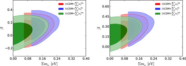
Figure 1.Observational constraints (68.3% and 95.4% confidence level) on the IΛCDM1+$\sum {m}_{\nu }$ ($Q=\beta H{\rho }_{\mathrm{de}}$) model by using the CMB+BAO+SN (left) and CMB+BAO+SN+H₀ (right) data combinations, respectively.

Figure 2.

New window|Download| PPT slide
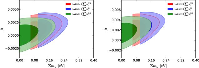
Figure 2.Observational constraints (68.3% and 95.4% confidence level) on the IΛCDM2+$\sum {m}_{\nu }$ ($Q=\beta H{\rho }_{{\rm{c}}}$) model by using the CMB+BAO+SN (left) and CMB+BAO+SN+H₀ (right) data combinations, respectively.

Figure 3.

New window|Download| PPT slide
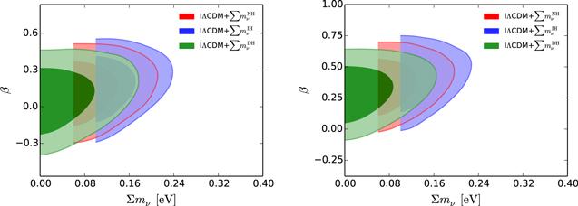
Figure 3.Observational constraints (68.3% and 95.4% confidence level) on the IΛCDM3+$\sum {m}_{\nu }$ ($Q=\beta {H}_{0}{\rho }_{\mathrm{de}}$) model by using the CMB+BAO+SN (left) and CMB+BAO+SN+H₀ (right) data combinations, respectively.

Figure 4.

New window|Download| PPT slide
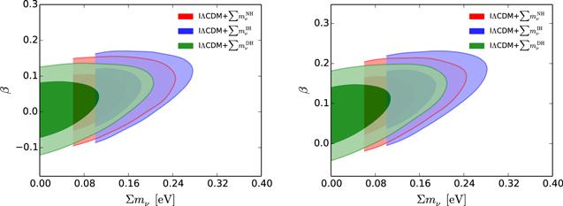
Figure 4.Observational constraints (68.3% and 95.4% confidence level) on the IΛCDM4+$\sum {m}_{\nu }$ ($Q=\beta {H}_{0}{\rho }_{{\rm{c}}}$) model by using the CMB+BAO+SN (left) and CMB+BAO+SN+H₀ (right) data combinations, respectively.



Table 1.
Table 1.Fitting results for the ΛCDM+$\sum {m}_{\nu }$ model by using the CMB+BAO+SN and CMB+BAO+SN+H₀ data combinations, respectively. Here, H₀ and $\sum {m}_{\nu }$ are in units of km s⁻¹ Mpc⁻¹ and eV, respectively.

Data	CMB+BAO+SN			CMB+BAO+SN+H0
Model	ΛCDM+$\sum {m}_{\nu }^{\mathrm{NH}}$	ΛCDM+$\sum {m}_{\nu }^{\mathrm{IH}}$	ΛCDM+$\sum {m}_{\nu }^{\mathrm{DH}}$	ΛCDM+$\sum {m}_{\nu }^{\mathrm{NH}}$	ΛCDM+$\sum {m}_{\nu }^{\mathrm{IH}}$	ΛCDM+$\sum {m}_{\nu }^{\mathrm{DH}}$
Ωm	0.3126±0.0063	0.3150±0.0060	0.3097±0.0063	0.3044±0.0056	0.3069±0.0056	0.3015±0.0056
${H}_{0}$	67.48±0.47	67.26±0.45	67.75±0.49	68.11±0.43	67.88±0.43	68.40±0.44
σ8	${0.801}_{-0.008}^{+0.011}$	${0.793}_{-0.008}^{+0.010}$	${0.812}_{-0.008}^{+0.013}$	${0.801}_{-0.008}^{+0.009}$	${0.792}_{-0.008}^{+0.009}$	${0.813}_{-0.008}^{+0.010}$
$\sum {m}_{\nu }$	$\lt 0.156$	$\lt 0.185$	<0.123	<0.125	<0.160	<0.082

New window|CSV


Table 2.
Table 2.Fitting results for the IΛCDM1+$\sum {m}_{\nu }$ ($Q=\beta H{\rho }_{\mathrm{de}}$) model by using the CMB+BAO+SN and CMB+BAO+SN+H₀ data combinations, respectively. Here, H₀ and $\sum {m}_{\nu }$ are in units of km s⁻¹ Mpc⁻¹ and eV, respectively.

Data	CMB+BAO+SN			CMB+BAO+SN+H0
Model	IΛCDM+$\sum {m}_{\nu }^{\mathrm{NH}}$	IΛCDM+$\sum {m}_{\nu }^{\mathrm{IH}}$	IΛCDM+$\sum {m}_{\nu }^{\mathrm{DH}}$	IΛCDM+$\sum {m}_{\nu }^{\mathrm{NH}}$	IΛCDM+$\sum {m}_{\nu }^{\mathrm{IH}}$	IΛCDM+$\sum {m}_{\nu }^{\mathrm{DH}}$
Ωm	0.285±0.029	0.279±0.030	${0.292}_{-0.030}^{+0.029}$	0.235±0.027	0.229±0.027	${0.243}_{-0.027}^{+0.028}$
${H}_{0}$	68.08±0.81	${68.08}_{-0.82}^{+0.83}$	68.14±0.83	${69.64}_{-0.72}^{+0.73}$	${69.62}_{-0.73}^{+0.75}$	${69.67}_{-0.75}^{+0.74}$
β	${0.10}_{-0.11}^{+0.10}$	0.13±0.11	${0.07}_{-0.11}^{+0.10}$	${0.257}_{-0.097}^{+0.096}$	0.286±0.098	0.215±0.099
${\sigma }_{8}$	${0.870}_{-0.088}^{+0.058}$	${0.884}_{-0.094}^{+0.061}$	${0.859}_{-0.085}^{+0.056}$	${1.013}_{-0.123}^{+0.076}$	${1.031}_{-0.131}^{+0.081}$	${0.987}_{-0.117}^{+0.073}$
$\sum {m}_{\nu }$	<0.189	<0.218	<0.151	<0.177	<0.209	<0.138

New window|CSV

3.1. Neutrino mass

Firstly, we use the CMB+BAO+SN data combination to constrain these models. In the ΛCDM+$\sum {m}_{\nu }$ model, we obtain $\sum {m}_{\nu }\lt 0.156\,\mathrm{eV}$ for the NH case, $\sum {m}_{\nu }\lt 0.185\,\mathrm{eV}$ for the IH case, and $\sum {m}_{\nu }\lt 0.123\,\mathrm{eV}$ for the DH case, as shown table 1. In the IΛCDM1+$\sum {m}_{\nu }$ model, the constraint results are $\sum {m}_{\nu }\lt 0.187\,\mathrm{eV}$ for the NH case, $\sum {m}_{\nu }\,\lt 0.218\,\mathrm{eV}$ for the IH case, and $\sum {m}_{\nu }\lt 0.151\,\mathrm{eV}$ for the DH case (see table 2); in the IΛCDM2+$\sum {m}_{\nu }$ model, the results are $\sum {m}_{\nu }\lt 0.190\,\mathrm{eV}$ for the NH case, $\sum {m}_{\nu }\lt 0.223\,\mathrm{eV}$ for the IH case, and $\sum {m}_{\nu }\lt 0.149\,\mathrm{eV}$ for the DH case (see table 3); in the IΛCDM3+$\sum {m}_{\nu }$ model, we get $\sum {m}_{\nu }\lt 0.179\,\mathrm{eV}$ for the NH case, $\sum {m}_{\nu }\lt 0.208\,\mathrm{eV}$ for the IH case, and $\sum {m}_{\nu }\lt 0.140\,\mathrm{eV}$ for the DH case (see table 4); in the IΛCDM4+$\sum {m}_{\nu }$ model, the constraint results become $\sum {m}_{\nu }\lt 0.202\,\mathrm{eV}$ for the NH case, $\sum {m}_{\nu }\lt 0.235\,\mathrm{eV}$ for the IH case, and $\sum {m}_{\nu }\lt 0.156\,\mathrm{eV}$ for the DH case (see table 5). We find that, the constraint results of $\sum {m}_{\nu }$ are looser in the four IΛCDM+$\sum {m}_{\nu }$ models than those in the ΛCDM+$\sum {m}_{\nu }$ model. When considering the three mass hierarchies, we find that the constraint results of $\sum {m}_{\nu }$ are tightest in the DH case and loosest in the IH case (see the left panels in figures 1-4); actually this is mainly because in the NH and IH cases there are lower limits for the total neutrino mass.


Table 3.
Table 3.Fitting results for the IΛCDM2+$\sum {m}_{\nu }$ (Q=β H ρ_c) model by using the CMB+BAO+SN and CMB+BAO+SN+H₀ data combinations, respectively. Here, H₀ and $\sum {m}_{\nu }$ are in units of km s⁻¹ Mpc⁻¹ and eV, respectively.

Data	CMB+BAO+SN			CMB+BAO+SN+H0
Model	IΛCDM+$\sum {m}_{\nu }^{\mathrm{NH}}$	IΛCDM+$\sum {m}_{\nu }^{\mathrm{IH}}$	IΛCDM+$\sum {m}_{\nu }^{\mathrm{DH}}$	IΛCDM+$\sum {m}_{\nu }^{\mathrm{NH}}$	IΛCDM+$\sum {m}_{\nu }^{\mathrm{IH}}$	IΛCDM+$\sum {m}_{\nu }^{\mathrm{DH}}$
${{\rm{\Omega }}}_{{\rm{m}}}$	0.3085±0.0080	0.3092±0.0081	0.3077±0.0081	0.2953±0.0071	${0.2960}_{-0.0072}^{+0.0071}$	${0.2946}_{-0.0072}^{+0.0071}$
${H}_{0}$	67.83±0.64	67.74±0.65	67.92±0.65	68.92±0.60	${68.83}_{-0.60}^{+0.61}$	${69.01}_{-0.60}^{+0.61}$
β	${0.0011}_{-0.0012}^{+0.0013}$	${0.0014}_{-0.0013}^{+0.0012}$	0.0005±0.0013	0.0024±0.0012	0.0028±0.0012	0.0019±0.0012
${\sigma }_{8}$	${0.806}_{-0.012}^{+0.014}$	${0.800}_{-0.012}^{+0.014}$	${0.814}_{-0.013}^{+0.014}$	${0.815}_{-0.012}^{+0.013}$	${0.809}_{-0.012}^{+0.013}$	${0.824}_{-0.012}^{+0.014}$
$\sum {m}_{\nu }$	$\lt 0.190$	<0.223	<0.149	<0.170	<0.202	<0.126

New window|CSV


Table 4.
Table 4.Fitting results for the IΛCDM3+$\sum {m}_{\nu }$ ($Q=\beta {H}_{0}{\rho }_{\mathrm{de}}$) model by using the CMB+BAO+SN and CMB+BAO+SN+H₀ data combinations, respectively. Here, H₀ and $\sum {m}_{\nu }$ are in units of km s⁻¹ Mpc⁻¹ and eV, respectively.

Data	CMB+BAO+SN			CMB+BAO+SN+H0
Model	IΛCDM+$\sum {m}_{\nu }^{\mathrm{NH}}$	IΛCDM+$\sum {m}_{\nu }^{\mathrm{IH}}$	IΛCDM+$\sum {m}_{\nu }^{\mathrm{DH}}$	IΛCDM+$\sum {m}_{\nu }^{\mathrm{NH}}$	IΛCDM+$\sum {m}_{\nu }^{\mathrm{IH}}$	IΛCDM+$\sum {m}_{\nu }^{\mathrm{DH}}$
Ωm	${0.282}_{-0.035}^{+0.036}$	0.276±0.035	0.291±0.036	${0.223}_{-0.031}^{+0.032}$	0.217±0.033	0.233±0.032
${H}_{0}$	68.03±0.81	${67.96}_{-0.80}^{+0.79}$	68.10±0.83	69.57±0.72	69.50±0.74	${69.63}_{-0.72}^{+0.73}$
β	0.14±0.16	0.18±0.16	${0.08}_{-0.17}^{+0.16}$	${0.37}_{-0.14}^{+0.13}$	0.40±0.14	0.31±0.14
${\sigma }_{8}$	${0.886}_{-0.118}^{+0.069}$	${0.899}_{-0.122}^{+0.072}$	${0.868}_{-0.113}^{+0.068}$	${1.072}_{-0.172}^{+0.095}$	${1.10}_{-0.19}^{+0.10}$	${1.036}_{-0.156}^{+0.091}$
$\sum {m}_{\nu }$	$\lt 0.179$	<0.208	<0.140	<0.166	<0.198	<0.128

New window|CSV


Table 5.
Table 5.Fitting results for the IΛCDM4+$\sum {m}_{\nu }$ ($Q=\beta {H}_{0}{\rho }_{{\rm{c}}}$) model by using the CMB+BAO+SN and CMB+BAO+SN+H₀ data combinations, respectively. Here, H₀ and $\sum {m}_{\nu }$ are in units of km s⁻¹ Mpc⁻¹ and eV, respectively.

Data	CMB+BAO+SN			CMB+BAO+SN+H0
Model	IΛCDM+$\sum {m}_{\nu }^{\mathrm{NH}}$	IΛCDM+$\sum {m}_{\nu }^{\mathrm{IH}}$	IΛCDM+$\sum {m}_{\nu }^{\mathrm{DH}}$	IΛCDM+$\sum {m}_{\nu }^{\mathrm{NH}}$	IΛCDM+$\sum {m}_{\nu }^{\mathrm{IH}}$	IΛCDM+$\sum {m}_{\nu }^{\mathrm{DH}}$
${{\rm{\Omega }}}_{{\rm{m}}}$	0.299±0.016	0.297±0.016	${0.302}_{-0.017}^{+0.016}$	0.272±0.013	0.269±0.013	0.275±0.013
${H}_{0}$	68.05±0.80	${68.07}_{-0.82}^{+0.83}$	68.07±0.81	69.58±0.72	69.58±0.73	${69.58}_{-0.72}^{+0.71}$
β	0.043±0.047	${0.058}_{-0.048}^{+0.047}$	${0.024}_{-0.048}^{+0.047}$	0.111±0.043	0.128±0.043	0.092±0.044
${\sigma }_{8}$	${0.814}_{-0.021}^{+0.019}$	0.812±0.019	${0.820}_{-0.020}^{+0.019}$	0.840±0.019	0.837±0.019	0.845±0.019
$\sum {m}_{\nu }$	$\lt 0.202$	$\lt 0.235$	<0.156	<0.202	<0.239	<0.162

New window|CSV

Then, we consider the data combination involving the latest local measurement of the Hubble constant H₀ to constrain these models. By using the CMB+BAO+SN+H₀ data combination, we find that the constraint results of $\sum {m}_{\nu }$ are looser in the four IΛCDM+$\sum {m}_{\nu }$ models than those in the ΛCDM+$\sum {m}_{\nu }$ model, and when considering the three mass hierarchies, the constraint results of $\sum {m}_{\nu }$ are tightest in the DH case and loosest in the IH case. These conclusions are consistent with the case using the CMB+BAO+SN data combination. Additionally, we also find that the constraints on $\sum {m}_{\nu }$ become slightly tighter for using CMB+BAO+SN+H₀ than CMB+BAO+SN.

3.2. Coupling parameter

In this subsection, we discuss the fitting results of the coupling parameter β in these four IΛCDM+$\sum {m}_{\nu }$ models by using the CMB+BAO+SN and CMB+BAO+SN+H₀ data combinations, respectively.

First, we constrain the IΛCDM1+$\sum {m}_{\nu }$ model (see table 2) using the CMB+BAO+SN data combination, and we obtain $\beta ={0.10}_{-0.11}^{+0.10}$ for the NH case, β=0.13±0.11 for the IH case, and $\beta ={0.07}_{-0.11}^{+0.10}$ for the DH case. It is shown that a positive value of β is favored and β>0 is at the 0.91σ, 1.18σ, and 0.64σ levels for the three mass hierarchy cases, respectively. Furthermore, we constrain this model by using the CMB+BAO+SN+H₀ data combination, and we obtain $\beta ={0.257}_{-0.097}^{+0.096}$ for the NH case, β=0.286±0.098 for the IH case, and β=0.215±0.099 for the DH case. Now, β>0 is obtained at the 2.65σ, 2.92σ, and 2.17σ levels, respectively. This indicates that cold dark matter decaying into DE is favored when using the CMB+BAO+SN+H₀ data combination.

For the IΛCDM2+$\sum {m}_{\nu }$ model (see table 3), we obtain $\beta ={0.0011}_{-0.0012}^{+0.0013}$ for the NH case, $\beta ={0.0014}_{-0.0013}^{+0.0012}$ for the IH case, and $\beta =0.0005\pm 0.0013$ for the DH case, by using the CMB+BAO+SN data combination. Thus, β>0 is favored at the 0.92σ, 1.08σ, and 0.38σ levels, respectively. When using the CMB+BAO+SN+H₀ data combination, we obtain β=0.0024±0.0012 for the NH case, β=0.0028±0.0012 for the IH case, and β=0.0019±0.0012 for the DH case, which indicates that a positive value of β can be detected at the 2.00σ, 2.33σ, and 1.58σ levels, respectively.

As for the IΛCDM3+$\sum {m}_{\nu }$ model (see table 4), we obtain β=0.14±0.16 for the NH case, β=0.18±0.16 for the IH case, and $\beta ={0.08}_{-0.17}^{+0.16}$ for the DH case, by using the CMB+BAO+SN data combination. Therefore, the positive values of β are favored and β>0 is preferred at the 0.88σ, 1.13σ, and 0.50σ levels, respectively. When using the CMB+BAO+SN+H₀ data combination, we obtain $\beta ={0.37}_{-0.14}^{+0.13}$ for the NH case, β=0.40±0.14 for the IH case, and β=0.31±0.14 for the DH case, respectively. And β>0 is detected at the 2.64σ, 2.90σ, and 2.21σ levels, respectively, which indicates cold dark matter decaying into DE.

Finally, we show the constraint results of IΛCDM4+$\sum {m}_{\nu }$ model (see table 5). We obtain β=0.043±0.047 for the NH case, $\beta ={0.058}_{-0.048}^{+0.047}$ for the IH case, and $\beta ={0.024}_{-0.048}^{+0.047}$ for the DH case, by using the CMB+BAO+SN data combination. So, a positive value of β is favored and β>0 is at the 0.91σ, 1.21σ, and 0.50σ levels, respectively. When using the CMB+BAO+SN+H₀ data combination, we obtain β=0.111±0.043 for the NH case, β=0.128±0.043 for the IH case, and β=0.092±0.044 for the DH case. Now, β>0 is preferred at the 2.58σ, 2.98σ, and 2.09σ levels, respectively. The conclusion is the same as the above three cases, i.e. cold dark matter decaying into DE is supported by the CMB+BAO+SN+H₀ data combination.

In summary, for all the IΛCDM+$\sum {m}_{\nu }$ models considered in this paper, the values of β are greater by using the CMB+BAO+SN+H₀ data combination than using CMB+BAO+SN data combination. We can also intuitively obtain this conclusion by comparing the left and right panels of figures 1-4. Additionally, when using CMB+BAO+SN+H₀ data combination, β>0 is favored at more than 1σ level in all the IΛCDM+$\sum {m}_{\nu }$ models, which indicates that cold dark matter decaying into DE is supported in these models.

3.3. The H₀ tension

In this subsection, we discuss the issue of H₀ tension between the Planck observation of the CMB power spectra and the local measurement based on the method of distance ladder. In the IΛCDM scenario, β>0 (in the convention defined in this work) leads to the vacuum energy behaving as an effective phantom, and thus a larger cosmic expansion rate compared with ΛCDM can be obtained. We therefore can use this scenario to discuss the issue of relaxing the Hubble tension. The detailed fitting results are given in tables 1-5 and figures 5-7.

Figure 5.

New window|Download| PPT slide
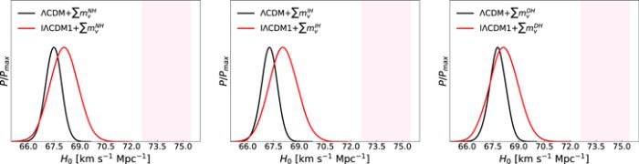
Figure 5.The one-dimensional posterior distributions for the parameter H₀ for the ΛCDM+$\sum {m}_{\nu }$ (NH, IH, and DH) model and IΛCDM1+$\sum {m}_{\nu }$ (NH, IH, and DH) model with $Q=\beta H{\rho }_{\mathrm{de}}$ by using the CMB+BAO+SN data combination. The result of the local measurement of Hubble constant (${H}_{0}=74.03\pm 1.42\,\mathrm{km}\,{{\rm{s}}}^{-1}\,{\mathrm{Mpc}}^{-1}$) is shown by the hotpink band.


In table 1, we show the constraint results of the ΛCDM+$\sum {m}_{\nu }$ model by using the CMB+BAO+SN data combination. We obtain ${H}_{0}=67.48\pm 0.47\,\mathrm{km}\,{{\rm{s}}}^{-1}\,{\mathrm{Mpc}}^{-1}$ for the NH case, ${H}_{0}=67.26\pm 0.45\,\mathrm{km}\,{{\rm{s}}}^{-1}\,{\mathrm{Mpc}}^{-1}$ for the IH case, and ${H}_{0}=67.75\pm 0.49\,\mathrm{km}\,{{\rm{s}}}^{-1}\,{\mathrm{Mpc}}^{-1}$ for the DH case, which are 4.38σ 4.54σ and 4.18σ lower than the direct measurement of the Hubble constant (${H}_{0}=74.03\,\pm 1.42\,\mathrm{km}\,{{\rm{s}}}^{-1}\,{\mathrm{Mpc}}^{-1}$). So, we investigate whether the H₀ tension can be solved or relieved in the IDE scenario. In tables 2-5, we show the constraint results of the IΛCDM1+$\sum {m}_{\nu }$, IΛCDM2+$\sum {m}_{\nu }$, IΛCDM3+$\sum {m}_{\nu }$, and IΛCDM4+$\sum {m}_{\nu }$ models from the CMB+BAO+SN data combination. In the IΛCDM1+$\sum {m}_{\nu }$ model, we obtain ${H}_{0}\,=68.08\,\pm 0.81\,\mathrm{km}\,{{\rm{s}}}^{-1}\,{\mathrm{Mpc}}^{-1}$ for the NH case, ${H}_{0}\,={68.08}_{-0.82}^{+0.83}\,\mathrm{km}\,{{\rm{s}}}^{-1}\,{\mathrm{Mpc}}^{-1}$ for the IH case, and ${H}_{0}=68.14\,\pm 0.83\,\mathrm{km}\,{{\rm{s}}}^{-1}\,{\mathrm{Mpc}}^{-1}$ for the DH case; in the IΛCDM2+$\sum {m}_{\nu }$ model, we obtain ${H}_{0}=67.83\pm 0.64\,\mathrm{km}\,{{\rm{s}}}^{-1}\,{\mathrm{Mpc}}^{-1}$ for the NH case, ${H}_{0}=67.74\pm 0.65\,\mathrm{km}\,{{\rm{s}}}^{-1}\,{\mathrm{Mpc}}^{-1}$ for the IH case, and ${H}_{0}=67.92\pm 0.65\,\mathrm{km}\,{{\rm{s}}}^{-1}\,{\mathrm{Mpc}}^{-1}$ for the DH case; in the IΛCDM3+$\sum {m}_{\nu }$ model, we obtain ${H}_{0}=68.03\,\pm 0.81\,\mathrm{km}\,{{\rm{s}}}^{-1}\,{\mathrm{Mpc}}^{-1}$ for the NH case, ${H}_{0}={67.96}_{-0.80}^{+0.79}\,\mathrm{km}\,{{\rm{s}}}^{-1}{\mathrm{Mpc}}^{-1}$ for the IH case, and ${H}_{0}=68.10\,\pm 0.83\,\mathrm{km}\,{{\rm{s}}}^{-1}\,{\mathrm{Mpc}}^{-1}$ for the DH case; in the IΛCDM4+$\sum {m}_{\nu }$ model, we obtain ${H}_{0}=68.05\pm 0.80\,\mathrm{km}\,{{\rm{s}}}^{-1}\,{\mathrm{Mpc}}^{-1}$ for the NH case, ${H}_{0}={68.07}_{-0.82}^{+0.83}\,\mathrm{km}\,{{\rm{s}}}^{-1}\,{\mathrm{Mpc}}^{-1}$ for the IH case, and ${H}_{0}=68.07\,\pm 0.81\,\mathrm{km}\,{{\rm{s}}}^{-1}\,{\mathrm{Mpc}}^{-1}$ for the DH case. For these cases, the tensions with the Hubble constant direct measurement are at the 3.64σ level, 3.62σ level, 3.58σ level, 3.98σ level, 4.03σ level, 3.91σ level, 3.67σ level, 3.74σ level, 3.61σ level, 3.67σ level, 3.62σ level, and 3.65σ level, respectively.

Then, we show the constraint results of these models by using the CMB+BAO+SN+H₀ data combination (see tables 1-5). In the ΛCDM+$\sum {m}_{\nu }$ model, we obtain ${H}_{0}=68.11\,\pm 0.43\,\mathrm{km}\,{{\rm{s}}}^{-1}\,{\mathrm{Mpc}}^{-1}$ for the NH case, ${H}_{0}=67.88\,\pm 0.43\,\mathrm{km}\,{{\rm{s}}}^{-1}\,{\mathrm{Mpc}}^{-1}$ for the IH case, and ${H}_{0}=68.40\,\pm 0.44\,\mathrm{km}\,{{\rm{s}}}^{-1}\,{\mathrm{Mpc}}^{-1}$ for the DH case, which indicates that the tensions with the Hubble constant direct measurement are at the 3.99σ level 4.14σ level and 3.79σ level, respectively. In the IΛCDM1+$\sum {m}_{\nu }$ model, we obtain ${H}_{0}={69.64}_{-0.72}^{+0.73}\,\mathrm{km}\,{{\rm{s}}}^{-1}\,{\mathrm{Mpc}}^{-1}$ for the NH case, ${H}_{0}\,={69.62}_{-0.73}^{+0.75}\,\mathrm{km}\,{{\rm{s}}}^{-1}\,{\mathrm{Mpc}}^{-1}$ for the IH case, and ${H}_{0}\,={69.67}_{-0.75}^{+0.74}\,\mathrm{km}\,{{\rm{s}}}^{-1}\,{\mathrm{Mpc}}^{-1}$ for the DH case; in the IΛCDM2+$\sum {m}_{\nu }$ model, we obtain ${H}_{0}=68.92\,\pm 0.60\,\mathrm{km}\,{{\rm{s}}}^{-1}\,{\mathrm{Mpc}}^{-1}$ for the NH case, ${H}_{0}={68.83}_{-0.60}^{+0.61}\,\mathrm{km}\,{{\rm{s}}}^{-1}{\mathrm{Mpc}}^{-1}$ for the IH case, and ${H}_{0}={69.01}_{-0.60}^{+0.61}\,\mathrm{km}\,{{\rm{s}}}^{-1}\,{\mathrm{Mpc}}^{-1}$ for the DH case; in the IΛCDM3+$\sum {m}_{\nu }$ model, we obtain ${H}_{0}=69.57\,\pm 0.72\,\mathrm{km}\,{{\rm{s}}}^{-1}\,{\mathrm{Mpc}}^{-1}$ for the NH case, ${H}_{0}\,=69.50\pm 0.74\,\mathrm{km}\,{{\rm{s}}}^{-1}\,{\mathrm{Mpc}}^{-1}$ for the IH case, and ${H}_{0}\,={69.63}_{-0.72}^{+0.73}\,\mathrm{km}{{\rm{s}}}^{-1}\,{\mathrm{Mpc}}^{-1}$ for the DH case; in the IΛCDM4+$\sum {m}_{\nu }$ model, we obtain ${H}_{0}=69.58\pm 0.72\,\mathrm{km}\,{{\rm{s}}}^{-1}\,{\mathrm{Mpc}}^{-1}$ for the NH case, ${H}_{0}=69.58\pm 0.73\,\mathrm{km}\,{{\rm{s}}}^{-1}\,{\mathrm{Mpc}}^{-1}$ for the IH case, and ${H}_{0}={69.58}_{-0.72}^{+0.71}\,\mathrm{km}\,{{\rm{s}}}^{-1}\,{\mathrm{Mpc}}^{-1}$ for the DH case. The tensions with the Hubble constant direct measurement are at the 2.75σlevel, 2.75σ level, 2.72σ level, 3.31σ level, 3.36σ level, 3.25σ level, 2.80σ level, 2.83σ level, 2.76σ level, 2.80σ level, 2.79σ level, and 2.80σ level, respectively.

From the above constraint results, we find that compared with the ΛCDM+$\sum {m}_{\nu }$ model, the H₀ tension can indeed be relieved in the IΛCDM+$\sum {m}_{\nu }$ model. From figures 5, 6 we can clearly see that for whichever neutrino mass hierarchy case, the fitting values of H₀ in the IΛCDM+$\sum {m}_{\nu }$ models (here, we take IΛCDM1+$\sum {m}_{\nu }$ with $Q=\beta H{\rho }_{\mathrm{de}}$ as an example) are always much larger than those in the ΛCDM+$\sum {m}_{\nu }$ model. We also find that, the CMB+BAO+SN+H₀ data combination (about $2.7-3.4\sigma $ level) is slightly more effective in relieving the H₀ tension than the CMB+BAO+SN data combination (about $3.6-4.0\sigma $ level), due to the employment of the H₀ prior in the data combination. To visually display the result, we also take the IΛCDM1+$\sum {m}_{\nu }$ model as an example to give this result in figure 7. From these figures, we can clearly see that for whichever hierarchy of the neutrino mass spectrum, the values of H₀ are always much larger when adding the H₀ data in a cosmological fit. Certainly, the H₀ tension problem only can be alleviated to some extent in these cases, but cannot be truly solved. For the issue of H₀ tension, further exploration is needed.

Figure 6.

New window|Download| PPT slide
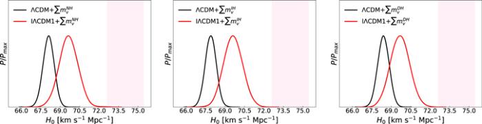
Figure 6.The one-dimensional posterior distributions for the parameter H₀ for the ΛCDM+$\sum {m}_{\nu }$ (NH, IH, and DH) model and IΛCDM1+$\sum {m}_{\nu }$ (NH, IH, and DH) model with $Q=\beta H{\rho }_{\mathrm{de}}$ by using the CMB+BAO+SN+H₀ data combination. The result of the local measurement of Hubble constant (${H}_{0}=74.03\pm 1.42\,\mathrm{km}\,{{\rm{s}}}^{-1}\,{\mathrm{Mpc}}^{-1}$) is shown by the hotpink band.

Figure 7.

New window|Download| PPT slide
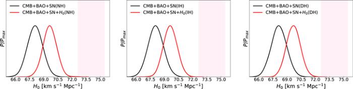
Figure 7.The one-dimensional posterior distributions for the parameter H₀ for the IΛCDM1+$\sum {m}_{\nu }$ (NH, IH, and DH) model with $Q=\beta H{\rho }_{\mathrm{de}}$ by using the CMB+BAO+SN and CMB+BAO+SN+H₀ data combinations, respectively. The result of the local measurement of Hubble constant (${H}_{0}=74.03\pm 1.42\,\mathrm{km}\,{{\rm{s}}}^{-1}\,{\mathrm{Mpc}}^{-1}$) is shown by the hotpink band.

4. Conclusion

In this work, we have investigated the constraints on the total neutrino mass in the scenario of vacuum energy interacting with cold dark matter by using the latest cosmological observations. We consider four typical models, i.e. IΛCDM1+$\sum {m}_{\nu }$ ($Q=\beta H{\rho }_{\mathrm{de}}$) model, IΛCDM2+$\sum {m}_{\nu }$ ($Q=\beta H{\rho }_{{\rm{c}}}$) model, IΛCDM3+$\sum {m}_{\nu }$ ($Q=\beta {H}_{0}{\rho }_{\mathrm{de}}$) model, and IΛCDM4+$\sum {m}_{\nu }$ ($Q=\beta {H}_{0}{\rho }_{{\rm{c}}}$) model. For the three-generation neutrinos, we consider the NH, IH, and DH cases. We employ the extended version of the PPF approach to calculate the perturbation of DE in the IDE cosmology. We use the Planck 2018 CMB data, the BAO measurements, the SN data of Pantheon compilation, and the local measurement of the Hubble constant H₀ from the Hubble Space Telescope to constrain these models.

We find that, compared with the ΛCDM+$\sum {m}_{\nu }$ model, these four IΛCDM+$\sum {m}_{\nu }$ models can provide a much looser constraint on the total neutrino mass $\sum {m}_{\nu }$. When considering the three mass hierarchies, the upper limits on $\sum {m}_{\nu }$ are smallest in the DH case and largest in the IH case. We also find that, the constraints on $\sum {m}_{\nu }$ are slightly tighter by using CMB+BAO+SN+H₀ than using CMB+BAO+SN. In addition, in all the IΛCDM+$\sum {m}_{\nu }$ models considered in this paper, the fit values of β are greater using the CMB+BAO+SN+H₀ data combination than using the CMB+BAO+SN data combination, and β>0 is favored at more than 1σ level in all the IΛCDM+$\sum {m}_{\nu }$ models when using the CMB+BAO+SN+H₀ data combination, implying the preference of cold dark matter decaying into DE. In addition, we also find that, compared with the ΛCDM+$\sum {m}_{\nu }$ model, the H₀ tension can be alleviated to some extent in the IΛCDM+$\sum {m}_{\nu }$ models.

Acknowledgments

This work was supported by the National Natural Science Foundation of China (Grant Nos. 11975072, 11875102, 11835009, and 11690021), the Liaoning Revitalization Talents Program (Grant No. XLYC1905011), the Fundamental Research Funds for the Central Universities (Grant No. N2005030), and the Top-Notch Young Talents Program of China (W02070050).

Reference View Option By original order
By published year
By cited within times
By Impact factor

[1]Lesgourgues J Pastor S 2006 Massive neutrinos and cosmology
Phys. Rep. 429 307
DOI:10.1016/j.physrep.2006.04.001 [Cited within: 1]

[2]Olive K A et al. (Particle Data Group) 2014 Review of particle physics
Chin. Phys. C 38 090001
DOI:10.1088/1674-1137/38/9/090001 [Cited within: 3]

[3]Xing Z Z 2020 Flavor structures of charged fermions and massive neutrinos
Phys. Rep. 854 1
DOI:10.1016/j.physrep.2020.02.001 [Cited within: 2]

[4]Osipowicz A et al. (KATRIN Collaboration) 2001 KATRIN: a Next generation tritium beta decay experiment with sub-eV sensitivity for the electron neutrino mass. Letter of Intent arXiv:hep-ex/0109033
[Cited within: 1]

[5]Klapdor-Kleingrothaus H V Sarkar U 2001 Implications of observed neutrinoless double beta decay
Mod. Phys. Lett. A 16 2469
DOI:10.1142/S0217732301005850

[6]Klapdor-Kleingrothaus H V Krivosheina I V Dietz A Chkvorets O 2004 Search for neutrinoless double beta decay with enriched Ge-76 in Gran Sasso 1990-2003
Phys. Lett. B 586 198
DOI:10.1016/j.physletb.2004.02.025

[7]Kraus C et al. 2005 Final results from phase II of the Mainz neutrino mass search in tritium beta decay
Eur. Phys. J. C 40 447
DOI:10.1140/epjc/s2005-02139-7

[8]Otten E W Weinheimer C 2008 Neutrino mass limit from tritium beta decay
Rep. Prog. Phys. 71 086201
DOI:10.1088/0034-4885/71/8/086201

[9]Wolf J (KATRIN Collaboration) 2010 The KATRIN neutrino mass experiment
Nucl. Instrum. Methods A 623 442
DOI:10.1016/j.nima.2010.03.030

[10]Huang G y Zhou S 2016 Discriminating between thermal and nonthermal cosmic relic neutrinos through an annual modulation at PTOLEMY
Phys. Rev. D 94 116009
DOI:10.1103/PhysRevD.94.116009

[11]Zhang J Zhang X 2018 Gravitational clustering of cosmic relic neutrinos in the Milky Way
Nat. Commun. 9 1833
DOI:10.1038/s41467-018-04264-y

[12]Betts S et al. 2013 Development of a relic neutrino detection experiment at PTOLEMY: princeton tritium observatory for light early-universe, massive-neutrino yield arXiv:1307.4738 [astro-ph.IM]
[Cited within: 1]

[13]Valle J W F 2005 Neutrino masses and oscillations
AIP Conf. Proc. 805 128
DOI:10.1063/1.2149688 [Cited within: 1]

[14]Hannestad S 2010 Neutrino physics from precision cosmology
Prog. Part. Nucl. Phys. 65 185
DOI:10.1016/j.ppnp.2010.07.001

[15]Lesgourgues J Pastor S 2012 Neutrino mass from Cosmology
Adv. High Energy Phys. 2012 608515
DOI:10.1155/2012/608515 [Cited within: 1]

[16]Abazajian K N et al. (Topical Conveners: K.N. Abazajian, J.E. Carlstrom, A.T. Lee Collaboration) 2015 Neutrino physics from the cosmic microwave background and large scale structure
Astropart. Phys. 63 66
DOI:10.1016/j.astropartphys.2014.05.014 [Cited within: 1]

[17]Zhang M Zhang J F Zhang X 2020 Impacts of dark energy on constraining neutrino mass after Planck 2018
arXiv:2005.04647 [astro-ph.CO]
[Cited within: 3]

[18]Hu W Eisenstein D J Tegmark M 1998 Weighing neutrinos with galaxy surveys
Phys. Rev. Lett. 80 5255
DOI:10.1103/PhysRevLett.80.5255 [Cited within: 1]

[19]Reid B A Verde L Jimenez R Mena O 2010 Robust neutrino constraints by combining low redshift observations with the CMB
J. Cosmol. Astropart. Phys. JCAP01(2010)003
DOI:10.1088/1475-7516/2010/01/003

[20]Thomas S A Abdalla F B Lahav O 2010 Upper bound of 0.28 eV on the neutrino masses from the largest photometric redshift survey
Phys. Rev. Lett. 105 031301
DOI:10.1103/PhysRevLett.105.031301

[21]Carbone C Verde L Wang Y Cimatti A 2011 Neutrino constraints from future nearly all-sky spectroscopic galaxy surveys
J. Cosmol. Astropart. Phys. JCAP03(2011)030
DOI:10.1088/1475-7516/2011/03/030

[22]Li H Zhang X 2012 Constraining dynamical dark energy with a divergence-free parametrization in the presence of spatial curvature and massive neutrinos
Phys. Lett. B 713 160
DOI:10.1016/j.physletb.2012.06.030

[23]Wang X Meng X L Zhang T J Shan H Gong Y Tao C Chen X Huang Y F 2012 Observational constraints on cosmic neutrinos and dark energy revisited
J. Cosmol. Astropart. Phys. JCAP11(2012)018
DOI:10.1088/1475-7516/2012/11/018

[24]Li Y H Wang S Li X D Zhang X 2013 Holographic dark energy in a universe with spatial curvature and massive neutrinos: a full Markov chain Monte Carlo exploration
J. Cosmol. Astropart. Phys. JCAP02(2013)033
DOI:10.1088/1475-7516/2013/02/033

[25]Audren B Lesgourgues J Bird S Haehnelt M G Viel M 2013 Neutrino masses and cosmological parameters from a Euclid-like survey: Markov chain Monte Carlo forecasts including theoretical errors
J. Cosmol. Astropart. Phys. JCAP01(2013)026
DOI:10.1088/1475-7516/2013/01/026

[26]Riemer-Sßrensen S Parkinson D Davis T M 2014 Combining Planck data with large scale structure information gives a strong neutrino mass constraint
Phys. Rev. D 89 103505
DOI:10.1103/PhysRevD.89.103505

[27]Font-Ribera A McDonald P Mostek N Reid B A Seo H J Slosar A 2014 DESI and other dark energy experiments in the era of neutrino mass measurements
J. Cosmol. Astropart. Phys. JCAP05(2014)023
DOI:10.1088/1475-7516/2014/05/023

[28]Zhang J F Li Y H Zhang X 2015 Sterile neutrinos help reconcile the observational results of primordial gravitational waves from Planck and BICEP2
Phys. Lett. B 740 359
DOI:10.1016/j.physletb.2014.12.012

[29]Zhang J F Li Y H Zhang X 2014 Cosmological constraints on neutrinos after BICEP2
Eur. Phys. J. C 74 2954
DOI:10.1140/epjc/s10052-014-2954-8

[30]Zhang J F Geng J J Zhang X 2014 Neutrinos and dark energy after Planck and BICEP2: data consistency tests and cosmological parameter constraints
J. Cosmol. Astropart. Phys. JCAP10(2014)044
DOI:10.1088/1475-7516/2014/10/044

[31]Palanque-Delabrouille N et al. 2015 Constraint on neutrino masses from SDSS-III/BOSS Lyα forest and other cosmological probes
J. Cosmol. Astropart. Phys. JCAP02(2015)045
DOI:10.1088/1475-7516/2015/02/045

[32]Geng C Q Lee C C Shen J L 2015 Matter power spectra in viable f(R) gravity models with massive neutrinos
Phys. Lett. B 740 285
DOI:10.1016/j.physletb.2014.11.061

[33]Li Y H Zhang J F Zhang X 2015 Probing f(R) cosmology with sterile neutrinos via measurements of scale-dependent growth rate of structure
Phys. Lett. B 744 213
DOI:10.1016/j.physletb.2015.03.063

[34]Ade P A R et al. (Planck Collaboration) 2016 Planck 2015 results: XIII. Cosmological parameters
Astron. Astrophys. 594A13
DOI:10.1051/0004-6361/201525830

[35]Zhang J F Zhao M M Li Y H Zhang X 2015 Neutrinos in the holographic dark energy model: constraints from latest measurements of expansion history and growth of structure
J. Cosmol. Astropart. Phys. JCAP04(2015)038
DOI:10.1088/1475-7516/2015/04/038

[36]Geng C Q Lee C C Myrzakulov R Sami M Saridakis E N 2016 Observational constraints on varying neutrino-mass cosmology
J. Cosmol. Astropart. Phys. JCAP01(2016)049
DOI:10.1088/1475-7516/2016/01/049

[37]Chen Y Xu L 2016 Galaxy clustering, CMB and supernova data constraints on φCDM model with massive neutrinos
Phys. Lett. B 752 66
DOI:10.1016/j.physletb.2015.11.022

[38]Allison R Caucal P Calabrese E Dunkley J Louis T 2015 Towards a cosmological neutrino mass detection
Phys. Rev. D 92 123535
DOI:10.1103/PhysRevD.92.123535

[39]Cuesta A J Niro V Verde L 2016 Neutrino mass limits: robust information from the power spectrum of galaxy surveys
Phys. Dark Univ. 13 77
DOI:10.1016/j.dark.2016.04.005

[40]Chen Y Ratra B Biesiada M Li S Zhu Z H 2016 Constraints on non-flat cosmologies with massive neutrinos after Planck 2015
Astrophys. J. 829 61
DOI:10.3847/0004-637X/829/2/61

[41]Moresco M Jimenez R Verde L Cimatti A Pozzetti L Maraston C Thomas D 2016 Constraining the time evolution of dark energy, curvature and neutrino properties with cosmic chronometers
J. Cosmol. Astropart. Phys. JCAP12(2016)039
DOI:10.1088/1475-7516/2016/12/039

[42]Lu J Liu M Wu Y Wang Y Yang W 2016 Cosmic constraint on massive neutrinos in viable f(R) gravity with producing ΛCDM background expansion
Eur. Phys. J. C 76 679
DOI:10.1140/epjc/s10052-016-4525-7

[43]Kumar S Nunes R C 2016 Probing the interaction between dark matter and dark energy in the presence of massive neutrinos
Phys. Rev. D 94 123511
DOI:10.1103/PhysRevD.94.123511

[44]Xu L Huang Q G 2018 Detecting the neutrinos mass hierarchy from cosmological data
Sci. China Phys. Mech. Astron. 61 039521
DOI:10.1007/s11433-017-9125-0

[45]Vagnozzi S Giusarma E Mena O Freese K Gerbino M Ho S Lattanzi M 2017 Unveiling ν secrets with cosmological data: neutrino masses and mass hierarchy
Phys. Rev. D 96 123503
DOI:10.1103/PhysRevD.96.123503

[46]Zhang X 2017 Weighing neutrinos in dynamical dark energy models
Sci. China Phys. Mech. Astron. 60 060431
DOI:10.1007/s11433-017-9025-7

[47]Lorenz C S Calabrese E Alonso D 2017 Distinguishing between neutrinos and time-varying dark energy through cosmic time
Phys. Rev. D 96 043510
DOI:10.1103/PhysRevD.96.043510

[48]Zhao M M Zhang J F Zhang X 2018 Measuring growth index in a universe with massive neutrinos: a revisit of the general relativity test with the latest observations
Phys. Lett. B 779 473
DOI:10.1016/j.physletb.2018.02.042

[49]Vagnozzi S Dhawan S Gerbino M Freese K Goobar A Mena O 2018 Constraints on the sum of the neutrino masses in dynamical dark energy models with w(z)≥−1 are tighter than those obtained in ΛCDM
arXiv:1801.08553 [astro-ph.CO]


[50]Wang L F Zhang X N Zhang J F Zhang X 2018 Impacts of gravitational-wave standard siren observation of the Einstein telescope on weighing neutrinos in cosmology
Phys. Lett. B 782 87
DOI:10.1016/j.physletb.2018.05.027

[51]Li E K Zhang H Du M Zhou Z H Xu L 2018 Probing the neutrino mass hierarchy beyond ΛCDM model
J. Cosmol. Astropart. Phys. JCAP08(2018)042
DOI:10.1088/1475-7516/2018/08/042

[52]Wang S Wang Y F Xia D M 2018 Constraints on the sum of neutrino masses using cosmological data including the latest extended baryon oscillation spectroscopic survey DR14 quasar sample
Chin. Phys. C 42 065103
DOI:10.1088/1674-1137/42/6/065103

[53]Feng L Zhang J F Zhang X 2019 Search forsterile neutrinos in a universe of vacuum energy interacting with cold dark matter
Phys. Dark Univ. 23 100261
DOI:10.1016/j.dark.2018.100261

[54]Zhao M M Li Y H Zhang J F Zhang X 2017 Constraining neutrino mass and extra relativistic degrees of freedom in dynamical dark energy models using Planck 2015 data in combination with low-redshift cosmological probes: basic extensions to λCDM cosmology
Mon. Not. R. Astron. Soc. 469 1713
DOI:10.1093/mnras/stx978

[55]Zhang X 2016 Impacts of dark energy on weighing neutrinos after Planck 2015
Phys. Rev. D 93 083011
DOI:10.1103/PhysRevD.93.083011

[56]Huang Q G Wang K Wang S 2016 Constraints on the neutrino mass and mass hierarchy from cosmological observations
Eur. Phys. J. C 76 489
DOI:10.1140/epjc/s10052-016-4334-z

[57]Wang S Wang Y F Xia D M Zhang X 2016 Impacts of dark energy on weighing neutrinos: mass hierarchies considered
Phys. Rev. D 94 083519
DOI:10.1103/PhysRevD.94.083519

[58]Vagnozzi S 2019 Cosmological searches for the neutrino mass scale and mass ordering
arXiv:1907.08010 [astro-ph.CO]


[59]Vagnozzi S Weigh them all!—Cosmological searches for the neutrino mass scale and mass ordering



[60]Giusarma E Gerbino M Mena O Vagnozzi S Ho S Freese K 2016 Improvement of cosmological neutrino mass bounds
Phys. Rev. D 94 083522
DOI:10.1103/PhysRevD.94.083522

[61]Gariazzo S Archidiacono M de Salas P F Mena O Ternes C A Tórtola M 2018 Neutrino masses and their ordering: global data, priors and models
J. Cosmol. Astropart. Phys. JCAP03(2018)011
DOI:10.1088/1475-7516/2018/03/011

[62]Liu Z Miao H 2020 Neutrino mass and mass hierarchy in various dark energy
arXiv:2002.05563 [astro-ph.CO]


[63]Roy Choudhury S Choubey S 2018 Updated bounds on sum of Neutrino masses in various cosmological scenarios
J. Cosmol. Astropart. Phys. JCAP09(2018)017
DOI:10.1088/1475-7516/2018/09/017

[64]Allahverdi R Gao Y Knockel B Shalgar S 2017 Indirect signals from solar dark matter annihilation to long-lived right-handed neutrinos
Phys. Rev. D 95 075001
DOI:10.1103/PhysRevD.95.075001

[65]Han J Wang R Wang W Wei X N 2017 Neutrino mass matrices with one texture equality and one vanishing neutrino mass
Phys. Rev. D 96 075043
DOI:10.1103/PhysRevD.96.075043

[66]Zhou X Y He J H 2014 Weighing neutrinos in f(R) gravity in light of BICEP2
Commun. Theor. Phys. 62 102
DOI:10.1088/0253-6102/62/1/18

[67]Huo Y Li T Liao Y Nanopoulos D V Qi Y 2012 Constraints on Neutrino velocities revisited
Phys. Rev. D 85 034022
DOI:10.1103/PhysRevD.85.034022

[68]Zhang J F Wang B Zhang X 2020 Forecast for weighing neutrinos in cosmology with SKA
Sci. China Phys. Mech. Astron. 63 280411
DOI:10.1007/s11433-019-1516-y

[69]Diaz Rivero A Miranda V Dvorkin C 2019 Observable predictions for massive-neutrino cosmologies with model-independent dark energy
Phys. Rev. D 100 063504
DOI:10.1103/PhysRevD.100.063504 [Cited within: 1]

[70]Guo R Y Li Y H Zhang J F Zhang X 2017 Weighing neutrinos in the scenario of vacuum energy interacting with cold dark matter: application of the parameterized post-Friedmann approach
J. Cosmol. Astropart. Phys. JCAP05(2017)040
DOI:10.1088/1475-7516/2017/05/040 [Cited within: 1]

[71]Feng L He D Z Li H L Zhang J F Zhang X 2020 Constraints on active and sterile neutrinos in an interacting dark energy cosmology
Sci. China Phys. Mech. Astron. 63 290404
DOI:10.1007/s11433-019-1511-8 [Cited within: 1]

[72]Guo R Y Zhang J F Zhang X 2018 Exploring neutrino mass and mass hierarchy in the scenario of vacuum energy interacting with cold dark matte
Chin. Phys. C 42 095103
DOI:10.1088/1674-1137/42/9/095103 [Cited within: 1]

[73]Feng L Li H L Zhang J F Zhang X 2020 Exploring neutrino mass and mass hierarchy in interacting dark energy models
Sci. China Phys. Mech. Astron. 63 220401
DOI:10.1007/s11433-019-9431-9 [Cited within: 1]

[74]Amendola L 2000 Coupled quintessence
Phys. Rev. D 62 043511
DOI:10.1103/PhysRevD.62.043511 [Cited within: 1]

[75]Amendola L Tocchini-Valentini D 2002 Baryon bias and structure formation in an accelerating universe
Phys. Rev. D 66 043528
DOI:10.1103/PhysRevD.66.043528 [Cited within: 1]

[76]Comelli D Pietroni M Riotto A 2003 Dark energy and dark matter
Phys. Lett. B 571 115
DOI:10.1016/j.physletb.2003.05.006 [Cited within: 1]

[77]Cai R G Wang A 2005 Cosmology with interaction between phantom dark energy and dark matter and the coincidence problem
J. Cosmol. Astropart. Phys. JCAP03(2005)002
DOI:10.1088/1475-7516/2005/03/002

[78]Zhang X 2005 Coupled quintessence in a power-law case and the cosmic coincidence problem
Mod. Phys. Lett. A 20 2575
DOI:10.1142/S0217732305017597 [Cited within: 1]

[79]Zimdahl W 2005 Interacting dark energy and cosmological equations of state
Int. J. Mod. Phys. D 14 2319
DOI:10.1142/S0218271805007784

[80]Zhang X Wu F Q Zhang J 2006 A New generalized Chaplygin gas as a scheme for unification of dark energy and dark matter
J. Cosmol. Astropart. Phys. JCAP01(2006)003
DOI:10.1088/1475-7516/2006/01/003

[81]Wang B Zang J Lin C Y Abdalla E Micheletti S 2007 Interacting dark energy and dark matter: observational constraints from cosmological parameters
Nucl. Phys. B 778 69
DOI:10.1016/j.nuclphysb.2007.04.037

[82]Guo Z K Ohta N Tsujikawa S 2007 Probing the coupling between dark components of the universe
Phys. Rev. D 76 023508
DOI:10.1103/PhysRevD.76.023508

[83]Bertolami O Gil Pedro F Le Delliou M 2007 Dark energy-dark matter interaction and the violation of the equivalence principle from the abell cluster A586
Phys. Lett. B 654 165
DOI:10.1016/j.physletb.2007.08.046 [Cited within: 1]

[84]Zhang J Liu H Zhang X 2008 Statefinder diagnosis for the interacting model of holographic dark energy
Phys. Lett. B 659 26
DOI:10.1016/j.physletb.2007.10.086

[85]Boehmer C G Caldera-Cabral G Lazkoz R Maartens R 2008 Dynamics of dark energy with a coupling to dark matter
Phys. Rev. D 78 023505
DOI:10.1103/PhysRevD.78.023505

[86]Valiviita J Majerotto E Maartens R 2008 Instability in interacting dark energy and dark matter fluids
J. Cosmol. Astropart. Phys. JCAP07(2008)020
DOI:10.1088/1475-7516/2008/07/020 [Cited within: 1]

[87]He J H Wang B 2008 Effects of the interaction between dark energy and dark matter on cosmological parameters
J. Cosmol. Astropart. Phys. JCAP06(2008)010
DOI:10.1088/1475-7516/2008/06/010 [Cited within: 2]

[88]He J H Wang B Jing Y P 2009 Effects of dark sectors' mutual interaction on the growth of structures
J. Cosmol. Astropart. Phys. JCAP07(2009)030
DOI:10.1088/1475-7516/2009/07/030

[89]He J H Wang B Zhang P 2009 The Imprint of the interaction between dark sectors in large scale cosmic microwave background anisotropies
Phys. Rev. D 80 063530
DOI:10.1103/PhysRevD.80.063530 [Cited within: 2]

[90]Koyama K Maartens R Song Y S 2009 Velocities as a probe of dark sector interactions
J. Cosmol. Astropart. Phys. JCAP10(2009)017
DOI:10.1088/1475-7516/2009/10/017 [Cited within: 1]

[91]Xia J Q 2009 Constraint on coupled dark energy models from observations
Phys. Rev. D 80 103514
DOI:10.1103/PhysRevD.80.103514

[92]Li M Li X D Wang S Wang Y Zhang X 2009 Probing interaction and spatial curvature in the holographic dark energy model
J. Cosmol. Astropart. Phys. JCAP12(2009)014
DOI:10.1088/1475-7516/2009/12/014

[93]Zhang L Cui J Zhang J Zhang X 2010 Interacting model of new agegraphic dark energy: cosmological evolution and statefinder diagnostic
Int. J. Mod. Phys. D 19 21
DOI:10.1142/S0218271810016245

[94]Wei H 2011 Cosmological constraints on the sign-changeable interactions
Commun. Theor. Phys. 56 972
DOI:10.1088/0253-6102/56/5/29

[95]Li Y Ma J Cui J Wang Z Zhang X 2011 Interacting model of new agegraphic dark energy: observational constraints and age problem
Sci. China Phys. Mech. Astron. 54 1367
DOI:10.1007/s11433-011-4382-1

[96]He J H Wang B Abdalla E 2011 Testing the interaction between dark energy and dark matter via latest observations
Phys. Rev. D 83 063515
DOI:10.1103/PhysRevD.83.063515

[97]Li Y H Zhang X 2011 Running coupling: Does the coupling between dark energy and dark matter change sign during the cosmological evolution?
Eur. Phys. J. C 71 1700
DOI:10.1140/epjc/s10052-011-1700-8

[98]Fu T F Zhang J F Chen J Q Zhang X 2012 Holographic Ricci dark energy: interacting model and cosmological constraints
Eur. Phys. J. C 72 1932
DOI:10.1140/epjc/s10052-012-1932-2

[99]Zhang Z Li S Li X D Zhang X Li M 2012 Revisit of the interaction between holographic dark energy and dark matter
J. Cosmol. Astropart. Phys. JCAP06(2012)009
DOI:10.1088/1475-7516/2012/06/009

[100]Zhang J Zhao L Zhang X 2014 Revisiting the interacting model of new agegraphic dark energy
Sci. China Phys. Mech. Astron. 57 387
DOI:10.1007/s11433-013-5378-9

[101]Li Y H Zhang X 2014 Large-scale stable interacting dark energy model: cosmological perturbations and observational constraints
Phys. Rev. D 89 083009
DOI:10.1103/PhysRevD.89.083009 [Cited within: 1]

[102]Geng J J Li Y H Zhang J F Zhang X 2015 Redshift drift exploration for interacting dark energy
Eur. Phys. J. C 75 356
DOI:10.1140/epjc/s10052-015-3581-8

[103]Cui J L Yin L Wang L F Li Y H Zhang X 2015 A closer look at interacting dark energy with statefinder hierarchy and growth rate of structure
J. Cosmol. Astropart. Phys. JCAP09(2015)024
DOI:10.1088/1475-7516/2015/09/024

[104]Murgia R Gariazzo S Fornengo N 2016 Constraints on the coupling between dark energy and dark matter from CMB data
J. Cosmol. Astropart. Phys. JCAP04(2016)014
DOI:10.1088/1475-7516/2016/04/014

[105]Wang B Abdalla E Atrio-Barandela F Pavon D 2016 Dark matter and dark energy interactions: theoretical challenges, cosmological implications and observational signatures
Rep. Prog. Phys. 79 096901
DOI:10.1088/0034-4885/79/9/096901

[106]Pourtsidou A Tram T 2016 Reconciling CMB and structure growth measurements with dark energy interactions
Phys. Rev. D 94 043518
DOI:10.1103/PhysRevD.94.043518 [Cited within: 2]

[107]Costa A A Xu X D Wang B Abdalla E 2017 Constraints on interacting dark energy models from Planck 2015 and redshift-space distortion data
J. Cosmol. Astropart. Phys. JCAP01(2017)028
DOI:10.1088/1475-7516/2017/01/028

[108]Solà Peracaula J de Cruz Pérez J Gómez-Valent A 2018 Dynamical dark energy versus Λ=const in light of observations
EPL 121 39001
DOI:10.1209/0295-5075/121/39001

[109]Feng L Zhang X 2016 Revisit of the interacting holographic dark energy model after Planck 2015
J. Cosmol. Astropart. Phys. JCAP08(2016)072
DOI:10.1088/1475-7516/2016/08/072

[110]Xia D M Wang S 2016 Constraining interacting dark energy models with latest cosmological observations
Mon. Not. R. Astron. Soc. 463 952
DOI:10.1093/mnras/stw2073

[111]van de Bruck C Mifsud J Morrice J 2017 Testing coupled dark energy models with their cosmological background evolution
Phys. Rev. D 95 043513
DOI:10.1103/PhysRevD.95.043513

[112]Solà J 2016 Cosmological constant vis-a-vis dynamical vacuum: bold challenging the ΛCDM
Int. J. Mod. Phys. A 31 1630035
DOI:10.1142/S0217751X16300350

[113]Kumar S Nunes R C 2017 Echo of interactions in the dark sector
Phys. Rev. D 96 103511
DOI:10.1103/PhysRevD.96.103511

[114]Solà Peracaula J Perez J d C Gomez-Valent A 2018 Possible signals of vacuum dynamics in the Universe
Mon. Not. R. Astron. Soc. 478 4357
DOI:10.1093/mnras/sty1253 [Cited within: 1]

[115]Li Y H Zhang J F Zhang X 2014 Parametrized Post-Friedmann framework for interacting dark energy
Phys. Rev. D 90 063005
DOI:10.1103/PhysRevD.90.063005 [Cited within: 2]

[116]Li Y H Zhang J F Zhang X 2014 Exploring the full parameter space for an interacting dark energy model with recent observations including redshift-space distortions: Application of the parametrized post-Friedmann approach
Phys. Rev. D 90 123007
DOI:10.1103/PhysRevD.90.063005

[117]Li Y H Zhang J F Zhang X 2016 Testing models of vacuum energy interacting with cold dark matter
Phys. Rev. D 93 023002
DOI:10.1103/PhysRevD.93.023002

[118]Zhang X 2017 Probing the interaction between dark energy and dark matter with the parametrized post-Friedmann approach
Sci. China Phys. Mech. Astron. 60 050431
DOI:10.1007/s11433-017-9013-7

[119]Feng L Li Y H Yu F Zhang J F Zhang X 2018 Exploring interacting holographic dark energy in a perturbed universe with parameterized post-Friedmann approach
Eur. Phys. J. C 78 865
DOI:10.1140/epjc/s10052-018-6338-3 [Cited within: 2]

[120]Hu W 2008 Parametrized post-Friedmann signatures of acceleration in the CMB
Phys. Rev. D 77 103524
DOI:10.1103/PhysRevD.77.103524 [Cited within: 1]

[121]Fang W Hu W Lewis A 2008 Crossing the phantom divide with parameterized post-Friedmann dark energy
Phys. Rev. D 78 087303
DOI:10.1103/PhysRevD.78.087303 [Cited within: 1]

[122]Lewis A Bridle S 2002 Cosmological parameters from CMB and other data: a Monte Carlo approach
Phys. Rev. D 66 103511
DOI:10.1103/PhysRevD.66.103511 [Cited within: 1]

[123]Gelman A Rubin D B 1992 Inference from iterative simulation using multiple sequences
Statist. Sci. 7 457
DOI:10.1214/ss/1177011136 [Cited within: 1]

[124]Aghanim N (Planck Collaboration) et al. 2020 Planck 2018 results. VI: Cosmological parameters
Astron. Astrophys. 641A6
[Cited within: 1]

[125]Beutler F et al. 2011 The 6dF galaxy survey: baryon acoustic oscillations and the local hubble constant
Mon. Not. R. Astron. Soc. 416 3017
DOI:10.1111/j.1365-2966.2011.19250.x [Cited within: 1]

[126]Ross A J Samushia L Howlett C Percival W J Burden A Manera M 2015 The clustering of the SDSS DR7 main Galaxy sample C I. A 4 per cent distance measure at z=0.15
Mon. Not. R. Astron. Soc. 449 835
DOI:10.1093/mnras/stv154 [Cited within: 1]

[127]Alam S et al. (BOSS Collaboration) 2017 The clustering of galaxies in the completed SDSS-III baryon oscillation spectroscopic survey: cosmological analysis of the DR12 galaxy sample
Mon. Not. R. Astron. Soc. 470 2617
DOI:10.1093/mnras/stx721 [Cited within: 1]

[128]Scolnic D M et al. 2018 The complete light-curve sample of spectroscopically confirmed SNe Ia from Pan-STARRS1 and cosmological constraints from the combined pantheon sample
Astrophys. J. 859 101
DOI:10.3847/1538-4357/aab9bb [Cited within: 1]

[129]Riess A G Casertano S Yuan W Macri L M Scolnic D 2019 Large magellanic cloud cepheid standards provide a 1% foundation for the determination of the hubble constant and stronger evidence for physics beyond ΛCDM
Astrophys. J. 876 85
DOI:10.3847/1538-4357/ab1422 [Cited within: 1]