Yao-Dong Feng¹, Can-Can Liu^2,3, Qing-Fan Shi¹, Gang Sun^,2,31Department of Physics, Beijing Institute of Technology, Beijing 100081, China
²Beijing Key Laboratory for Nanomaterials and Nanodevices, Institute of Physics, Chinese Academy of Sciences, Beijing 100190, China
³School of Physical Sciences, University of Chinese Academy of Sciences, Beijing 100190, China

Received:2020-02-21Revised:2020-04-2Accepted:2020-04-16Online:2020-06-18


Abstract
We discuss some dynamic properties of the segregation in vertically vibrated binary granular mixtures with the same size. We present a method that can accurately calculate the order parameter in the simulation. By use of the time evolution of the order parameter, we have found that the convergence of the segregated state depends at least on the vibration amplitude, the total mass of the particles, and also the density difference between the lighter and heavier particles. The convergence is quicker for larger vibration amplitude, lighter total mass of the particles and more density difference between the lighter and heavier particles. We have also found that the fluctuation is larger even after the steady state is reached for lighter total mass of the particles and less density difference between the lighter and heavier particles.
Keywords： granular matter;segregation effect;molecular dynamic simulation


PDF (941KB)MetadataMetricsRelated articlesExportEndNote|Ris|BibtexFavorite
Cite this article
Yao-Dong Feng, Can-Can Liu, Qing-Fan Shi, Gang Sun. Dynamic properties of the two-dimensional density-driven segregation. Communications in Theoretical Physics, 2020, 72(7): 075601- doi:10.1088/1572-9494/ab8a27

1. Introduction

Granular materials are ubiquitous, and their special mechanical properties are critical to many industrial processes. One of the important characteristics of granular materials is the segregation phenomenon [1–3], which refers to the unique mixing or separation behavior that occurs in granular materials when they are vibrated [4–9] or flow [10–13]. The most typical segregation effect is mainly due to the difference in particle size, which is called the Brazil nut effect. But in addition to particle size, other factors also cause segregation behaviors, such as: difference in density [14, 15], angle of repose [16], temperature gradient [17], total particle size [18], and even air in containers [19, 20]. All these factors make the phenomenon of segregation a wide variety.

The segregation states caused by different factors can be different. Some segregation states are completely separated. For example, in size-induced segregation, the segregation state is that the larger particles are above the smaller particles. In this state, the two kinds of particles are completely separated, which is easy to describe. However, in some environments the separation may be incomplete or partial [18, 21, 22]. This state is clearly different from the completely separated state or the completely mixed state, so it is difficult to describe. In simulation or theoretical research, this partial separation state can be described by the distribution profile of each kind of particle [15, 23]. However, the distribution profile is a function rather than a quantity, and it cannot be directly related to the degree of particle separation. To associate the distribution profile with the degree of separation, we must take advantage of some specific properties of the distribution profile.

In granular mixtures made of two kinds of different materials (different densities) but of the same size (no air in the container), we found a special state of partial segregation [21, 22]. Our theoretical and experimental studies have shown that the segregation state produced by such systems under vertical vibration is a partial segregation state that we call the lighter and mixed state (LMS) [24]. This state is that the lighter particles tend to rise and form a pure layer on the top of the system while the heavier particles and some of the lighter ones stay at the bottom and form a mixed layer. According to the characteristics of this state, we can define the ratio of the twice thickness of the pure top layer to that of the whole system as an order parameter to describe the degree of the particle separation. It is zero when the particles are completely mixed, and it is one when the particles are completely separated. It is a number between zero and one when the particles are partially separated. It can be said that this number quantitatively describes the degree of particle separation.

We know that the establishment of an order parameter plays a pivotal role in statistical physics. The establishment of an order parameter in granular system will also bring great benefits to the comprehensive study of granular materials. For example, in the study of segregation phenomenon, the final segregation state is only one aspect of the research, and the evolution process of this state is also an important subject of the research. But how to quantitatively describe the degree of the particle separation at different times is a decisive factor. With the order parameter we defined, the degree of particle separation at different times can be successfully described, which allow us to study the entire evolution of granular state in detail. Of course, although we can easily observe the order parameter of the final granular state (after the vibration stops) in the experimental research, it is difficult to observe the order parameter during the vibration. This is not only because the granular system is in motion (this can be solved by reading high-speed video), but because its state is inconsistent with the standard LMS state, it is difficult to give accurate values with an intuitive observation. However, in the simulation calculation, since we know the exact position of each particle, we can accurately calculate the order parameter through these positions, so that it is possible to study the evolution process of the granular state.

In this paper, we use molecular dynamics (MD) simulations to study the dynamics of a two-dimensional (2D) granular mixtures made of different densities but of the same size under vertical vibration. In the next section, we will first describe the models and simulation methods used, and show that LMS can also be observed in 2D simulations. In section 3, we will use the distribution characteristics of the LMS to define an order parameter, and use it to study the dynamics of segregation. Section 4 is devoted to conclusions and discussions.

2. The scheme of the LMS

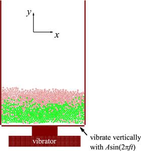
The MD simulations are carried out in a 2D system. Totally one thousand and two hundred spheres (circles), six hundred for each kind of material in general, are placed in a container with gravity field as shown in figure 1. The width of the container is 50 times the size of the sphere diameter d₀=2.0 mm, which results in the spheres piling up about 24 layers. The height of the container is set to be so high that almost no spheres can reach the top of the container except at the beginning of the vibration. The bottom of the container moves vertically with a harmonic displacement function $A\sin (2\pi {ft})$, where A and f are the amplitude and frequency of the vibration, respectively. As in general, frequency f and a dimensionless acceleration amplitude ${\rm{\Gamma }}=4{\pi }^{2}{{Af}}^{2}{g}^{-1}$ are used as control parameters, where $g=9.8\,{\rm{m}}\,{{\rm{s}}}^{-2}$ is the acceleration due to gravity. The other walls of the container are fixed during the vibration.

Figure 1.

New window|Download| PPT slide
Figure 1.The model used in simulation. Two kinds of particles, represented by the open and closed circles for the lighter and heavier particles, respectively, are placed in a container with gravity field. The container is shaked by a harmonic vibrator.


In order to treat multiple particle interactions, which seem to be the most important factor for this system, we use a soft sphere approach in our MD simulations. The Kuwabara–Kono model is used as normal interactions between particles or between particle and side wall [25, 26](1)$ \begin{eqnarray}{F}_{{ij}}^{n}=-{k}_{n}{\xi }_{{ij}}^{3/2}-{\eta }_{n}{\xi }_{{ij}}^{1/2}{V}_{{ij}}^{n},\end{eqnarray}$and the tangential interactions are taken to the minor component in comparison to the viscous friction and dynamic friction [27, 28](2)$ \begin{eqnarray}{F}_{{ij}}^{t}=\min ({\eta }_{t}{V}_{{ij}}^{t},\mu {F}_{{ij}}^{n}).\end{eqnarray}$In equations (1) and (2) ${\xi }_{{ij}}=\max (0,2{d}_{0}-| {{\boldsymbol{r}}}_{i}-{{\boldsymbol{r}}}_{j}| )$ is the overlap of particle i and j, ${{\boldsymbol{V}}}_{{ij}}={V}_{{ij}}^{n}{{\boldsymbol{e}}}_{n}+{V}_{{ij}}^{t}{{\boldsymbol{e}}}_{t}$ is the relative velocity between particle i and j at contact point, and the superscript (subscript) n and t express the normal and tangential components of a vector, respectively. The detail values of the elastic parameters are ${k}_{n}=5.0\times {10}^{9}\,{\rm{N}}/{{\rm{m}}}^{3/2}$, ${\eta }_{n}=300.0\,\mathrm{Ns}/{{\rm{m}}}^{3/2}$, and ${\eta }_{t}=0.3\,{\rm{N}}\,{\rm{s}}\,{{\rm{m}}}^{-1}$, and the coefficient of sliding friction is set to μ=0.2. The time step is taken as Δt=2.0×10⁻⁶ s. These parameters work out the normal restitution coefficient ranging from 0.7 to 0.9 as the impact velocity varies from 1000d₀/s to $1{d}_{0}\,/{\rm{s}}$.

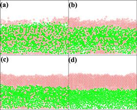
The simulation is carried out under vibration for 40 000 or 60 000 vibration periods from either a completely mixed initial state or a completely separated state. The generation of these initial states will be mentioned below. Figure 2 shows the time evolution of the segregation state during the simulation from a completely mixed initial state, where the acceleration amplitude is set to a relatively high value Γ=24.0 (the amplitude of the vibration A=0.8 mm, about one third of size of the diameter of the particles), and the frequency is set to f=85 Hz. Because the density different is very large, the final segregated state is almost a completely separated state (see figure 2(d)). However, in figures 2(b) and (c), we can see partial segregated states, which have characteristic that the lighter particles tend to go up and form a pure layer on top of the system, while the heavier ones and some of the lighter ones stay at bottom and form a mixed layer. We have called the state as the LMS in the previous work [24]. Figure 2 also shows that the thickness of the pure top layer increases gradually during the simulation, and gives a clear view about how the segregation state changes from a completely mixed state through the LMS state to a completely separated state during the simulation.

Figure 2.

New window|Download| PPT slide
Figure 2.Typical segregated state of a binary granular mixture of the lighter particles with density ${\rho }_{l}=1.0\,{\rm{g}}\,{\mathrm{cm}}^{-3}$ and the heavier ones with density ${\rho }_{h}=20.0\,{\rm{g}}\,{\mathrm{cm}}^{-3}$ from a completely mixed initial state at (a) 30, (b) 100, (c) 300, and (d) 40 000 vibration periods, respectively. The open and closed circles represent the lighter and heavier particles, respectively.


These illustrate that the time evolution of the segregation state can be indicated by the thickness of top layer (if the thickness of whole layer is fixed). In MD simulation, since every particle’s position can be traced during simulations, the average height for each type of particles at certain simulation time can be calculated trivially. The thicknesses of the top layer and the whole layer is calculated by(3)$ \begin{eqnarray}{h}_{l}=\displaystyle \frac{2{N}_{l}({y}_{l}-{y}_{h})}{{N}_{l}+{N}_{h}},\end{eqnarray}$and(4)$ \begin{eqnarray}h=\displaystyle \frac{2({N}_{l}{y}_{l}+{N}_{h}{y}_{h})}{{N}_{l}+{N}_{h}},\end{eqnarray}$where y_h (y_l) and N_h (N_l) are average height and number of the heavier (lighter) particles, respectively.

For equally mixed cases. we have suggested to use twice the ratio of the thickness of the top layer to that of the whole system as an order parameter [24], i.e. $2{h}_{1}/h$. This order parameter can quantitatively describe the degree of particle separation, it is zero when the particles are completely mixed, and is one when the particles are completely separated, and is a number between zero and one when the particles are partially separated. Of course, the order parameter varies with time within a certain range, to obtain an accurate result, we average the data for each thousand vibration periods.

3. Dynamic properties of the segregation

The time evolution of the order parameter $2{h}_{1}/h$ for a system with larger density difference between the lighter and heavier particles (${\rho }_{l}=1.0\,{\rm{g}}\,{\mathrm{cm}}^{-3}$ and ${\rho }_{h}=20.0\,{\rm{g}}\,{\mathrm{cm}}^{-3}$) at a series of vibration amplitude is plotted in figure 3. The simulations are started from both a completely mixed initial state (open symbols) and a pure separated initial state (closed symbols).

Figure 3.

New window|Download| PPT slide
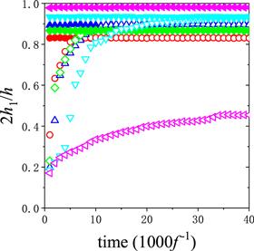
Figure 3.Time evolution of the order parameter for larger density difference between the lighter (${\rho }_{l}=1.0\,{\rm{g}}\,{\mathrm{cm}}^{-3}$) and heavier (${\rho }_{h}=20.0\,{\rm{g}}\,{\mathrm{cm}}^{-3}$) particles at a series of fixed vibration amplitude. The circles, diamonds, upward-pointing triangles, downward-pointing triangles and leftward-pointing triangles are for Γ=19.2, 16.0, 12.8, 8.0 and 4.8, respectively. The open and closed symbols are for the simulations started from a completely mixed initial state and a pure separated initial state, respectively.


The completely mixed initial state is generated by restoring the final state of a simulation for the system without density difference (both ρ_l and ${\rho }_{h}=1.0\,{\rm{g}}\,{\mathrm{cm}}^{-3}$), and the pure segregated initial state is generated by restoring the final state of a simulation for a system with very large density difference between the lighter and heavier particles (${\rho }_{l}=1.0\,{\rm{g}}\,{\mathrm{cm}}^{-3}$ and ${\rho }_{h}=20.0\,{\rm{g}}\,{\mathrm{cm}}^{-3}$).

From figure 3, we can see that the results from two different initial states tend to a same value and keep in that value steadily afterward if the vibration amplitude is not too small. Figure 3 also shows that the speed of the convergence depends seriously on the vibration amplitude. The smaller the vibration amplitude, the slower the convergence will be. When the vibration amplitude is too small (for example Γ=4.8), the simulation from two different initial states does not tend to a same state even at the end of the simulation (40 000 vibration periods).

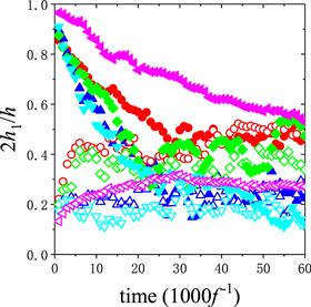
The convergence of the simulation also depends on the density difference between the lighter and heavier particles. Figure 4 depicts the time evolution of the order parameter for a system with smaller density difference at a series of vibration amplitude. Comparing with figure 3, we find that the convergence to the steady state becomes slower in figure 4 for the corresponding vibration amplitude. Another characteristic of the order parameter for the system with smaller density difference is that it fluctuates strongly even after the steady state is reached.

Figure 4.

New window|Download| PPT slide
Figure 4.Time evolution of the order parameter for smaller density difference between the lighter (${\rho }_{l}=1.0\,{\rm{g}}\,{\mathrm{cm}}^{-3}$) and heavier (${\rho }_{h}=3.0\,{\rm{g}}\,{\mathrm{cm}}^{-3}$) particles at a series of vibration amplitude. The symbols are used in the same way as that in figure 3.


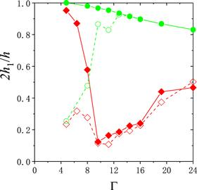
Figure 5 depicts the steady state order parameter as a function of vibration amplitude. The data in this figure is obtained by averaging the order parameters over time for the final 20 000 vibration periods. The total simulation time for ${\rho }_{h}=20.0\,{\rm{g}}\,{\mathrm{cm}}^{-3}$ and $3.0\,{\rm{g}}\,{\mathrm{cm}}^{-3}$ are 40 000 and 60 000 vibration periods, respectively (${\rho }_{l}=1.0\,{\rm{g}}\,{\mathrm{cm}}^{-3}$ for both cases). In figure 5, the order parameters obtained from the completely mixed initial state and the pure separated initial states are almost consistent with each other when the vibration amplitude is larger than Γ=14.0. In this range, the order parameter increases prominently with the vibration amplitude when it is far from its saturated value (see the case of ${\rho }_{l}=1.0\,{\rm{g}}\,{\mathrm{cm}}^{-3}$ and ${\rho }_{h}=3.0\,{\rm{g}}\,{\mathrm{cm}}^{-3}$). However, when the order parameter is near to its saturated value, it decreases slightly with the vibration amplitude (see the case of ${\rho }_{l}=1.0\,{\rm{g}}\,{\mathrm{cm}}^{-3}$ and ${\rho }_{h}=20.0\,{\rm{g}}\,{\mathrm{cm}}^{-3}$). It seems that the order parameter increases originally with the vibration amplitude, but it is also influenced by the non-uniform fluidization during vibration. Because the order parameter is calculated under vibration, the stronger fluidization in the bottom layer may slightly increases the thickness of the mixed layer, and hence decreases the value of the order parameter. Figure 5 shows that this effect becomes stronger as the vibration amplitude increases. This effect is also supported by that the order parameter calculated for the pure segregated state is slightly less than one. The influence of the non-uniform fluidization to the order parameter can be effectively reduced by calculating it from the static segregated state rather than during vibration. However, the order parameter calculated in this way will have larger errors because the average from many segregated state is unpractical. The order parameters obtained from two different initial states split to two branches in small vibration amplitude as shown in figure 5, which means that the simulation does not reach its steady state during the calculations.

Figure 5.

New window|Download| PPT slide
Figure 5.The steady state order parameter as a function of vibration amplitude. The circles are for ${\rho }_{l}=1.0\,{\rm{g}}\,{\mathrm{cm}}^{-3}$ and ${\rho }_{h}=20.0\,{\rm{g}}\,{\mathrm{cm}}^{-3}$, while the diamonds are for ${\rho }_{l}=1.0\,{\rm{g}}\,{\mathrm{cm}}^{-3}$ and ${\rho }_{h}=3.0\,{\rm{g}}\,{\mathrm{cm}}^{-3}$. The open and closed symbols are for the results obtained from a completely mixed initial state and a pure separated initial state, respectively.


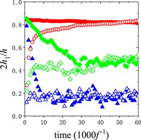
To show the convergent properties of the order parameter for more density combinations, we plot the time evolution of the order parameter for three typical cases at Γ=24.0 in figure 6, in which the simulation has reached its steady state for the final 20 000 vibration periods in all the cases. The figure shows that the steady value of the order parameter becomes smaller and the fluctuation of the order parameter becomes larger when the density difference between lighter and heavier particles decreases.

Figure 6.

New window|Download| PPT slide
Figure 6.Time evolution of the order parameter for the density of the heavier particles being ${\rho }_{h}=8.0\,{\rm{g}}\,{\mathrm{cm}}^{-3}$ (circles), $3.0\,{\rm{g}}\,{\mathrm{cm}}^{-3}$ (diamonds) and $2.0\,{\rm{g}}\,{\mathrm{cm}}^{-3}$ (triangles), respectively. The density of the lighter particles is fixed at ${\rho }_{l}=1.0\,{\rm{g}}\,{\mathrm{cm}}^{-3}$. The open and closed symbols are for the results obtained from a completely mixed initial state and a pure separated initial state, respectively.


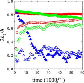
We also found that the convergence to the steady state is slowed down when the total mass in the system increases. Figure 7 presents the time evolution of the order parameter for the heavier combinations of particles, where the density of the lighter particles is fixed at ${\rho }_{l}=2.0\,{\rm{g}}\,{\mathrm{cm}}^{-3}$, and the density ratio between the heavier and lighter particles remain the same as that in figure 6. Figure 7 clearly shows that the simulation hasn’t reached a steady state within the simulation time (60 000 vibration periods), which is long enough for the lighter combinations of particles (see figure 6). We have also checked up this phenomenon by simulating even heavier combinations of particles, such as ρ_l=3.0 and $4.0\,{\rm{g}}\,{\mathrm{cm}}^{-3}$ with fixed density ratio between the heavier and lighter particles, and found that the convergence of the simulation becomes slower as the total mass increases.

Figure 7.

New window|Download| PPT slide
Figure 7.Time evolution of the order parameter for the density of the heavier particles being ${\rho }_{h}=16.0\,{\rm{g}}\,{\mathrm{cm}}^{-3}$ (circles), $6.0\,{\rm{g}}\,{\mathrm{cm}}^{-3}$ (diamonds) and $4.0\,{\rm{g}}\,{\mathrm{cm}}^{-3}$ (triangles), respectively. The density of the lighter particles is fixed at ${\rho }_{l}=2.0\,{\rm{g}}\,{\mathrm{cm}}^{-3}$ in this figure. The open and closed symbols are used in the same way as that in figure 6.

4. Summary and conclusion

In this paper, we have used MD simulations to study a 2D granular mixture made of different densities but of the same size under vertical vibration. We have presented a method that can accurately calculate the order parameter in the simulation. By use of the time evolution of the order parameter, we have discussed some dynamic properties of the segregation, which is almost impossible in the experimental research. We have found that the convergence to the steady state depends at least on the vibration amplitude, the total mass of the particles, and also the density difference between the lighter and heavier particles. The convergence is quicker for larger vibration amplitude, lighter total mass of the particles, and more density difference between the lighter and heavier particles. We have also found that the fluctuation of the order parameter is larger even after the steady state is reached for lighter total mass of the particles and less density difference between the lighter and heavier particles.

Our work has shown that establishing an order parameter is very helpful in the investigation of partial segregation. There are many types of partial segregation. For example, in another experimental study, similar to the system we studied here but where air pressure played an important role, we found another partially segregated state, and its degree of separation can also be described by an order parameter [29]. Our work here can be extended to study the dynamic characteristics of these systems.

Acknowledgments

Project supported by the National Natural Science Foundation of China (Grant Nos. 10875166 and 11274355).

Reference View Option By original order
By published year
By cited within times
By Impact factor

[1]Jaeger H M Nagel S R Behringer R P 1996 Rev. Mod. Phys. 68 1259
DOI:10.1103/RevModPhys.68.1259 [Cited within: 1]

[2]Duran J 1996 Sand, Power, and Grains: An Introduction to the Physics of Granular Materials New York Springer


[3]Kudrolli A 2004 Rep. Prog. Phys. 67 209
DOI:10.1088/0034-4885/67/3/R01 [Cited within: 1]

[4]Williams J C 1976 Powder Technol. 15 245
DOI:10.1016/0032-5910(76)80053-8 [Cited within: 1]

[5]Fan L T Chen Y M Lai F S 1990 Power Technol. 61 255
DOI:10.1016/0032-5910(90)80092-D

[6]Bridgwater J 1976 Power Technol. 15 215
DOI:10.1016/0032-5910(76)80051-4

[7]Xu C Sandali Y Sun G Zheng N Shi Q 2017 Power Technol. 322 92
DOI:10.1016/j.powtec.2017.07.010

[8]Rosato A Strandburg K J Prinz F Swendsen R H 1987 Phys. Rev. Lett. 58 1038
DOI:10.1103/PhysRevLett.58.1038

[9]Jaeger H M Nagel S R 1992 Science 255 1523
DOI:10.1126/science.255.5051.1523 [Cited within: 1]

[10]Jaeger H M Liu C H Nagel S R 1989 Phys. Rev. Lett. 62 40
DOI:10.1103/PhysRevLett.62.40 [Cited within: 1]

[11]Rajchenbach J 1990 Phys. Rev. Lett. 65 2221
DOI:10.1103/PhysRevLett.65.2221

[12]Bretz M Cunningham J B Kurczynski P L Nori F 1992 Phys. Rev. Lett. 69 2431
DOI:10.1103/PhysRevLett.69.2431

[13]Bursik M Patra A Pitman E B Nichita C Macias J L Saucedo R Girina O 2005 Rep. Prog. Phys. 68 271
DOI:10.1088/0034-4885/68/2/R01 [Cited within: 1]

[14]Hong D C Quinn P V Luding S 2001 Phys. Rev. Lett. 86 3423
DOI:10.1103/PhysRevLett.86.3423 [Cited within: 1]

[15]Both J A Hong D C 2002 Phys. Rev. Lett. 88 124301
DOI:10.1103/PhysRevLett.88.124301 [Cited within: 2]

[16]Johanson J R 1978 Chem. Eng. 85 183
DOI:10.1016/0009-8981(78)90238-3 [Cited within: 1]

[17]Hsiau S S Hunt M L 1996 Acta Mech. 114 121
DOI:10.1007/BF01170399 [Cited within: 1]

[18]Hsiau S S Yu H Y 1997 Powder Technol. 93 83
DOI:10.1016/S0032-5910(97)03263-4 [Cited within: 2]

[19]Mobius M E Lauderdale B E Nagel S R Jaeger H M 2001 Nature 414 270
DOI:10.1038/35104697 [Cited within: 1]

[20]Yan X Shi Q Hou M Lu K Chan C K 2003 Phys. Rev. Lett. 91 014302
DOI:10.1103/PhysRevLett.91.014302 [Cited within: 1]

[21]Burtally N King P J Swift M R 2002 Science 295 1877
DOI:10.1126/science.1066850 [Cited within: 2]

[22]Biswas P Sanchez P Swift M R King P J 2003 Phys. Rev. E 68 050301
DOI:10.1103/PhysRevE.68.050301 [Cited within: 2]

[23]Walliser H 2002 Phys. Rev. Lett. 89 189603
DOI:10.1103/PhysRevLett.89.189603 [Cited within: 1]

[24]Shi Q Sun G Hou M Lu K 2007 Phys. Rev. E 75 061302
DOI:10.1103/PhysRevE.75.061302 [Cited within: 3]

[25]Kuwabara G Kono K 1987 Jpn. J. Appl. Phys. 26 1230
DOI:10.1143/JJAP.26.1230 [Cited within: 1]

[26]Schifer J Dippel S Wolf D E 1996 J. Physique I 6 5
DOI:10.1051/jp1:1996129 [Cited within: 1]

[27]Taguchi Y H 1992 J. Physique II 2 2103
DOI:10.1051/jp2:1992255 [Cited within: 1]

[28]Melin S 1994 Phys. Rev. E 49 2353
DOI:10.1103/PhysRevE.49.2353 [Cited within: 1]

[29]Lu C H Shi Q F Yang L Sun G 2008 Chin. Phys. Lett. 25 2542
DOI:10.1088/0256-307X/25/7/058 [Cited within: 1]