Jing Tian^,, Yi-Fan Wang, Hai-Bo QiuSchool of Science, Xi’an University of Posts and Telecommunications, 710121 Xi’an, China

Received:2019-12-23Revised:2020-02-28Accepted:2020-03-2Online:2020-04-22


Abstract
In this paper, by employing an occasionally coupling scheme in a two-species bosonic Josephson junction, it is found that for nonlocal measure synchronized states appearing in the two dynamic modes, known as 0-phase mode and π phase mode, their broken-symmetry can be restored. Nevertheless, there are dramatic differences for the results. For 0-phase mode, we can restore the broken symmetry by turning the nonlocal MS state into a conventional quasiperiodic MS state. However, for the π-phase mode, the broken symmetry is restored accompanied by the appearance of chaotic MS states.
Keywords： symmetry restoring;nonlocal measure synchronization;bosonic Josephson junction


PDF (1051KB)MetadataMetricsRelated articlesExportEndNote|Ris|BibtexFavorite
Cite this article
Jing Tian, Yi-Fan Wang, Hai-Bo Qiu. Symmetry restoring dynamics in a two-species bosonic Josephson junction by using occasional coupling. Communications in Theoretical Physics, 2020, 72(5): 055701- doi:10.1088/1572-9494/ab7ed0

1. Introduction

The creation of Bose–Einstein condensates (BECs) using dilute gases of alkali atoms has provided us with a fantastic platform for study of nonlinear quantum dynamics [1]. Especially, the tunability of nonlinear interactions by employing Feshbach resonances makes it a very attractive candidate for exploring new phenomena involving quantum coherence and nonlinearity [1, 2].

Among many of the specific systems proposed to explore nonlinear quantum dynamics in BECs, the bosonic Josephson junction (BJJ) is especially attractive [3–5]. It has been found that as nonlinear interaction increases in a single species BJJ, it will lead to additional dynamical modes such as macroscopic quantum self-trapping (MQST) or π phase modes [3, 4]. MQST (or π phase mode) phenomenon is characterized by a broken symmetry phase with a population imbalance between the wells. This interaction induced a symmetry-broken phase and has attracted lots of attention over the years [6–11]. For a single species case, the BJJ system has already shown a significantly enriched physical behavior. The physical behavior could be more complicated and interesting by considering multispecies BJJ, i.e., BJJ involving two-species BECs and even more [12, 13]. New physics emerged, including broken symmetry phase in 0-phase modes [14], exchange symmetry breaking [15], and measure synchronization [16], etc.

By concentrating on the physical effects of nonlinear interaction solely in between different species of BECs, it had been found that with increasing the inter-species interaction in a two-species BJJ, a symmetry broken state called nonlocal measure synchronized state (MS) will emerge [16–18]. This novel symmetry broken state exists in both 0-phase and π phase modes. It has been shown that nonlocal MS in 0-phase mode can be achieved through pitchfork bifurcation from a conventional MS state [18]. However, for nonlocal MS in π-phase mode, their appearance are much more complicated due to intrinsic instabilities involved [17].

In this paper, we focus on the nonlocal MS state that have been characterized in a two-species BJJ [16–18]. By applying an occasional coupling scheme, we demonstrate that the broken-symmetry of nonlocal MS can be restored, with the nonlocal MS states turning into conventional MS states, either quasiperodic or chaotic MS states. This paper is organized as follows: first, we describe a two-species bosonic Josephson junction system and the occasional coupling scheme. Second, we present the results by applying occasional coupling scheme for two different kinds of nonlocal MS states that appear in a two-species BJJ. Finally, we summarize the results.

2. A two-species bosonic Josephson junction

The existence of nonlocal measure synchronization has been revealed in a two-species bosonic Josephson junction model system (BJJ) [16–18]. For such a system, possible specific experimental implementations could be an external double-well potential as in [3] or the double-well inside the quantum chip used in [19]. Under the semiclassical theory, the classical Hamiltonian description for this system reads [12],(1)$\begin{eqnarray}\begin{array}{rcl}H & = & {H}_{{\rm{a}}}+{H}_{{\rm{b}}}+{H}_{{\rm{I}}}\\ & = & -\displaystyle \frac{{u}_{{\rm{a}}}}{2}{S}_{{\rm{a}}}^{2}+{\upsilon }_{{\rm{a}}}\sqrt{1-{S}_{{\rm{a}}}^{2}}\cos {\theta }_{{\rm{a}}}\\ & & -\displaystyle \frac{{u}_{{\rm{b}}}}{2}{S}_{{\rm{b}}}^{2}+{\upsilon }_{{\rm{b}}}\sqrt{1-{S}_{{\rm{b}}}^{2}}\cos {\theta }_{{\rm{b}}}-{u}_{\mathrm{ab}}{S}_{{\rm{a}}}{S}_{{\rm{b}},}\end{array}\end{eqnarray}$where a and b represent two different species of BECs. ${H}_{\sigma }=-\tfrac{{u}_{\sigma }}{2}{S}_{\sigma }^{2}+{\upsilon }_{\sigma }\sqrt{1-{S}_{\sigma }^{2}}\cos {\theta }_{\sigma }\quad (\sigma ={\rm{a}},{\rm{b}})$ is the Hamiltonian of a single-specie BJJ [3]. Such that the Hamiltonian equation (1) can be viewed as two coupled single-specie BJJs. The coupling term is ${H}_{{\rm{I}}}=-{u}_{\mathrm{ab}}{S}_{{\rm{a}}}{S}_{{\rm{b}}}$, with u_ab denoting coupling strength.

The corresponding canonical equation of motion can be obtained by computing ${\dot{\theta }}_{\sigma }=\tfrac{\partial H}{\partial {S}_{\sigma }}$ and ${\dot{S}}_{\sigma }=-\tfrac{\partial H}{\partial {\theta }_{\sigma }}$,(2)$\begin{eqnarray}{\dot{\theta }}_{{\rm{a}}}=-{u}_{{\rm{a}}}{S}_{{\rm{a}}}-\displaystyle \frac{{\upsilon }_{{\rm{a}}}{S}_{{\rm{a}}}}{\sqrt{1-{S}_{{\rm{a}}}^{2}}}\cos {\theta }_{{\rm{a}}}-{u}_{\mathrm{ab}}{S}_{{\rm{b}}},\end{eqnarray}$(3)$\begin{eqnarray}{\dot{S}}_{{\rm{a}}}={\upsilon }_{{\rm{a}}}\sqrt{1-{S}_{{\rm{a}}}^{2}}\sin {\theta }_{{\rm{a}}},\end{eqnarray}$(4)$\begin{eqnarray}{\dot{\theta }}_{{\rm{b}}}=-{u}_{{\rm{b}}}{S}_{{\rm{b}}}-\displaystyle \frac{{\upsilon }_{{\rm{b}}}{S}_{{\rm{b}}}}{\sqrt{1-{S}_{{\rm{b}}}^{2}}}\cos {\theta }_{{\rm{b}}}-{u}_{\mathrm{ab}}{S}_{{\rm{a}}},\end{eqnarray}$(5)$\begin{eqnarray}{\dot{S}}_{{\rm{b}}}={\upsilon }_{{\rm{b}}}\sqrt{1-{S}_{{\rm{b}}}^{2}}\sin {\theta }_{{\rm{b}}}.\end{eqnarray}$

The occasional coupling scheme has been proposed to elucidate synchronization in chaotic systems [20–23]. Recently, it has been demonstrated that the occasional coupling scheme not only works for chaos synchronization, but also for measure synchronization [24]. Here by employing the occasional coupling scheme, we derive the equations of motion as follows:(6)$\begin{eqnarray}\dot{X}=f(X)+{u}_{\mathrm{ab}}{\tilde{\lambda }}_{T,\theta }(t)C\cdot g(X).\end{eqnarray}$

Here(7)$\begin{eqnarray}{\tilde{\lambda }}_{T,\theta }(t)=1,\quad {nT}\leqslant t\lt (n+\theta )T,\end{eqnarray}$(8)$\begin{eqnarray}{\tilde{\lambda }}_{T,\theta }(t)=0,\ \ (n+\theta )T\leqslant t\lt (n+1)T,\end{eqnarray}$where T and θ $(\theta \in (0,1])$ are occasional coupling period and the occasional coupling rate. Obviously, when θ=1, it corresponds to the conventional constant coupling scheme. We set the 4-dimensional vector X as $({S}_{{\rm{a}}},{S}_{{\rm{b}}},{\theta }_{{\rm{a}}},{\theta }_{{\rm{b}}})$ for the occasional coupling scheme applied to Hamiltonian equations of a two-species BJJ, whereas f(X), and g(X) equal $({\upsilon }_{{\rm{a}}}\sqrt{1-{S}_{{\rm{a}}}^{2}}\sin {\theta }_{{\rm{a}}},{\upsilon }_{{\rm{b}}}\sqrt{1-{S}_{{\rm{b}}}^{2}}\sin {\theta }_{{\rm{b}}}$, $-{u}_{{\rm{a}}}{S}_{{\rm{a}}}-\tfrac{{\upsilon }_{{\rm{a}}}{S}_{{\rm{a}}}}{\sqrt{1-{S}_{{\rm{a}}}^{2}}}\cos {\theta }_{{\rm{a}}}$, $-{u}_{{\rm{b}}}{S}_{{\rm{b}}}-\tfrac{{\upsilon }_{{\rm{b}}}{S}_{{\rm{b}}}}{\sqrt{1-{S}_{{\rm{b}}}^{2}}}\cos {\theta }_{{\rm{b}}})$, and $(0,0,-{S}_{{\rm{b}}},-{S}_{{\rm{a}}})$. C is a 4×4 matrix, with matrix elements ${C}_{{ij}}={\delta }_{i3}{\delta }_{j3}+{\delta }_{i4}{\delta }_{j4}$ (δ being the Kronecker delta).

The occasional coupling scheme could be implemented by tuning the magnitude of u_ab utilizing the Feshbach resonances [25, 26]. This would allow the interaction strength between two particles to be tuned to essentially any value.

For the two different kinds of nonlocal MS states (0-phase and π phase modes) that appear in a two-species BJJ [16–18], in the following, we shall apply the occasional coupling scheme for both of the nonlocal MS states. To explore the effect of the coupled dynamical behavior by applying occasional coupling to a two-species BJJ system, we use standard fourth-order Runge-kutta method to obtain numerical simulation results.

3. Symmetry restoring versus symmetry breaking

3.1. 0-phase nonlocal MS

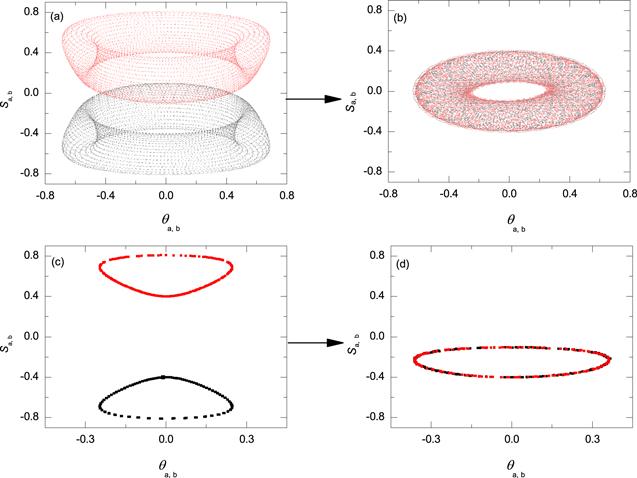
First, we will discuss nonlocal MS in the 0-phase mode, the initial conditions are set as: $({S}_{{\rm{a}}},{\theta }_{{\rm{a}}},{S}_{{\rm{b}}},{\theta }_{{\rm{b}}})=(0.1,0,0.4,0)$, ${u}_{{\rm{a}}}={u}_{{\rm{b}}}=1.2$, ${\upsilon }_{{\rm{a}}}={\upsilon }_{{\rm{b}}}=1.0$.

Figure 1(a) shows the nonlocal MS state in 0-phase mode under conventional constant coupling (without occasional coupling), with two phase space domains for subsystems a and b covering the same acreage, and lying symmetric along S_σ=0 axis. This state, unlike the conventional MS of which the phase space domains cover the identical phase space region, is a manifestation of symmetry breaking underlying measure synchronization.

Figure 1.

New window|Download| PPT slide
Figure 1.Phase space domains and Poincaré section of a two-species BJJ, with u_ab=2.3. Black and red represent the two-species a and b. (a) Phase space domains under constant coupling (without employing occasional coupling). (b) Phase space domains under the occasional coupling scheme (T=0.3, θ=0.4). (c) Poincaré sections under constant coupling (without employing occasional coupling). (b) Poincaré section under occasional coupling, here T=0.3, θ=0.4.


By applying the occasional coupling scheme, the resultant phase space domains are shown in figure 1(b). Here we choose occasional coupling scheme parameters as T=0.3, θ=0.4. Compared with figure 1(a), we note that two phase-space domains completely merge together, covering the phase-space domains with identical invariant measure. This is a characterization for conventional MS state [27].

Furthermore, we have employed Poincaré section analysis to show the essence of the above finding. Figure 1(c) shows the overlapped Poincaré sections without occasional coupling. By solving equations (6) and plotting $({\theta }_{{\rm{a}}},{S}_{{\rm{a}}})$ at each time that θ_b=0 and ${\dot{\theta }}_{{\rm{b}}}\lt 0$. Here the black dots show the Poincaré section slice for subsystem a. We also plot (θ_b, S_b) at each time that ${\theta }_{{\rm{a}}}=0$ and ${\dot{\theta }}_{{\rm{a}}}\gt 0$, the red dots show the Poincaré section slice for subsystem ${\rm{b}}$. We find that the Poincaré section slices for the two subsystems are lying symmetric along S_σ=0, this is a clear indicator for a nonlocal MS state. Figure 1(d) shows the overlapped Poincaré sections obtained after applying the occasional coupling scheme. Here we plot Poincaré section (θ_a, S_a) with θ_b=0 and ${\dot{\theta }}_{{\rm{b}}}\gt 0$ for subsystem a. And we plot Poincaré section $({\theta }_{{\rm{b}}},{S}_{{\rm{b}}})$ with θ_a=0 and ${\dot{\theta }}_{{\rm{a}}}\gt 0$ for subsystem b. It is clearly shown that the two section slices obtained are identical. This indicates a conventional MS state [16]. Apart from this, we observe that the section slice is in a shape of a closed ellipse, which indicates the motion is quasiperiodic. From the above analysis, we reach a conclusion: in 0-phase mode, occasional coupling can restore the broken symmetry of nonlocal MS state, turning it into a conventional quasiperiodic MS state.

In order to explore the above finding in a more systematic way, we calculate averaged energies of each subsystem (a and b) as follows(9)$\begin{eqnarray}\left\langle {E}_{{\rm{a}},{\rm{b}}}\right\rangle =\displaystyle \frac{1}{T}\int {E}_{{\rm{a}},{\rm{b}}}{\rm{d}}t,\end{eqnarray}$with ${E}_{{\rm{a}},{\rm{b}}}=-\tfrac{{u}_{{\rm{a}},{\rm{b}}}}{2}{S}_{{\rm{a}},{\rm{b}}}^{2}+{\upsilon }_{{\rm{a}},{\rm{b}}}\sqrt{1-{S}_{{\rm{a}},{\rm{b}}}^{2}}\cos {\theta }_{{\rm{a}},{\rm{b}}}$ as energy for subsystems a and b.

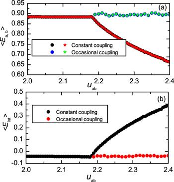
In figure 2(a), we present the result of $\left\langle {E}_{{\rm{a}},{\rm{b}}}\right\rangle $ versus coupling strength u_ab. There is a critical transition in the figure that marks the onset of nonlocal MS at u_ab=u_c=2.2 [18]. Applying occasional coupling in the nonlocal MS region for ${u}_{\mathrm{ab}}\gt {u}_{{\rm{c}}}=2.2$ with parameters $T=0.5,\theta =0.5$, we find that the abrupt decrease of averaged energies beyond u_c=2.2 has been smoothed out, this change due to the occasional coupling indicates that the nonlocal MS states has turned into a conventional MS state.

Figure 2.

New window|Download| PPT slide
Figure 2.Averaged energies versus the coupling strength u_ab. (a) The averaged energy $\left\langle {E}_{{\rm{a}},{\rm{b}}}\right\rangle $ versus the coupling strength u_ab. Nonlocal MS occurs at a critical point u_ab=u_c=2.2 under constant coupling. In contrast, by applying occasional coupling, we find that the critical behavior disappears, here T=0.5, θ=0.5. (b) The averaged interaction energy $\left\langle {E}_{\mathrm{int}}\right\rangle $ versus u_ab. Similarly, here we find that the original critical behavior under constant coupling disappears by applying occasional coupling, here T=0.5, θ=0.5.


In a similar spirit, the averaged interaction energy is calculated,(10)$\begin{eqnarray}\left\langle {E}_{\mathrm{int}}\right\rangle =\displaystyle \frac{1}{T}\int {E}_{{\rm{I}}}{\rm{d}}t,\end{eqnarray}$here ${E}_{{\rm{I}}}=-{u}_{\mathrm{ab}}{S}_{{\rm{a}}}{S}_{{\rm{b}}}$ is the interaction energy between the two different species BECs. As shown in figure 2(b), by increasing coupling strength u_ab, we observe a transition which marks the appearance of nonlocal MS states. Again, by applying occasional coupling for nonlocal MS states (u_ab>u_c=2.2), we find that the abrupt increase of averaged interaction energy beyond u_c=2.2 has been smoothed out. From the perspective of energy characteristics, figure 2 shows that nonlocal MS can be turned into conventional MS by employing an occasional coupling scheme.

For a more quantitative discussion, we introduce an order parameter M to judge whether a state is in MS state or not [28]. Firstly, the phase plane of each subsystem is divided into N×N cells, and here we take N=100. Then, we calculate the number of times that the orbits of the two subsystems have evolved over the same time to reach the same cell (i, j), and define them as ${n}_{i,j}$ and ${n}_{i,j}^{{\prime} }(i,j=1,2,3...N)$. Here we use the following formula to calculate M:(11)$\begin{eqnarray}M=\displaystyle \frac{1}{{\sum }_{i,j}^{N}{c}_{i,j}}\sum _{i,j}^{N}{c}_{i,j}\displaystyle \frac{{\left({n}_{i,j}-{n}_{i,j}^{{\prime} }\right)}^{2}}{{\left({n}_{i,j}+{n}_{i,j}^{{\prime} }\right)}^{2}}.\end{eqnarray}$

The coefficient ${c}_{i,j}=0$ corresponds with both trajectories failing to pass through the cell (i, j), otherwise, ${c}_{i,j}=1$. For MS state, the average times of two trajectories appearing in the corresponding cell (i, j) should be equal, such that M=0. And 0<M≤1 represents the system is not in MS state.

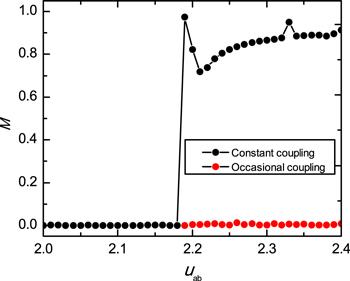
Figure 3 shows the impact of occasional coupling on the system by calculating M. The black dotted line is obtained for the system without occasional coupling. From this part, M is equal to 0 at the beginning, gradually increases the coupling strength u_ab, when u_ab>u_c, the value of M changes within the range of [0,1]. What we need to know is that this part represents the nonlocal MS state. By employing the occasional coupling scheme to this part, and the result is indicated by the red dotted line. After employing the occasional coupling scheme, the value of M decreases to 0, which means that the system turns into the conventional MS.

Figure 3.

New window|Download| PPT slide
Figure 3.Order parameter M versus u_ab. The initial conditions are the same as figure 2. The black dotted line refers to the system under constant coupling, while red indicates the system under the occasional coupling scheme. The value of M clearly indicates that the system becomes a conventional MS after employing the occasional coupling scheme.

3.2. π-phase nonlocal MS

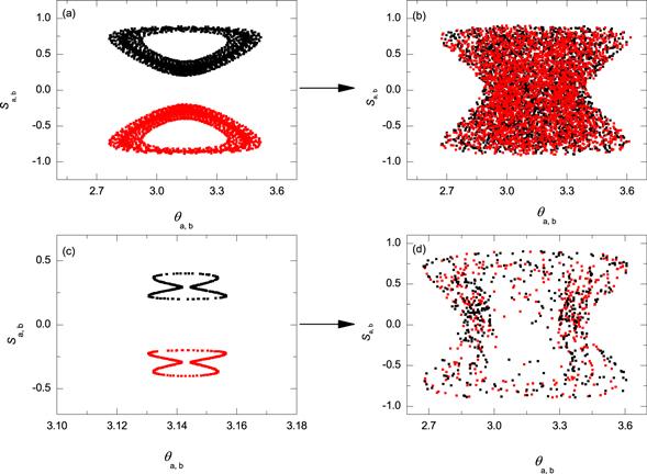
In the following, we discuss the effects of the occasional coupling scheme on nonlocal MS in the π-phase mode. Here, we set the initial condition $({S}_{{\rm{a}}},{\theta }_{{\rm{a}}},{S}_{{\rm{b}}},{\theta }_{{\rm{b}}})=(0.2,\pi ,-0.4,\pi )$, u_a=u_b=1.2, &ugr;_a=&ugr;_b=1.0.

Figures 4(a) and (c) show the phase space domains and Poincaré sections of a two-species BJJ system at u_ab= −0.1622 under constant coupling (without occasional coupling). Figure 4(a) shows a nonlocal MS state, with two phase-space domains of the same acreage lying symmetry along axis ${S}_{{\rm{a}},{\rm{b}}}=0$. Figure 4(c) shows the overlapped Poincaré sections in phase plane (θ_a, S_a) and (θ_b, S_b). The Poincaré section is taken with θ_b=3.14 (θ_a=3.14), ${\dot{\theta }}_{{\rm{b}}}\gt 0$ $({\dot{\theta }}_{{\rm{a}}}\lt 0)$ and presented with red (black) dots. We note that the Poincaré sections in phase plane (θ_a, S_a) and $({\theta }_{{\rm{b}}},{S}_{{\rm{b}}})$ have the same size and lie symmetric along the ${S}_{{\rm{a}},{\rm{b}}}=0$ axis. However, after applying occasional coupling to a two-species BJJ system, the corresponding phase space domains and Poincaré sections are shown in figures 4(b) and (d). Here we set occasional coupling parameters as T=0.3, θ=0.5. As shown in figure 4(b), we find that the two phase space domains merge together, indicating conventional MS is achieved. Figure 4(d) shows the overlapped Poincaré sections under occasional coupling. The Poincaré sections are taken with θ_b= 3.14(θ_a=3.14), ${\dot{\theta }}_{{\rm{b}}}\gt 0({\dot{\theta }}_{{\rm{a}}}\gt 0)$, the resultant section slices are marked with red(black) dots. In figure 4(d), there shows many irregular points for the two subsystems mixed together, indicating that chaotic MS is achieved. To sum up, we find that chaotic MS can be obtained by employing the occasional coupling to nonlocal MS in the π-phase mode.

Figure 4.

New window|Download| PPT slide
Figure 4.Phase space domains and Poincaré section of two-species BJJ, with u_ab=−0.1622. Black and red represent the two-species a and b. (a) phase space domains under constant coupling; (b) phase space domains under occasional coupling, here T=0.3, θ=0.5; (c) Poincaré sections under constant coupling; (d) Poincaré sections under occasional coupling, here T=0.3, θ=0.5.


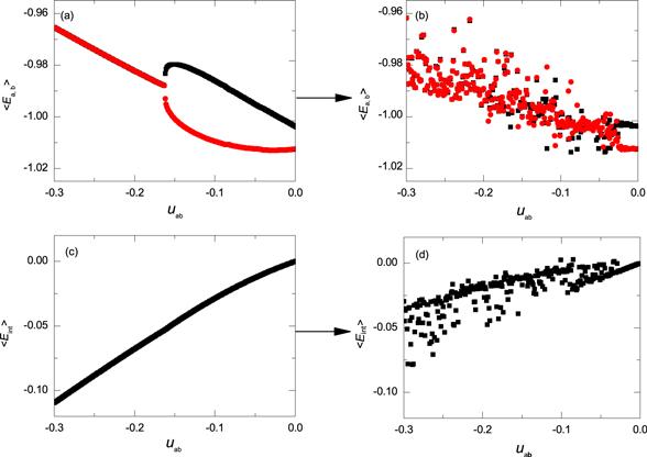
To demonstrate the above finding in a more quantitative way, in figure 5, we show results of the averaged energies ($\left\langle {E}_{{\rm{a}}}\right\rangle $, $\left\langle {E}_{{\rm{b}}}\right\rangle $) and the averaged interaction energy $\left\langle {E}_{\mathrm{int}}\right\rangle $. For the parameters of the occasional coupling, here we choose T=0.5, θ=0.5. Figure 5(a) shows the averaged energies $\left\langle {E}_{{\rm{a}}}\right\rangle $ and $\left\langle {E}_{{\rm{b}}}\right\rangle $ versus the coupling strength u_ab under constant coupling (without occasional coupling). There is a sharp transition at ${u}_{{\rm{c}}}^{{\prime} }=-0.1622$. With ${u}_{\mathrm{ab}}\lt {u}_{{\rm{c}}}^{{\prime} }$, the system turns into nonlocal MS states. It is worth mentioning that, for π-phase mode, it has been found that a two-species BJJ system reaches nonlocal MS without experiencing bifurcations, it is the separatrix crossing that leads the system into nonlocal MS states [16]. In figure 5(b), we show the averaged energies ($\left\langle {E}_{{\rm{a}}}\right\rangle $ and $\left\langle {E}_{{\rm{b}}}\right\rangle $) versus coupling strength under occasional coupling. We note that as u_ab decreases, a large chaotic region emerges where two subsystems have roughly the same energy. This occurs before u_ab reaches ${u}_{{\rm{c}}}^{{\prime} }=-0.1622$. It means that by employing occasional coupling in a region where the system is not in a nonlocal MS state, the system can also be turned into conventional MS states. Figure 5(c) shows the result of the average interaction energy under constant coupling (without occasional coupling), and figure 5(d) shows the result under occasional coupling. It is found that averaged interaction energy becomes larger due to the occasionally coupling. Besides, similar to what has been shown in figure 5(b), we see signs of chaotic motions emerge as u_ab decreases.

Figure 5.

New window|Download| PPT slide
Figure 5.Averaged energies versus the coupling strength u_ab. Black and red dots represent the two-species a and b. (a) The averaged energies of each subsystem under constant coupling; (b) the averaged energies of each subsystem under occasional coupling (T=0.5, θ=0.5); (c) the averaged interaction energy under constant. (d) The averaged interaction energy under occasional coupling (T=0.5, θ=0.5).


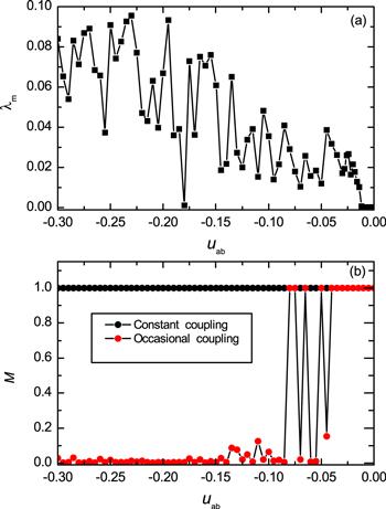
To validate the chaotic MS has been achieved, in the following, we calculate the largest Lyapunov exponent and the order parameter M. In figure 6(a), we show the results of the largest Lyapunov exponent λ_m versus the coupling strength u_ab using occasional coupling, with parameters $T=0.5,\theta =0.5$. Start with u_ab=0, the largest Lyapunov exponent (λ_m=0). It means the system exhibits quasiperiodic motion, as u_ab decreases, chaotic behavior begin to appear, characterized by λ_m>0. The result of the order parameter M versus coupling strength u_ab is presented in figure 6(b). The black and red dotted lines represent the value of M obtained before and after employing occasional coupling respectively. For system not using occasional coupling (under constant coupling), the two phase space domains of the subsystems in π phase mode are always lying symmetric along ${S}_{{\rm{a}},{\rm{b}}}=0$ axis and they are not completely overlapped, so the value of M is in the interval [0, 1]. By decreasing u_ab we find that M reaches 0. This indicates the occurrence of conventional MS.

Figure 6.

New window|Download| PPT slide
Figure 6.(a) The largest Lyapunov exponent λ_m versus u_ab. (b) Order parameter M versus u_ab. The initial conditions are the same as figure 4, with N=100. Red dots (black dots) represent the results for the system with occasional (constant) coupling.

4. Conclusion

In summary, we have shown that by using occasional coupling, the broken symmetry of the nonlocal MS can be restored in a two-species BJJ. We demonstrate this by exploring the phase space domains and Poincaré sections of a two-species BJJ system, revealing that the conventional MS obtained in the 0-phase mode is quasiperiodic MS, while for π-phase mode, it is chaotic MS. Furthermore, we introduce M, which served as order parameter for MS, and shows that by employing occasional coupling to nonlocal MS for both 0-phase mode and π phase mode, M becomes 0. This indicates the occurrence of conventional MS, either for chaotic or quasiperiodic MS.

Acknowledgments

This work was supported by the National Natural Science Foundation of China (Grant No. 11 791 240 559, No. 11 611 540 330, No. 11 402 199), the Natural Science Foundation of Shaanxi Province (Grant No. 2018JM1050, No. 2014JQ1022), and the Education Department Foundation of Shaanxi Province (Grant No. 14JK1676).

Reference View Option By original order
By published year
By cited within times
By Impact factor

[1]Kevrekidis P G Frantzeskakis D J Carretero-Gonzalez R 2008 Emergent Nonlinear Phenomena in Bose–Einstein Condensates Berlin Springer
[Cited within: 2]

[2]Malomed B A 2013 Spontaneous Symmetry Breaking, Self-Trapping, and Josephson Oscillations Berlin Springer
[Cited within: 1]

[3]Albiez M Gati R Folling J Hunsmann S Cristiani M Oberthaler M K 2005 Phys. Rev. Lett. 95 010402
DOI:10.1103/PhysRevLett.95.010402 [Cited within: 4]

[4]Smerzi A Fantoni S Giovanazzi S Shenoy S R 1997 Phys. Rev. Lett. 79 4950
DOI:10.1103/PhysRevLett.79.4950 [Cited within: 1]

[5]Gati R Oberthaler M K 2007 J. Phys. B 40 R61
DOI:10.1088/0953-4075/40/10/R01 [Cited within: 1]

[6]Xiong B Gong J B Pu H Bao W Z Li B W 2009 Phys. Rev. A 79 013626
DOI:10.1103/PhysRevA.79.013626 [Cited within: 1]

[7]Julia-Diaz B Zibold T Oberthaler M K Mele-Messeguer M Martorell J Polls A 2012 Phys. Rev. A 86 023615
DOI:10.1103/PhysRevA.86.023615

[8]Julia-Diaz B Dagnino D Lewenstein M Martorell J Polls A 2010 Phys. Rev. A 81 023615
DOI:10.1103/PhysRevA.81.023615

[9]Tian J Qiu H B 2013 Commun. Theor. Phys. 60 171 174
DOI:10.1088/0253-6102/60/2/05

[10]Zegadlo K B Dror N Trippenbach M Karpierz M A Malomed B A 2016 Phys. Rev. A 93 023644
DOI:10.1103/PhysRevA.93.023644

[11]Spagnolli G et al. 2017 Phys. Rev. Lett. 118 230403
DOI:10.1103/PhysRevLett.118.230403 [Cited within: 1]

[12]Ashhab S Lobo C 2002 Phys. Rev. A 66 013609
DOI:10.1103/PhysRevA.66.013609 [Cited within: 2]

[13]Julia-Diaz B Guilleumas M Lewenstein M Polls A Sanpera A 2009 Phys. Rev. A 80 023616
DOI:10.1103/PhysRevA.80.023616 [Cited within: 1]

[14]Satija I Balakrishnan R Naudus P Heward J Edwards M Clark C W 2009 Phys. Rev. A 79 033616
DOI:10.1103/PhysRevA.79.033616 [Cited within: 1]

[15]Tichy M C Sherson J F Mølmer K 2012 Phys. Rev. A 86 063630
DOI:10.1103/PhysRevA.86.063630 [Cited within: 1]

[16]Tian J Qiu H B Wang G F Chen Y Fu L B 2013 Phys. Rev. E 88 032906
DOI:10.1103/PhysRevE.88.032906 [Cited within: 7]

[17]Tian J Liu J Qiu H B Xi X Q 2017 Front. Phys. 12 120509
DOI:10.1007/s11467-017-0687-5 [Cited within: 1]

[18]Tian J Qiu H B Chen Y 2010 Chin. Phys. Lett. 27 070501
DOI:10.1088/0256-307X/27/7/070501 [Cited within: 6]

[19]Berrada T van Frank S Bücker R Schumm T Schaff J F Schmiedmayer J 2013 Nat. Commun. 4 2077
DOI:10.1038/ncomms3077 [Cited within: 1]

[20]Morgul O Feki M 1997 Phys. Rev. E 55 5004
DOI:10.1103/PhysRevE.55.5004 [Cited within: 1]

[21]Zochowski M 2000 Physica D 145 181 190
DOI:10.1016/S0167-2789(00)00112-3

[22]Chen L Qiu C Huang H B 2009 Phys. Rev. E 79 045101
DOI:10.1103/PhysRevE.79.045101

[23]Li S S Sun N Chen L Wang X G 2018 Phys. Rev. E 98 012304
DOI:10.1103/PhysRevE.98.012304 [Cited within: 1]

[24]Ghosh A Shah T Chakraborty S 2018 Chaos 28 123113
DOI:10.1063/1.5057436 [Cited within: 1]

[25]Papp S B Wieman C E 2006 Phys. Rev. Lett. 97 180404
DOI:10.1103/PhysRevLett.97.180404 [Cited within: 1]

[26]McCarron D J Cho H W Jenkin D L Köppinger M P Cornish S L 2011 Phys. Rev. A 84 011603(R)
DOI:10.1103/PhysRevA.84.011603 [Cited within: 1]

[27]Hampton A Zanette D H 1999 Phys. Rev. Lett. 83 2179
DOI:10.1103/PhysRevLett.83.2179 [Cited within: 1]

[28]Chen S Y Xu H B Wang G R Chen S G 2004 Commun. Theor. Phys. 41 886
DOI:10.1088/0253-6102/41/2/219 [Cited within: 1]