Ya-Hong Hu¹, Zheng-Yi Ma^,21 Institute of Nonlinear Analysis and Department of Mathematics, Lishui University, Lishui 323000, China
2 Department of Mathematics, Zhejiang Sci-Tech University, Hangzhou 310018, China

Corresponding authors: ^?E-mail:ma-zhengyi@163.com

Received:2018-11-25Online:2019-05-1

Fund supported:

fund：Supported by the National Natural Science Foundation of China under Grant Nos.11705077 and 11775104.

Abstract
Starting from the truncated Painlevé expansion, the residual symmetry of the Alice-Bob modified Korteweg-de Vries (AB-mKdV) equation is derived.The residual symmetry is localized and the AB-mKdV equation is transformed into an enlarged system by introducing one new variable.Based on Lie's first theorem, the finite transformation is obtained from the localized residual symmetry.Further, considering the linear superposition of multiple residual symmetries gives rises to N-th B?cklund transformation in the form of the determinant.Moreover, the $P_s T_d$ (the shifted parity and delayed time reversal) symmetric exact solutions (including invariant solution, breaking solution and breaking interaction solution) of AB-mKdV equation are presented and two classes of interaction solutions are depicted by using the particular functions with numerical simulation.
Keywords： Alice-Bob modified Korteweg-de Vries equation;residual symmetry;B?cklund transformation;$P_s T_d$ symmetry;explicit solution


PDF (1043KB)MetadataMetricsRelated articlesExportEndNote|Ris|BibtexFavorite
Cite this article
Ya-Hong Hu, Zheng-Yi Ma. Residual Symmetry of the Alice-Bob Modified Korteweg-de Vries Equation. [J], 2019, 71(5): 489-495 doi:10.1088/0253-6102/71/5/489

1 Introduction

Symmetry has been generalized to the invariance --- that is, the lack of change-under any kind of transformation, for example arbitrary coordinate transformations.^[1] In fact, the classical Lie group method of infinitesimal transformation, the nonclassical Lie group method, and the Clarkson and Kruskal (CK) direct method are viewed as three kinds of powerful tools to find the symmetry structures of integrable nonlinear partial differential equations (NPDEs).^[2-6] Recent results of studying nonlocal symmetries which are derived from the Darboux transformation or the B?cklund transformation, give several different classes of explicit solution, such as the rational one, the Bessel function one, soliton-cnoidal wave interaction one.^[7-11] By introducing suitable prolonged systems, nonlocal symmetries could be localized to local Lie point symmetries and the related finite transformations were considered.^[12-20] Moreover, these facts imply that this kind of approach can generate not only the nonlocal symmetry but also the Lie point symmetry for a given differential system.

In order to explain two-place interrelated physical problems, some Alice-Bob (AB) systems were introduced through the AB-BA principle and $P_s$-$T_d$-$C$ principle with $P_s$ (shifted parity), $T_d$ (delayed time reversal) and $C$ (charge conjugation).^[21] Up to now, the following work has been achieved: a nonlocal AB-KdV system obtained from the coupled KdV equation which describes two area event.^[22] For this nonlocal system, exact solutions including $P_sT_d$ symmetric invariant and breaking ones were derived using the different methods.The multi-soliton solution with a new compact form for the local KdV equation and the nonlocal AB-KdV system was constructed.^[23-24] In particular, a nonlcoal AB-KdV system can reduce from the nonlinear inviscid dissipative and barotropic vorticity equation which can interpret the snow disaster in the winter of 2007/2008 happened in Southern China.Nonlocal integrable peakon equations were also constructed and shown to have peakon solutions.^[25] The $N$-th Darboux transformation of the integrable AB-mKdV system was established.With the help of this kind of Darboux transformation, some $P_sT_d$ symmetric breaking solutions including one- and two-soliton, and rogue wave were presented.^[26]

This paper is organized as follows.In Sec.2, the residual symmetry of the AB-mKdV system is obtained and localized by using the truncated Painlevé expansion method.The finite symmetry transformation is presented by solving the initial value problem.Furthermore, the multiple residual symmetries lead to the $N$-th B?cklund transformation.In Sec.3,the $P_s T_d$ symmetric exact solutions including invariant solution, breaking solution, and breaking interaction one are provided. This summary is given in the last section.

2 Residual Symmetry and B?cklund Trans- formation of the AB-mKdV Equation

The two-place AB-mKdV equation can be described as

(1)$$ A_t + A_{xxx} +6A B A_x=0\, , \quad A=A(x,t), \\ B={P}_s {T}_d A=A(-x+x_0,-t+ t_0), $$
where $x_0$ and $t_0$ are arbitrary constants.^[21]

In fact, the third order Ablowitz-Kaup-Newell-Segur (AKNS) system

(2)$$ u_t + u_{xxx} +6uvu_x=0, \quad v_t +v_{xxx} +6uvv_x=0, $$
has a natural reduction

(3)$$ u_t+u_{xxx}+6u^{2}u_x=0, $$
if $v=u$, which is nothing but the celebrated mKdV equation

(where $u\equiv u(x,t)$, $v\equiv v(x,t))$.

The coupled equation (2) will be reduced to the nonlocal equation

(4)$$ u_t + u_{xxx} +6u[u(-x,-t)]u_x= 0, $$
if $v$ is replaced by $u(-x,-t)$,

which is a special case of the AB-mKdV equation (1) with $x_0 = t_0 = 0.$ It implies that seeking for the exact solution of the AB-mKdV equation (1) transforms to finding the solution of the AKNS system (2). In other words, the solution of the AKNS system (2) may be reduced to those of the AB-mKdV equation (1) by using $v = u(-x,-t)$ due to the $P_sT_d$ symmetric invariance of the AB-mKdV equation (1).

From the leading term analysis of the coupled system (2), the truncated Painlevé expansion

is

(5)$$ u=u_0+\frac{u_1}{f},\quad v=v_0+\frac{v_1}{f}, $$
where the function $f$ is an arbitrary function, and $u_0$, $u_1$, $v_0$, $v_1$ are four functions related to $f$ and its derivatives. Substituting Eq.(5) into Eq.(2) and equating the coefficients of each power of function $f$, we get

(6)$$ u_0=m-\frac{1}{2}\frac{f_{xx}}{f_x} ,\quad u_1=f_x, \\ v_0=m+\frac{1}{2}\frac{f_{xx}}{f_x},\quad v_1=-f_x, $$
with the consistent condition

(7)$$ f_t=-f_{xxx}+\frac{3}{2} \frac{f_{xx}^2}{f_x}-6m^2f_x, $$
where $m$ is an arbitrary constant. Equation~(7) is a typical Schwarzian form of the KdV equation,which is invariant under the M?bious transformation

(8)$$ f\rightarrow\frac{a+bf}{c+df},\quad (ad-bc\neq0). $$
Now, we have the following theorem

Theorem 1 If $f$ is a solution of the Schwarzian equation (7), then

(9)$$ u=m-\frac{1}{2} \frac{f_{xx}}{f_x}+\frac{f_x}{f},\quad v=m+\frac{1}{2} \frac{f_{xx}}{f_x}-\frac{f_x}{f} $$
is a set of solution of the AKNS system (2).

If $f$ is a solution of Eq.(7) and $f(-x,-t)=f(x,t)$, or $f(-x,-t)=-f(x,t)$, then

(10)$$ A=m\mp\frac{1}{2} \frac{f_{xx}}{f_x}\pm\frac{f_x}{f} $$
is a $P_sT_d$ symmetric solution of the AB-mKdV equation (1).

Following the above residual symmetry theorem, one has the residual

(11)$$ u_1=f_x,\quad v_1=-f_x, $$
which corresponds to the nonlocal symmetry of the solution $\{u_0, v_0\}$.^[22]

For the localization of the nonlocal symmetry, we introduce an auxiliary variable $g \equiv g(x,t)=f_x$.

Then, an enlarged system of Eq.(2) is given by

(12)$$ u_t + u_{xxx} +6uvu_x= 0\,, \quad v_t +v_{xxx} +6uvv_x= 0\,, f_t+f_{xxx}- \frac{3}{2} \frac{f_{xx}^2}{f_x}+6m^2f_x=0\,, u=m-\frac{1}{2}\frac{f_{xx}}{f_x}\,,\quad v=m+\frac{1}{2}\frac{f_{xx}}{f_x}\,,\quad g=f_x\,.$$
The corresponding symmetry is

(13)$$ \sigma^u_t+\sigma^u_{xxx}+6uv\sigma^u_x+6uu_x\sigma^v+6vu_x\sigma^u=0, \\ \sigma^v_t+\sigma^v_{xxx}+6uv\sigma^v_x+6vv_x\sigma^u+6uv_x\sigma^v=0, \\ \sigma^f_t+\sigma^f_{xxx}-3 \Big(\frac{f_{xx}}{f_x}\Big)\sigma^f_{xx} +\Big(\frac{f_t}{f_x}+\frac{f_{xxx}}{f_x}+12m^2\Big)\sigma^f_x=0, \\ \sigma^u+\frac{1}{2f_x} \sigma^f_{xx}-\frac{f_{xx}}{2f_x^2}\sigma^f_x=0, \\ \sigma^v-\frac{1}{2f_x} \sigma^f_{xx}+\frac{f_{xx}}{2f_x^2}\sigma^f_x=0, \quad \sigma^g-\sigma^f_x=0. $$
Thus, the derived residual symmetry

$$\{\sigma^u,\sigma^v\} = \{f_x, -f_x\}$$

has the local form

(14)$$ \sigma^u=g,\ \ \sigma^v=-g,\ \ \sigma^f =-f^2,\ \ \sigma^g =-2fg. $$
Furthermore, solving its initial value problem

(15)$$ \frac{d U(\epsilon)}{d \epsilon }=G(\epsilon)\,,\quad \frac{d V(\epsilon)}{d \epsilon }=-G(\epsilon)\,, \frac{d F(\epsilon)}{d \epsilon }=-F(\epsilon)^2\,,\quad \frac{d G(\epsilon)}{d \epsilon }=-2F(\epsilon)G(\epsilon)\,, U(0) = u\,,\quad V(0) = v\,,\quad $$
with $\epsilon$ being an arbitrary group parameter, leads to the finite transformation theorem.

Theorem 2 (B?cklund transformation theorem of the coupled system (2)) If $\{ u, v, f, g \}$ is a solution of Eqs.(12), so is $\{ U(\epsilon),V(\epsilon),F(\epsilon),G(\epsilon) \}$ for Eq.(15), where

(16)$$ \ U(\epsilon) = u+\frac{\epsilon g}{1+\epsilon f}\,,\quad V(\epsilon) = v-\frac{\epsilon g}{1+\epsilon f}\,, \\ \ F(\epsilon) = \frac{f}{1+\epsilon f}\,,\quad G(\epsilon) = \frac{ g}{(1+\epsilon f)^2}\,.$$
Based on Theorem 2, we consider the B?cklund transformation for the AB-mKdV equation (1). It immediately reaches the B?cklund transformation theorem for Eq.(1) from the coupled system (2).

Theorem 3 (B?cklund transformation theorem of the AB-mKdV equation (1))

If A is a solution of the AB-mKdV equation (1), $f$ is a solution of Eq.(7) and satisfies $f(-x,-t)=f(x,t)$, then

(17)$$ A^{'}(\epsilon) = A\pm[\ln(1+\epsilon f)]_x, $$
is a $P_sT_d$ symmetry breaking solution of Eq.(1).

For example, the composite function $f$

(18)$$ f= C_0+C_1\int^{(x-6m^2t)t^{-1/3}}\hphantom{f=}\!\times \!{\frac{d X}{(C_2\text{AiryAi}(-({1}/{\sqrt[3]{6}})X)\!+{\rm AiryBi}(-({1}/{\sqrt[3]{6}})X))^2}}$$
is satisfied, where AiryAi, AiryBi-the Airy Ai and Bi wave functions. The Airy wave functions AiryAi and AiryBi are linearly independent solutions for $w$ in the equation $w(x)_{xx}-zw(x)=0$. $C_0$, $C_1$, and $C_2$ are three constants.

Furthermore, since the symmetry equations (13) are all linear and Eq.(7) possesses infinitely

many solutions, one can get the infinitely many residual

symmetries

(19)$$ \sigma_n^u= \sum_{i=1}^n c_if_{i,x},\quad \sigma_n^v= -\sum_{i=1}^n c_if_{i,x}, $$
for arbitrary natural number $n$, where $f_i\; (i = 1,2,\ldots,n)$ are all solutions of Eq.(7), i.e.

(20)$$ f_{i,t}+f_{i,xxx}- \frac{3}{2} \frac{f_{i,xx}^2}{f_{i,x}}+6m^2f_{i,x}=0\,,$$
and $u$ and $v$ obey the relations

(21)$$u=m-\frac{1}{2}\frac{f_{i,xx}}{f_{i,x}}\,, \quad v=m+\frac{1}{2}\frac{f_{i,xx}}{f_{i,x}}\,.$$
For localization of the residual symmetry $\sigma_n^u$ and $\sigma_n^v$, one can introduce following variables $g_i\equiv g_i(x, t)$ given by

(22)$$ g_i=f_{i,x}, $$
for $i = 1,2,\ldots,n$.

The nonlocal symmetry (19) becomes a Lie point symmetry

(23)$$ \sigma_n^u= \sum_{i=1}^n c_ig_i,\quad \sigma_n^v= -\sum_{i=1}^n c_ig_i, \\ \sigma^{f_i}=-c_if_i^2- \sum_{j\neq i}^n c_j f_if_j, \\ \sigma^{g_i}=-2c_if_i g_i- \sum_{j\neq i}^n c_j (f_i g_j+g_i f_j). $$
By solving its initial value problem

(24) $$\frac{d U(\epsilon)}{d \epsilon}=\sum_{i=1}^n c_iG_i(\epsilon)\,,\quad \frac{d V(\epsilon)}{d \epsilon }=-\sum_{i=1}^n c_iG_i(\epsilon)\,, \frac{d F_i(\epsilon)}{d \epsilon }=-c_i F_i(\epsilon)^2- \sum_{j\neq i}^n c_j F_i(\epsilon)F_j(\epsilon)\,, \frac{d G_i(\epsilon)}{d \epsilon }=-2c_i F_i(\epsilon) G_i(\epsilon)\hphantom{\frac{d G_i(\epsilon)}{d \epsilon }=}- \sum_{j\neq i}^n c_j [F_i(\epsilon) G_j(\epsilon)+G_i(\epsilon) F_j(\epsilon)]\,, U(0) = u\,,\ \ V(0) = v\,,\ \ F_i(0) =f_i\,,\ \ G_i(0) = g_i\,,$$
one can arrive at the following $N$-th B?cklund transformation theorem.

Theorem 4 ($N$-th B?cklund transformation theorem of the coupled system (2))

If $\{u, v, f_i , g_i, i = 1,2,\ldots,n\}$ is a solution of the prolonged system (2) and Eqs.(20)--(22), so is

$$ \{U(\epsilon), V(\epsilon),F_i(\epsilon), G_i (\epsilon), i = 1,2,\ldots,n \}, $$

where

(25)$ U(\epsilon)=u+(ln △)_x\,,\quad V(\epsilon)=v-(ln △)_x\,,\\\ \ F_i(\epsilon)=\frac{delta_i}{delta}\,,\quad G_i(\epsilon)=F_{i,x}(\epsilon)\,,$$
with $delta$ and $delta_i$ are determinants of the matrices $M$ and $M_i$ expressed by

$$ \ M=\begin{pmatrix} \epsilon c_1 f_1+1 \ \epsilon c_1\omega_{12} \ \cdot\cdot\cdot \ \epsilon c_1\omega_{1j} \ \cdot\cdot\cdot \ \epsilon c_1\omega_{1n} \\ \epsilon c_2\omega_{12} \ \epsilon c_2 f_2+1 \ \cdot\cdot\cdot \ \epsilon c_2\omega_{2j} \ \cdot\cdot\cdot \ \epsilon c_1\omega_{2n} \\ \vdots \ \vdots \ \vdots \ \vdots \ \vdots \ \vdots \\ \epsilon c_j\omega_{1j} \ \epsilon c_j\omega_{2j} \ \cdot\cdot\cdot \ \epsilon c_j f_j+1 \ \cdot\cdot\cdot\cdot \ \epsilon c_j\omega_{jn} \\ \vdots \ \vdots \ \vdots \ \vdots \ \vdots \ \vdots \\ \epsilon c_n\omega_{1n} \ \epsilon c_n\omega_{2n} \ \cdot\cdot\cdot \ \epsilon c_n\omega_{jn} \ \cdot\cdot\cdot\cdot \ \epsilon c_n f_n+1 \end{pmatrix},\quad \omega_{ij}=\sqrt{f_i f_j}\,, \\ M_i=\begin{pmatrix} \epsilon c_1 f_1+1 \ \epsilon c_1\omega_{12} \ \cdot\cdot\cdot \ \epsilon c_1\omega_{1,i-1} \ \epsilon c_1\omega_{1i} \ \epsilon c_1\omega_{1,i+1} \ \cdot\cdot\cdot \ \epsilon c_1\omega_{1n} \\ \epsilon c_2\omega_{12} \ \epsilon c_2 f_2+1 \ \cdot\cdot\cdot \ \epsilon c_2\omega_{2,i-1} \ \epsilon c_2\omega_{2i} \ \epsilon c_2\omega_{2,i+1} \ \cdot\cdot\cdot \ \epsilon c_1\omega_{2n} \\ \vdots \ \vdots \ \vdots \ \vdots \ \vdots \ \vdots \ \vdots \ \vdots \\ \epsilon c_{i-1}\omega_{1,i-1} \ \epsilon c_{i-1}\omega_{2,i-1} \ \cdot\cdot\cdot \ \epsilon c_{i-1} f_{i-1}+1 \ \epsilon c_{i-1}\omega_{i-1,i} \ \epsilon c_{i-1}\omega_{i-1,i+1} \ \cdot\cdot\cdot\cdot \ \epsilon c_{i-1}\omega_{i-1,n} \\ \omega_{1i} \ \omega_{2i} \ \cdot\cdot\cdot \ \omega_{i-1,i} \ f_i \ \omega_{i,i+1} \ \cdot\cdot\cdot\cdot \ \omega_{in} \\ \epsilon c_{i+1}\omega_{1,i+1} \ \epsilon c_{i+1}\omega_{2,i+1} \ \cdot\cdot\cdot \ \epsilon c_{i+1}\omega_{i-1,i+1} \ \epsilon c_{i+1}\omega_{i,i+1} \ \epsilon c_{i+1} f_{i+1}+1 \ \cdot\cdot\cdot\cdot \ \epsilon c_{i+1}\omega_{i+1,n} \\ \vdots \ \vdots \ \vdots \ \vdots \ \vdots \ \vdots \ \vdots \ \vdots \\ \epsilon c_n\omega_{1n} \ \epsilon c_n\omega_{2n} \ \cdot\cdot\cdot \ \epsilon c_n\omega_{i-1,n} \ \epsilon c_n\omega_{in} \ \epsilon c_n\omega_{i+1,n} \ \cdot\cdot\cdot\cdot \ \epsilon c_n f_n+1 \end{pmatrix},$$

respectively.

Theorem 5 ($N$-th B?cklund transformation theorem of the AB-mKdV equation (1))

If A is solution of the AB-mKdV equation (1), $ f_i\;(i = 1,2,\ldots, n) $ are solutions of Eq.(20) and have the even function property $f_i(-x,-t)=f_i(x,t)$, then

(26)$$ A'(\epsilon) = A\pm(ln \delta)_x, $$
is a $P_sT_d$ symmetric breaking solution of the AB-mKdV equation (1).

3 The $P_s T_d$ Symmetry Exact Solutions of the AB-mKdV Equation

Recently, it is found that several AB systems have exact solutions of the $P_sT_d$ symmetry invariant or the $P_sT_d$ symmetry breaking.^{[21-22,24-26]} Through the trial function method, the AB-mKdV system (1) has solutions of the following properties.

Case 1 The $P_s T_d$ symmetry invariant solutions

(27) $$ A_1=delta k\text{sech}\Big[k\Big(x-\frac{x_0}{2}\Big)-k^3\Big(t-\frac{t_0}{2}\Big)\Big], $$
(28) $$A_2=delta nk\text{cn}\Big[k\Big(x-\frac{x_0}{2}\Big)+k^3(1-2n^2)\Big(t-\frac{t_0}{2}\Big),n\Big],$$
(29) $$ A_3=delta k\text{dn}\Big[k\Big(x-\frac{x_0}{2}\Big)+k^3(1-2n^2)\Big(t-\frac{t_0}{2}\Big),n\Big],$$
where $k$, $x_0$, $t_0$ are arbitrary constants and $delta^2=1$.

Case 2 The $P_s T_d$ symmetry breaking solutions

(30)$$ A_4=\;a_0+delta k \tanh\Big[k\Big(x-\frac{x_0}{2}\Big) +2k(k^2-3a_0^2)\Big(t-\frac{t_0}{2}\Big)\Big]\,,$$
(31)$$ A_5=\;a_0+delta k \text{coth}\Big[k\Big(x-\frac{x_0}{2}\Big)+2k(k^2-3a_0^2)\Big(t-\frac{t_0}{2}\Big)\Big]\,,$$
(32)$$ A_6=\;a_0+delta nk\text{sn}\Big[k\Big(x-\frac{x_0}{2}\Big) \ +k((m^2+1)k^2-6a_0^2)\Big(t-\frac{t_0}{2}\Big),n\Big]\,.$$
Case 3 The $P_s T_d$ symmetry breaking interaction solutions

After setting

(33)$$ f=\frac{1}{1-\tanh(\omega)}, $$
with $\omega\equiv\omega(x,t)$, and substituting Eq.(33) into Eqs.(5)--(7), we get one solution of the coupled system (2) is

(34)$$ \ u=m-\frac{1}{2}\frac{\omega_{xx}}{\omega_x}+\omega_x \tanh(\omega)\,, \\ \ \ v=m+\frac{1}{2}\frac{\omega_{xx}}{\omega_x}-\omega_x \tanh(\omega)\,,$$
with the associated compatibility condition

(35)$$ \omega_t=-\omega_{xxx}+\frac{3}{2}\frac{\omega_{xx}^2}{\omega_x}+2\omega_x^3-6m^2\omega_x . $$
For the $P_s T_d$ symmetry breaking interaction solution between a soliton and a cnoidal wave, one can take the ansatz of Eq.(35)

(36)$$ \omega =\frac{x-V_1t}{delta_1}+c_1\text{arctanh} \Big[c_2\text{sn}\Big(\frac{x-V_2t}{delta_2},n\Big)\Big]. $$
Substituting the ansatz (36) into Eq.(35) and vanishing the coefficients of the different powers of Jacobi elliptic function, two sets of nontrivial solution $V_1$, $V_2$, $c_1$, $c_2$, $delta_2$ can be determined as

(37) $$ V_1 = \frac{2(3m^2delta_1^2-3n^2-1)}{delta_1^2}\,, V_2 =\frac{2(3m^2delta_1^2+n^2-5)}{delta_1^2}\,, c_1 =\frac{1}{2}delta\,,\quad c_2 = n\,,\quad delta_2 = \frac{1}{2}delta_1\,,\quad delta^2=1\,, $$
(38) $$ V_1 = \frac{2[3(n+1)^2m^2delta_1^2-n^2-14n-1]}{delta_1^2(n+1)^2}\,, V_2=\frac{2[3(n+1)^2m^2delta_1^2-5n^2-6n-5]}{delta_1^2(n+1)^2}\,, c_1 =delta \,,\quad c_2 = \sqrt{n}\,,\quad delta_2 = \frac{1}{2}(n+1)delta_1\,,\quad delta^2=1\,,$$
where $delta_1$ is an arbitrary constant.

Substituting Eq.(36) into Eq.(34), one soliton-cnoidal wave interaction solution of Eq.(2) is

(39) $$ u=m+\frac{c_1c_2S[(c_2^2+n^2c_2^2-2n^2)S^2+1-2c_2^2+n^2]delta_1}{2delta_2(1-c_2^2S^2)(delta_2-delta_2c_2^2S^2+c_1c_2CDdelta_1)}+\Big(\frac{1}{delta_1}+\frac{c_2c_1CD}{delta_2(1-c_2^2S^2)}\Big) \tanh(\omega)\,, \\ v=m-\frac{c_1c_2S[(c_2^2+n^2c_2^2-2n^2)S^2+1-2c_2^2+n^2]delta_1}{2delta_2(1-c_2^2S^2)(delta_2-delta_2c_2^2S^2+c_1c_2CDdelta_1)}-\Big(\frac{1}{delta_1}+\frac{c_2c_1CD}{delta_2(1-c_2^2S^2)}\Big) \tanh(\omega)\,,$$
with

$$ S=\text{sn}\Big(\frac{x-V_2t}{delta_2}, n\Big),\quad C=\text{cn}\Big(\frac{x-V_2t}{delta_2}, n\Big),\quad D=\text{dn}\Big(\frac{x-V_2t}{delta_2}, n\Big). $$

Therefore, after substituting Eqs.(37) and (38) into Eq.(39), we have the $P_s T_d$ symmetry breaking interaction solutions of Eq.(1)

(40)$$ A_7=m\mp\frac{(n^2-1)ndelta S}{delta_1(1-n^2S^2+delta CD)}\pm\frac{1}{delta_1} \Big(1+delta\frac{ C}{D}\Big)\tanh(\omega), $$
with

(41)$$ \ \omega=\frac{1}{delta_1}\Big[\Big(x-\frac{x_0}{2}\Big)-\frac{3m^2delta_1^2-3n^2-1}{delta_1^2}(2t-t_0)\Big]+\frac{1}{2}delta\arctan(nS)\,,\\\ \ S=\text{sn}(X_1, n)\,, \quad C=\text{cn}(X_1, n)\,,\quad D=\text{dn}(X_1, n)\,,\quad X_1\equiv\frac{2}{delta_1}\Big[\Big(x-\frac{x_0}{2}\Big)-\frac{3m^2delta_1^2+n^2-5}{delta_1^2}(2t-t_0)\Big]\,,\\\ \ A_8=m\pm\frac{2delta(n-1)^2\sqrt{n}S(1+nS^2)}{delta_1(n+1)(1-n S^2)(D+delta \sqrt{n}C)^2}\pm\frac{1}{delta_1}\Big[1+\frac{2delta\sqrt{n}CD}{(n+1)(1-nS^2)}\Big] \tanh(\omega)\,, $$
with

$$ \omega=\frac{1}{delta_1}\Big[\Big(x-\frac{x_0}{2}\Big)-\frac{3(n+1)^2m^2delta_1^2-n^2 -14n-1}{delta_1^2(n+1)^2}(2t-t_0)\Big]+delta\arctan(\sqrt{n}S), \\\ S=\text{sn}(X_2, n), \quad C=\text{cn}(X_2, n),\quad D=\text{dn}(X_2, n), \\\ X_2\equiv\frac{2}{delta_1(n+1)}\Big[\Big(x-\frac{x_0}{2}\Big)-\frac{3(n+1)^2m^2delta_1^2-5n^2-6n-5} {delta_1^2(n+1)^2}(2t- t_0 )\Big]. $$

New window|Download| PPT slide
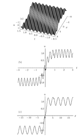
Fig.1(a) The three-dimensional profile of the solution $A_7$ in Eq.(40) at the region x∈ ^{[8, 8]}$, $t\in [-1.5, 1.5]$. (b) The two-dimensional profile with $x=0$. (c) The two-dimensional profile at time $t=0$.



The solution (40) describes the interaction between a kink and periodic waves, which has the potential application in physical setting.

In Fig.1, the interaction behavior between a kink soliton and cnoidal waves given by the solution $A_7$ in Eq.(40) is plotted when the parameters $delta=-1$, $delta_1=1$, $n=0.2$, $m=0$, $x_0=0$, $t_0=0$.

Figure 1(a) displays the profile at x∈ ^{[8, 8]}, $t$$\in$ [-1.5, 1.5]$. One can observe that in this process the kink soliton propagates on the periodic wave background.

Figures~1(b) and 1(c) are profiles with $x=0$ and at time $t=0$, respectively.

New window|Download| PPT slide
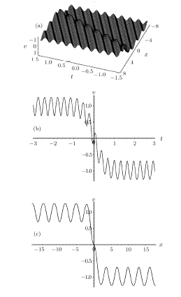
Fig.2(a) The three-dimensional profile of the another solution $A_7$ in Eq.(40) at the region x∈^{[8, 8]}$, $t\in [-1.5, 1.5]$. (b) The two-dimensional profile with $x=0$. (c) The two-dimensional profile at time $t=0$.



Figure 2 depicts a reversal structure of Fig.1 by the another solution $A_7$ (which is $P_sT_d$ symmetry of the first solution $A_7$ for Eq.(1)).This corresponds to the phenomenon that the shifted parity and delayed time reversal are applied to describe two-place events.

New window|Download| PPT slide
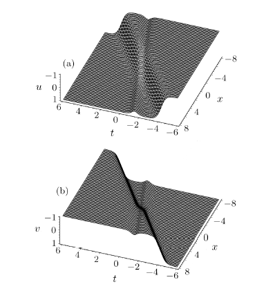
Fig.3(a) The interaction between a soliton and kink given by $A_9$ in Eq.(44) with $delta_1=1$, $m=0$, $c_2=0.5$. (b) The structure of another solution $A_9$ represents a reversal shape of (a).



As a special case, when substituting $n=1$ into Eq.(36), we obtain

(42)$$dis{\omega =\frac{x-V_1t}{delta_1}+c_1\text{arctanh}\Big(c_2\tanh\Big(\frac{x-V_2t}{delta_2}\Big)\Big)\,.}$$
Substituting Eq.(42) into Eq.(35), then

(43)$$ \ delta_2 = \frac{delta_1}{c_2}\,,\quad V_1 = \frac{2(3m^2delta_1^2-1)}{delta_1^2}\,, \\\ \ V_2 = \frac{2(3m^2delta_1^2+2c_2^2-3)}{delta_1^2}\,,\quad c_1=-1\,, $$
where $delta_1$, $c_2$ are two arbitrary constants.

System (1) has the following solution

(44)$$ A_9= \;m\pm\frac{c_2^3T(1-T^2)}{delta_1(1-c_2^2T^2)}\\\\pm \ \;\frac{1-c_2^2}{delta_1(1-c_2^2T^2)}\tanh(\omega)\,, $$
with

$$ \ \omega=\frac{1}{delta_1}\Big[\Big(x-\frac{x_0}{2}\Big)-\frac{3m^2delta_1^2-1}{delta1^2}(2t-t_0)\Big]\\\ \ \hphantom{\omega=}+\text{arctanh}(c_2T)\,,\\\ \ T\!=\!\tanh\Big\{\frac{c_2}{delta_1}\Big[\Big(x-\frac{x_0}{2}\Big)-\!\frac{3m^2delta_1^2+2c_2^2-3}{delta1^2}(2t-t_0)\Big]\Big\}\,.$$

Figure 3 shows the solution $A_9$ of Eq.(44) when taking $delta_1=1$, $m=0$, $c_2=0.5$. From Fig.3(a), one can find that we have a bright soliton and a kink before the interaction.However, after the interaction, the soliton becomes a dark (gray) soliton but the kink is unchanged.The nonlocal interaction in the model results in such type of transition for the solution $A_9$.Figure 3(b) stands for a reversal structure of Fig.3(a) for another solution $A_9$.

4 Summary

In this paper, a special AB-mKdV system is derived from mKdV equation to describe two-place interrelated event.This system is nonlocal and possesses $P_sT_d$ symmetry.Starting from the truncated Painlevé expansion,the residual symmetry is obtained and further localized to Lie point symmetry by extending the AB-mKdV system to an enlarged one.At the same time, the finite transformation is presented.Further, we consider the multiple residual symmetry via the linear superposition and give its finite transformation, which is nothing but the $N$-th B?cklund transformation.It is shown that this type of the B?cklund transformation is given in terms of determinants and can generate new solution from a seed one. Moreover, based on the trial function approach, the $P_s T_d$ symmetric solutions (including invariant solution, breaking solution and breaking interaction solution) of AB-mKdV equation are presented and two classes of interaction solutions are depicted by using the particular functions with numerical simulation.

Reference View Option By original order
By published year
By cited within times
By Impact factor

[1] G. Costa and G. Fogli , Symmetries and Group Theory in Particle Physics: an Introduction to Space-Time and Internal Symmetries, Springer-Verlag, Berlin ( 2012).
[Cited within: 1]

[2] P.A Clarkson . and M. D. Kruskal , J. Math. Phys. 30(1989) 2201.
[Cited within: 1]

[3] P.A Clarkson . and E. L. Mansfield, SIAM J. Appl. Math. 54(1994) 1693.


[4] G. W. Bluman and J. D. Cole , Similarity Methods for Differential Equations, Springer-Verlag Berlin ( 1974).


[5] G.W Bluman . andS. Kumei , it Symmetries and


Differential Equation , Springer-Verlag,Berlin ( 1989).


[6] P. J. Olver , Applications of Lie Groups to Differential Equations, Springer-Verlag,NewYork ( 1993).
[Cited within: 1]

[7] S. Y. Lou, X. R. Hu, Y. Chen, J. Phys . A: Math. Theor. 45(2012) 155209.
[Cited within: 1]

[8] X. R. Hu, S. Y. Lou, Y. Chen , Phys. Rev. E . 85 ( 2012) 056607.
[Cited within: 6]

[9] J. C. Chen, Z. Y. Ma, Y. H. Hu, . J. Math.Anal Appl.460(2018) 987.


[10] J.C Chen . and S. D. Zhu , Appl. Math. Lett. 73(2017) 136.


[11] J.C Chen . and Z. Y .Ma , Appl. Math. Lett. 64(2017) 87.
[Cited within: 1]

[12] Y. Jin, M. Jia, S. Y. Lou , Commun. Theor. Phys. 58(2012) 795.
[Cited within: 1]

[13] X. N. Gao, S. Y. Lou, X. Y. Tang , J. High Energy Phys. 05(2013) 029.


[14] Z. Y. Ma, J. X. Fei, J. C. Chen, Naturforsch . 72(2017) 863.


[15] X. Z. Liu, J. Yu, B. Ren, J. R. Yang , Chin. Phys. B 24 ( 2015) 010203.


[16] L.L Huang and Y. Chen ., Nonlinear Dyn. 92(2018) 221.


[17] Z. Y. Ma, J. X. Fei, J. C. Chen , Commun. Theor. Phys. 70(2018) 31.


[18] J. F. Song, Y. H. Hu, Z. Y. Ma , Nonlinear Dyn. 90(2017) 575.


[19] J.C Chen .and S. D. Zhu , Appl. Math. Lett. 73(2017) 136.


[20] S.D Zhu . andJ. F .Song, Appl. Math. Lett. 83(2018) 33.
[Cited within: 1]

[21] S. Y. Lou , rXiv: 1603. 03975[nlin.SI]( 2016).
[Cited within: 3]

[22] M. Jia and S. Y. Lou , Phys. Lett. A 382 ( 2018) 1157.
[Cited within: 3]

[23] S. Y. Lou , arXiv: 1308. 1140[nlin.SI]( 2013).
[Cited within: 1]

[24] S.Y Lou . and F. Huang , Sci.Rep. 7(2017) 869.
[Cited within: 2]

[25] S.Y Lou .and Z. J .Qiao. Chin .Phys. Lett. 34(2017) 100201.
[Cited within: 1]

[26] C. C. Li, S. Y. Lou, M. Jia , Nonlinear Dyn. 93(2018) 1799.
[Cited within: 2]